Business planning and financial modeling for microfinance insti phần 6 ppsx

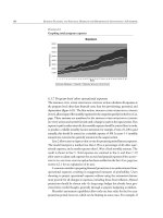
6.3.7 Program-level other operational expenses
The program-level other operational expenses section calculates all expenses at
the program level other than financial costs, loan loss provisioning, personnel, and
depreciation (figure 6.13). The first section, program other operational expenses
[input], allows input of the monthly expenses for the categories specified on the Inst.Cap.
page. These amounts are transferred to the program other operational expenses
[output] section and carried forward until a change is made in the input section. If an
expense is paid at other intervals, the monthly expense should be entered here in order
to produce a reliable monthly income statement; for example, if rent of 1,200 is paid
annually, this should be entered as a monthly expense of 100. In years 3–5 monthly
amounts are converted to quarterly amounts in the output section.
Line 2 allows users to input a value or rate for projecting miscellaneous expenses.
The model interprets a number less than 1.00 as a percentage of all other oper-
ational expenses, and a number greater than 1.00 as a fixed monthly amount. The
result is shown in line 5. Total expenses are summed in line 6, and lines 7–10
allow users to adjust cash expenses for accrued and prepaid expenses if the adjust-
ments to cash flow analysis option has been enabled on the Inst.Cap. page (see
section 6.2.1 for an explanation of its use).
A common mistake in preparing financial projections is to underestimate future
operational expenses, resulting in exaggerated estimates of profitability. Users
choosing to project operational expenses without using the automation feature
must provide for all changes in expenses, including those from inflation. Manual
projections should be chosen only if a long-range budget has already been gen-
erated after careful thought, generally through a separate budgeting worksheet.
Microfin’s automation capabilities allow only one base value for the five-year
projection period, however, which can be limiting in some cases. For example, if
108 BUSINESS PLANNING AND FINANCIAL MODELING FOR MICROFINANCE INSTITUTIONS: A HANDBOOK
FIGURE 6.12
Graphing total program expenses
the number of loan officers is projected to double, will larger branch offices need
to be rented, increasing rental expense per branch? If so, a combination of automa-

tion and manual overrides could be used. For somewhat less precise results,
rental expense could be projected to increase at a rate greater than inflation to
account for increasing costs per branch. Or expenses could be projected to increase
by less than inflation to reflect economies of scale.
Microfin provides a means for automating the projection of other operational
expenses similar to that used for staffing. On the Inst.Cap. page users can link
operational expenses to a percentage of monthly or annual inflation, the number
of loan officers, the number of program staff, the number of borrowers, the num-
ber of depositors, the number of branches, or a combination of these (figure 6.14).
The link to inflation can be used independent of other links; in this case the model
applies the inflation adjustment to whatever amount is entered manually in the
input section for operational expenses on the Program/Branch page (see figure
PLANNING INSTITUTIONAL RESOURCES AND CAPACITY 109
FIGURE 6.13
Projecting other operational expenses at the program level
6.13). Automated projections may also be overridden by using the input section,
but the overrides must be input month by month; if no number is entered in the
input section, the automation starts again.
The examples in figure 6.14 demonstrate the use of the automation option.
The cost of utilities is linked to 100 percent of monthly inflation and established
at a base rate of 150 per branch. Each month the cost will be determined as 150
times the number of branches times the cumulative inflation index since month
1 (the inflation index comes from the Model Setup page). For a branch that opens
in year 2 the model will begin projecting the cost of utilities not at 150 per
110 BUSINESS PLANNING AND FINANCIAL MODELING FOR MICROFINANCE INSTITUTIONS: A HANDBOOK
Case study box 15
Projecting FEDA’s program-level other operational expenses
To generate projections of FEDA’s program-level other operational expenses, the staff
first distinguished program (or branch-level) from administrative expenses. Then they
prepared budget estimates for the program-level expenses and entered these estimates

in the program-level other operational expenses [input] section. Since they had
opted for automated projections, they also input these expenses, along with the links,
in the section for automated projection of expenses on the Inst.Cap. page. (These
inputs are in parentheses below.) Here is the information the staff entered in the model:
• Rent: 450 freeons per branch per month, increasing annually by inflation
(450 in the branch column and 100 percent in the annual inflation column)
• Utilities: 150 freeons per branch per month, increasing monthly by inflation
(150 in the branch column and 100 percent in the monthly inflation column)
• Transportation: 100 freeons per loan officer per month, increasing monthly by 80
percent of inflation
(100 in the officers column and 80 percent in the monthly inflation column)
• General office expenses: 40 freeons per employee per month, increasing monthly
by inflation
(40 in the program staff column and 100 percent in the monthly inflation column)
• Repairs, maintenance, and insurance: 50 freeons per branch per month, increas-
ing monthly by inflation
(50 in the branch column and 100 percent in the monthly inflation column)
• Miscellaneous: 8 percent of total program-level other expenses. (This information
is input on the Program page.)
FIGURE 6.14
Automating projections of other operational expenses at the program level
month, but at the inflation-adjusted amount. Rent is linked to 100 percent of the
annual inflation rate and established at 450 per branch. Thus in each month the
rent will be determined as 450 times the number of branches; it will remain con-
stant for the first 12 months and then increase in the first period of each fiscal
year by the annual inflation index. Transportation expenses are projected to increase
by less than the inflation rate, 80 percent in this case.
Careful thought should be given to each expense category to ensure that
future projections reflect necessary investments. Line 11 assists by generating
the ratio of program other operational costs to the portfolio, an indicator that

can be used to gauge the accuracy of cost projections (see figure 6.13). If this
ratio declines substantially, operating expenses have probably been underesti-
mated. Line 12 allows input of an optional user-defined ratio. Clicking on the
view graph button will display the first of several expense graphs that should
be studied in conjunction with generating operational expense projections (see
figure 6.12).
6.3.8 Program-level fixed assets
The program-level fixed assets section has two purposes: to allow users to approx-
imate depreciation costs and to help them develop a plan for fixed asset acquisition
and ensure that funding is available for that purpose. Like the projections for staffing
and for other operational expenses, the fixed asset analysis combines basic infor-
mation input on the Inst.Cap. page with information entered in this section. Users
begin the analysis by inputting initial balance information for the categories of
fixed assets identified on the Inst.Cap. page (figure 6.15).
In the first column the initial purchase value should be entered for each
line item, that is, the value as tracked on the gross fixed assets line of the balance
sheet. These amounts are summed in line 2, and the accumulated depreciation
(input as a negative amount in line 3) is then subtracted to yield the net value of
fixed assets. The sum of the amounts in lines 2–4 from all Program/Branch
PLANNING INSTITUTIONAL RESOURCES AND CAPACITY 111
FIGURE 6.15
Inputting initial balances for fixed assets
pages plus the Admin/Head Office page must match the total value of fixed assets
as shown on the initial balance sheet.
The model divides the initial purchase value by the total life, informa-
tion previously entered on the Inst.Cap. page, to estimate monthly deprecia-
tion. Microfin calculates depreciation using the straight-line method, and the
amount may not match the value in the institution’s accounting system. But any
differences in depreciation amounts should not be a serious concern, for two rea-
sons. First, depreciation is a noncash expense and so has no implications for cash

flow. Second, for a microfinance institution depreciation is generally a very small
percentage of total expenses, so any differences here should have little impact on
the institution’s overall financial picture.
112 BUSINESS PLANNING AND FINANCIAL MODELING FOR MICROFINANCE INSTITUTIONS: A HANDBOOK
Case study box 16
Inputting initial balances for FEDA’s program-level fixed assets
FEDA’s staff entered initial balance information showing that the institution had
the following fixed assets at the program level as of the end of 1997:
• Two computers purchased three years ago for a total value of 4,000 freeons, with
a remaining life of two years
• One set of general office furniture purchased for 1,000 freeons four years ago,
with a remaining life of three years
• Sixteen sets of employee furniture groupings, one for each employee, purchased
for 3,000 freeons. Dividing these 16 sets into three groups by approximate age
yielded seven units with three years remaining, four units with four years remain-
ing, and five units with five and a half years remaining.
On these 8,000 freeons of fixed assets, FEDA had an accumulated depreciation
of 3,000 freeons, which the staff entered as a negative number.
Case study box 17
Planning FEDA’s fixed asset acquisition at the program level
FEDA decided to link each fixed asset category to a key output of the model in order
to automatically generate its fixed asset acquisition schedule. Returning to the Inst.Cap.
page, the staff estimated that a branch office needed one computer for every eight
staff. They chose a “round-up” factor of 0.3, so that each time the number of staff
exceeds a multiple of 8 by 2.4 (8 x 0.3) they would purchase another computer.
They plan to purchase one set of general office furniture for each branch office
and so entered 1.0 in the column. They set round-up at 0, meaning that they would
purchase a set each time a branch opens.
They linked employee furniture groupings to the number of program staff, using
a ratio of one unit of furniture for each staff person. They set round-up at 0, indicat-

ing that they would purchase a set each time an employee is hired.
Returning to the Program page, they carefully reviewed the information output—
number of units acquired, total number of units, cost of acquisitions, and book value
and depreciation totals. They studied the ratio that Microfin automatically gener-
ated, net fixed assets per branch/program staff person, and decided that the pro-
jections seemed realistic.
Next, Microfin requires the input of the quantity and remaining life for each
fixed asset category, so that it can project when these fixed assets should be replaced
(in the acquisition of fixed assets section). For example, if there are currently
three computers with a remaining life of two years, Microfin would project the
purchase of three new computers at the end of two years, when these computers
are fully depreciated. Since not all units would have been purchased at the same
time, Microfin allows the initial quantities to be divided into three groups by age.
For example, there might be five computers, two with three years remaining, two
with one and a half years remaining, and one with half a year remaining. Microfin
would then project replacement purchases at three distinct corresponding intervals.
The analysis continues with the strategy for acquisition of fixed assets (fig-
ure 6.16). The top section, number of units acquired [input], allows users to
manually input the number of units the institution plans to purchase in each fixed
asset category. These quantities are then transferred down to the number of units
acquired [output] section.
Numbers may show up in the output section when the input section has been
left blank (as in the months 8 and 10 columns in figure 6.16) for two reasons. First,
Microfin may be projecting the replacement of existing fixed assets because of
depreciation based on the information provided in the initial balance infor-
mation section. The number of units needing replacement in any month may be
PLANNING INSTITUTIONAL RESOURCES AND CAPACITY 113
FIGURE 6.16
Developing a plan for fixed asset acquisition
verified by clicking on the show/hide detail button to expose the detail section

under line 3. Projected purchases of replacement assets may be overridden by
entering a number in the input section.
Second, the numbers may reflect automated projections of fixed asset needs.
Just as for staffing and other operational expenses, users can establish links on the
Inst.Cap. page for projecting fixed asset acquisition (figure 6.17). Fixed assets
can be linked to the number of loan officers, of nonofficer program staff, of pro-
gram staff, and of branches. Automated projections of fixed asset purchases also
may be overridden by using the input section, but the overrides must be input
month by month; if no number is input, the automation starts again.
The last part of the program-level fixed assets section monitors the cost of
acquisitions, the total value of all fixed assets, and the depreciation by month (fig-
ure 6.18). This section draws on information entered previously. The number of
new acquisitions (see figure 6.16) is multiplied by the unit cost entered on the
Inst.Cap. page (see figure 6.2). The purchase price is the base price identified on
that page adjusted by the inflation rate identified. Acquisitions are added to the
total undepreciated book value in line 3. Line 4, the total gross value, feeds into
the corresponding line of the balance sheet. Line 5 tracks the accumulated depre-
ciation by adding the estimated depreciation for the period (from line 7) to
the accumulated depreciation from the previous month. The depreciation amount
shown in line 7 is calculated from the purchase price and total years of life
entered earlier. The value of any fixed assets that are fully depreciated in a par-
ticular month is deducted from the undepreciated book value as shown in line 3
and subtracted from the accumulated depreciation shown in line 5.
Even with the automation features of Microfin, users must carefully think through
the purchase of new fixed assets to accommodate program expansion and to replace
outdated assets. Microfin provides an indicator in line 8, net fixed assets per
branch/program staff person, that can be used as a yardstick for assessing future
acquisition needs, and line 9 allows the input of a user-defined ratio for this purpose.
6.3.9 Administrative nonfinancial cost allocation
When multiple branches are being modeled, Microfin includes a section below

114 BUSINESS PLANNING AND FINANCIAL MODELING FOR MICROFINANCE INSTITUTIONS: A HANDBOOK
FIGURE 6.17
Automating projections of fixed asset acquisition
the program-level fixed assets section to allocate administrative nonfi-
nancial costs identified on the Head Office page (figure 6.19), using the allo-
cation method identified on the Inst.Cap. page (see section 6.2.3). The section
shows the percentage of total administrative nonfinancial expenses allocated
to the branch (line 2) as well as the actual amount (line 3). The costs shown
will not be accurate until the Head Office page has been completed.
6.3.10 Branch income statement and analysis
Again when multiple branches are being modeled, each branch page includes a
complete income statement for the branch, pulling together all the information
on the page. Financial services income is based on activity within the branch.
Investment income, from the Head Office page, is allocated using the same dis-
PLANNING INSTITUTIONAL RESOURCES AND CAPACITY 115
FIGURE 6.18
Projecting the cost and value of fixed assets
tribution as for financial costs (see section 6.3.2). Clicking on the view graph
button shows a graph of branch income and expenses over time (figure 6.20).
Each branch page concludes with an analysis of the branch income statement,
showing each income and expense category as an annualized percentage of the
branch’s outstanding loan portfolio. In the institutional analysis these ratios are
based on either average total assets or average total performing assets, depend-
ing on the mode of projections chosen on the Model Setup page. But since
Microfin does not generate branch-level balance sheets, outstanding portfolio is
used as the denominator at the branch level. Clicking on the view graph button
shows the cost structure of the branch as a percentage of its portfolio (figure 6.21).
6.4 Projecting the administrative budget
The institutional resources and capacity planning process continues with the
preparation of the administrative (or head office) budget on the Admin/Head

116 BUSINESS PLANNING AND FINANCIAL MODELING FOR MICROFINANCE INSTITUTIONS: A HANDBOOK
FIGURE 6.19
Allocating administrative nonfinancial costs
FIGURE 6.20
Graphing branch income and expenses
Office page. (The title of the page depends on the mode of projections
chosen.)
The top of the page contains input sections for administrative expenses: staffing,
other operational expenses, fixed assets, land and building analysis, other assets
analysis, and in-kind subsidy analysis. The rest of the page aggregates credit, sav-
ings, income, and expense information for the institution as a whole. When con-
solidated modeling is being used, the aggregate information on the Admin page
will duplicate the information on the Program page. But when multiple branches
are being modeled, the Head Office page will aggregate activity for all branch
offices.
Information from the Admin/Head Office page is depicted graphically on
the Aggreg Graphs page. Many of the graphs are similar to those on the Branch
Graphs page but show information for the institution as a whole.
6.4.1 Administrative-level staffing
The administrative-level staffing section is similar in structure to the staffing
section on the Program/Branchpage (though when expense projections are auto-
mated, there is an additional link between administrative staff and the total num-
ber of program staff). Please refer to section 6.3.6 for an explanation of how to
complete the section.
6.4.2 Administrative-level other operational expenses
The administrative-level other operational expenses section also is similar
in structure to the parallel section on the Program/Branch page. Projections of
these expenses can be automated using the input boxes on the Inst.Cap. page.
Please refer to section 6.3.7 for an explanation of how to complete the section.
PLANNING INSTITUTIONAL RESOURCES AND CAPACITY 117

FIGURE 6.21
Graphing branch cost structure
118 BUSINESS PLANNING AND FINANCIAL MODELING FOR MICROFINANCE INSTITUTIONS: A HANDBOOK
Case study box 19
Projecting FEDA’s other operational expenses at the administrative
level
FEDA’s staff prepared the following budget estimates for other operational expenses
at the administrative level:
• Rent: 450 freeons per month, adjusted annually for inflation
• Utilities: 150 freeons per month, adjusted monthly for inflation
• Transportation: 675 freeons per month, adjusted monthly for inflation
• General office expenses: 100 freeons per administrative employee per month,
adjusted monthly for inflation
• Repairs, maintenance, and insurance: 75 freeons per month, adjusted monthly for
inflation
• Professional fees and consultants (audits, computer support, and a variety of
short-term consultancies): 250 freeons per month, adjusted annually for inflation
• Board expenses: 100 freeons per month, adjusted monthly for inflation
• Staff training: 2,000 freeons in year 1, 3,000 freeons in year 2, and 4,000 freeons
per year in years 3–5 (entered as the monthly equivalents)
• Miscellaneous expenses: 5 percent of total administrative operational expenses.
The staff entered all the base amounts in the other operational expenses section
on the Admin page except for general office expenses. For this category they used the
automation feature on the Inst.Cap. page. They also entered inflation adjustments
on the Inst.Cap. page.
Case study box 18
Projecting FEDA’s administrative staffing expenses
In 1997 FEDA’s administrative staff consisted of an executive director, a finance man-
ager, a secretary, and a runner. In addition, the institution plans to hire an MIS direc-
tor to supervise the new management information system to be installed in year 2, a

savings director in the last quarter of year 3 to prepare for the new services to be
offered in year 4, and a human resources director at the beginning of year 2 to work
with the growing number of staff. The staff decided to input these staffing patterns
manually rather than use the automation feature of Microfin, since the positions would
not be directly linked to levels of activity (that is, for example, there is one executive
director for the institution, not one for every 50 staff members).
Just as for the program staff, the salaries of FEDA’s administrative staff were con-
sidered about 20 percent below market rates, so they were included in the 20 percent
salary increases effective January 1998. Taking into account the raise, the staff esti-
mated monthly salary and benefit costs for administrative staff:
• Executive director: 750 freeons
• Finance manager: 540 freeons
• Secretary: 270 freeons
• Runner: 180 freeons.
They also estimated the costs for the new positions, at 1998 rates:
• Savings director: 450 freeons
• Human resources director: 400 freeons
• MIS supervisor: 450 freeons.
They entered all salaries in the month 1 column, even those for staff positions not
yet filled, so that the model would automatically adjust them each year for inflation.
6.4.3 Administrative-level fixed assets
This section allows analysis of all fixed assets considered to be part of the insti-
tution’s administrative expenses. Please refer to section 6.3.8 for an explanation
of how to complete the section.
6.4.4 Land and building analysis
This section allows the analysis of any land and buildings owned by the institu-
tion (figure 6.22). Land is tracked at the value that appears on the balance sheet
and is neither appreciated nor depreciated. Financing for any new land purchases
will have to be reflected on the Fin.Flows page.
All buildings are considered on the Admin/Head Office page. The depreci-

ation costs are treated as administrative costs and then allocated back to any branch
offices.
8
Buildings are depreciated over a 10-year period.
To begin the building analysis, book value amounts are input in the initial
balance column for each of the building categories listed. The accumulated
depreciation for these items must then be entered (as a negative number), to
determine the net value of buildings. The average remaining life of initial
buildings must be approximated and entered, stated in years. The net value is
PLANNING INSTITUTIONAL RESOURCES AND CAPACITY 119
Case study box 20
Developing FEDA’s fixed asset acquisition plan
at the administrative level
To begin the fixed asset analysis at the administrative level, FEDA’s staff entered the
following information about the institution’s fixed assets dedicated to administration:
• Three computers purchased for a total of 6,000 freeons, all with a remaining life
of one and a half years
• Basic office furniture originally purchased at 2,000 freeons, with a remaining life
of four years
• A vehicle purchased at 8,000 freeons, with a remaining life of 18 months.
• They entered –5,000 freeons as the accumulated depreciation for these assets.
FEDA’s staff decided to use manual input to plan the acquisition of new fixed
assets. They budgeted for the purchase of three additional computers at the begin-
ning of year 2, when FEDA expects to purchase a new MIS, and another computer
in the first quarter of year 4. They also budgeted for the purchase of an additional
grouping of office furniture at the beginning of each year. These purchases would be
in addition to the replacement of depreciated equipment automatically programmed
by the model.
Case study box 21
Analyzing FEDA’s land and buildings

In 1997 FEDA owned no land or buildings and had no plans to do so in the next five
years. So the staff left the land and building analysis sections blank.
divided by the number of months remaining to determine the monthly esti-
mated depreciation. This amount is calculated as the depreciation expense for
the months of the assets’ remaining life.
As new fixed assets are acquired, the purchase price must be entered in the
appropriate month under initial balances and acquisitions. This amount
will be added to the undepreciated book value for that category of assets. The
purchase is also summed in the total month’s acquisition. All new purchases
are depreciated over 10 years, so the new change is divided by 120 months (5
years) and the result is added to the monthly estimated depreciation.
6.4.5 Other assets analysis
Microfin amortizes other major assets carried on the balance sheet over a
five-year period and considers the amortization costs administrative expenses.
The other assets analysis section functions like the building analysis
section. Please refer to section 6.4.4 for an explanation of how to complete
the section.
120 BUSINESS PLANNING AND FINANCIAL MODELING FOR MICROFINANCE INSTITUTIONS: A HANDBOOK
FIGURE 6.22
Analyzing land and buildings
6.4.6 Tax calculations
Microfinance institutions are often required to pay taxes, but the basis on which
the taxes are calculated varies widely from one country to another. In the tax
calculations section Microfin therefore allows users to input either the projected
taxes to be paid or a formula basing the calculation on an output line. For com-
plex situations users could model tax payments on a User-Defined Sheet, trans-
ferring the information to the tax input line through a formula (see FAQ 2 in
chapter 3 for an explanation of the use of the User-Defined Sheet).
6.4.7 In-kind subsidy analysis
Many microfinance institutions receive support in the form of nonfinancial con-

tributions, such as free or subsidized technical assistance, training scholarships,
donated office space, and donated vehicles. To determine their ability to sustain
themselves financially, they need to quantify such in-kind subsidies and consider
them in any calculation of true profitability.
The in-kind subsidy analysis section allows the quantification of this sup-
port (figure 6.23). In-kind subsidies that occur in a specific month—such as a
training scholarship, a pro bono audit, or the donation of a vehicle—should be
entered as the monthly equivalent value.
The information on in-kind subsidies does not feed into any of the main finan-
cial statements generated by Microfin. It is used only in the adjustments to
income statement section of the income statement, which calculates the adjusted
return on assets indicators. See section 8.5.2 for a fuller explanation.
PLANNING INSTITUTIONAL RESOURCES AND CAPACITY 121
Case study box 22
Analyzing FEDA’s other assets
FEDA’s strategic plan identified an urgent need to upgrade the MIS, for which 50,000
freeons were budgeted in month 13. The MIS would be treated as an asset and amor-
tized over a five-year period. FEDA’s staff entered the 50,000 cost in month 13.
Case study box 23
Analyzing FEDA’s in-kind subsidies
As an affiliate of the Freedom International network, FEDA receives free technical
assistance. FEDA’s staff estimated the value of this support at 6,000 freeons a year for
years 1 and 2. They projected that in years 3–5 it would increase to 12,000 freeons a
year, as FEDA would receive additional support for its transformation to a regulated
financial institution. FEDA’s staff entered these figures as their monthly equivalents
of 500 freeons a month for years 1 and 2 and 1,000 freeons a month starting in year
3. These would not be actual expenses for FEDA, but they would be factored into the
financial sustainability calculations generated by Microfin.
6.4.8 Output sections of the ADMIN/HEAD OFFICE page
The rest of the Admin/Head Office page consists of output sections that sum

and report on data from elsewhere in the model. Most of the sections are similar
to the output sections on the Program/Branch page but report information for
the institution as a whole.
Following are the output sections on the Admin/Head Office page:
• Loan product output
• Savings projections
• Income
• Financial costs
• Loan loss provision and write-off
• Loan officer analysis
• Program-level staffing
• Administrative-level staffing
• Program-level other operational expenses
• Administrative-level other operational expenses
• Program-level fixed assets
• Administrative-level fixed assets
• Land and building analysis
• Other assets analysis
• Overhead allocation (a section that appears only in the branch or regional
modeling mode)
• Tax calculations
• In-kind subsidy analysis.
122 BUSINESS PLANNING AND FINANCIAL MODELING FOR MICROFINANCE INSTITUTIONS: A HANDBOOK
FIGURE 6.23
Analyzing in-kind subsidies
6.5 Reviewing the projections on the AGGREGATE GRAPHS page
The Aggreg Graphs page contains the following graphs with information for
the institution as a whole (see printouts in annex 2):
Graphs by loan product
• Income (graphed separately for each loan product)

• Disbursements and repayments (graphed separately for each loan product)
Aggregate credit activity
• Number of active loans, by product
• Portfolio, by product (nominal and real)
• Number of loans disbursed per month, by product
• Average overall loan size, by product (nominal and real)
Savings activity
• Number of depositors, by product
• Amount of deposits, by product (nominal and real)
Income and expenses
• Total credit income, by product (nominal and real)
• Staffing composition
• Caseload per loan officer
• Expenses, by category
• Cost structure (as a percentage of total assets or of performing assets, depend-
ing on the selection made on the Model Setup page)
Financial analysis
• Operational and financial sustainability
• Operating cost ratio
• Asset composition
• Liability and equity composition
• Debt-equity ratio.
These financial analysis graphs are discussed in chapter 8.
Notes
1. The information on the Inst.Cap. page is linked to multiple subsequent pages in
Microfin. Because of the structure of the model and the way Excel works, this page of infor-
mation must be presented before those pages, even though that means that the user must
skip this page until the information is needed.
2. The interest paid on savings is calculated directly for each branch office based on its
PLANNING INSTITUTIONAL RESOURCES AND CAPACITY 123

savings projections and therefore does not need to be allocated back to the branch. Interest
paid on loans restricted to the financing of other assets is considered an administrative
expense rather than a financing cost.
3. For further discussion see CGAP, “Cost Allocation for Multi-Service Micro-Finance
Institutions” (CGAP Occasional Paper 2, World Bank, Washington, D.C., 1998).
4. For further discussion see CGAP, “Cost Allocation for Multi-Service Micro-Finance
Institutions” (CGAP Occasional Paper 2, World Bank, Washington, D.C., 1998).
5. Microfin assumes that write-offs have been made at the end of the fiscal year pre-
ceding month 1.
6. Under certain circumstances, such as when an institution has a declining portfolio,
it is possible to have negative loan loss provisioning.
7. For detailed information on the calculation of caseloads and means for improving
caseloads see Charles Waterfield and Ann Duval, CARE Savings and Credit Sourcebook (New
York: PACT Publications, 1996, pp. 221–90).
8. This approach can lead to inaccuracies if some branch offices own buildings while
others rent. Branches renting will both have rental costs and bear a percentage of the depre-
ciation of buildings used for other branch offices. In these rare cases the error should be
relatively small.
124 BUSINESS PLANNING AND FINANCIAL MODELING FOR MICROFINANCE INSTITUTIONS: A HANDBOOK
Once an institution has designed its financial products, completed its portfolio
and savings projections, and established its income, expense, and asset acquisi-
tion budgets, it is ready to prepare the last piece of the operational plan—the
financing strategy that will ensure that the resources it needs to finance its planned
activities are available. Microfin separates the information used in developing the
financing strategy between two pages. On the Fin.Sources page users identify
funding sources by name and classify them by type (table 7.1). On the Fin.Flows
page users specify new receipts from these funding sources and repayments of
any loan principal.
7.1 Classifying financing sources
Microfin supports a variety of funding sources, each of which can be classified as

either debt or equity financing (table 7.2).
The model allows users to designate financing sources as either unrestricted
or restricted. Unrestricted funds can be used for any purpose, while restricted
funds can be used only to finance specific activities, such as to fund the loan port-
folio. Restricted funding creates challenges for cash flow planning and often con-
strains management control over operations. Management should therefore strive
to maximize unrestricted funding, particularly for grant funding.
Microfin monitors available debt and equity funding for three restricted pur-
poses—operations, portfolio, and other assets—in addition to a pool of unre-
CHAPTER
7
Developing a Financing Strategy
125
TABLE 7.1
Content of the FINANCING SOURCES and FINANCING FLOWS pages
Fin.Sources page Fin.Flows page
• Names of all sources of financing • Option to use default funding sources
• Initial balances for all financing sources to maintain positive cash balance
• Restrictions on initial cash balances • Monthly inflows and outflows for all
• Minimum liquidity targets funding sources
• Interest rates paid on borrowed funds • Short- and long-term investments
• Market rate cost of funds • Calculation of investment income
• Calculation of costs for borrowed funds • Financing flow for operations
• Financing flow for portfolio
• Financing flow for other assets
• Financing flow for unrestricted uses
• Liquidity analysis
stricted resources (figure 7.1).
1
The only financing source that Microfin allows

users to restrict to funding operations is restricted grants. Otherwise, it assumes
that all operational costs are financed out of unrestricted sources, ideally earned
income.
Both grants and loans can be restricted to portfolio financing, as can a per-
centage of savings. In defining compulsory and voluntary savings products users
set the percentage of savings to be held in reserve (see section 4.4). The remain-
ing savings can either be restricted to portfolio financing or considered unre-
stricted. This choice is made on the Fin.Sources page in the sources of financing
section (see section 7.2.1).
Restricted sources for the financing of other assets can include both grants
and loans. Since this pool of funds is used to finance fixed assets, land, buildings,
and other major assets, any funding designated for one or more of these purposes
should be included here, such as mortgage financing to purchase a building or
funds donated to invest in an MIS.
Unrestricted financing sources include all income earned by the microfinance
institution (from financial services and investments), unrestricted grants, unrestricted
loans, all equity investments, and savings, if defined as unrestricted.
2
The rules
Microfin follows in prioritizing the use of resources are explained in section 7.3.1.
126 BUSINESS PLANNING AND FINANCIAL MODELING FOR MICROFINANCE INSTITUTIONS: A HANDBOOK
TABLE 7.2
Financing options supported by Microfin
Debt sources Equity sources
Savings Earned income
Compulsory Income earned on financial products
Voluntary Investment income
Loans Grants (or donor equity)
Concessional Stock investments
Commercial

FIGURE 7.1
Microfin’s approach to restricted and unrestricted financing sources
Restricted for operations
• Restricted grants
Restricted for portfolio
• Percentage of savings
• Restricted loans
• Restricted grants
Unrestricted sources
• Earned income
• Unrestricted grants
• Unrestricted loans
• Equity investments
• Percentage of savings
Restricted for other assets
• Restricted loans
• Restricted grants
First priority
Second priority
Third priority
Unrestricted resources
Restricted resources
7.2 FINANCING SOURCES page
The Fin.Sources page allows the setup of key financing information, most of which
flows into the following page, Fin.Flows. First all financing sources are identified,
by type and restrictions, together with their opening balances. Then additional infor-
mation is requested on liquidity targets and interest rates charged on borrowed funds.
7.2.1 Identifying sources of financing
In the financing by source section users input the names of all financing sources
that are active or are expected to be available during the five years of projections.

3
In developing a financing strategy, an institution may identify financing needs for
which no financing sources have been identified. In such cases users can enter
unidentified sources under one or more types of funding and make seeking
these sources part of the operational plan.
The initial balances for the identified sources must be input in the initial bal-
ance column. For grants the initial balance is the amount already received. This
amount will be carried forward as a reference balance in the financing sections so
that users can ensure that approved grant amounts are not exceeded. For loans
the initial balance is the balance of principal currently due on the loan. The ini-
tial balances of all loans identified in this section will need to be reconciled with
the loans payable category in the institution’s opening balance sheet. Similarly, if
the institution has equity investments on its balance sheet, these will need to square
with the initial balance information input in this section.
4
At the end of this section users must indicate the desired treatment of sav-
ings. As mentioned in the previous section, savings deposits can be restricted to
portfolio use or may be considered unrestricted resources.
5
7.2.2 Indicating the initial allocation of available assets
The next section allows users to identify the initial allocation of available
assets. The amounts indicated here will serve as the initial cash balances in the
financing sections that follow.
All cash and short- and long-term investments on the initial balance sheet of
the Model Setup page represent available assets that may be used as financing.
But some of these assets may be restricted to a specific use. Consider an institu-
tion with 100,000 distributed among bank accounts and investments. Of this,
60,000 might be restricted for lending and 20,000 for operations (such as the
remainder of a recent grant to cover expenses), while the balance of 20,000 is avail-
able for whatever purposes deemed appropriate by management.

7.2.3 Setting liquidity requirements
Microfin projects cash balances as of the end of each month. But simply project-
FAQ 33
What if the institution
has more financing
sources than Microfin
has input lines?
Space constraints limit the num-
ber of lines Microfin can pro-
vide for sources of financing.
When the sources of financing
exceed the available lines, sourc-
es should be combined. In most
cases major sources should be
identified on separate lines,
while minor sources can be
grouped. But to ensure accurate
calculation of financial costs,
loans should be grouped by
interest rate.
Modeling disbursements and
repayments for multiple loans in
a single line can sometimes be
problematic. An alternative is to
use the User-Defined Sheet at
the end of the Microfin work-
book to create a worksheet pro-
viding the detail for each source.
The net change in the loans can
then be linked to the Fin.Flows

page by creating a formula on
that page referencing the net
change as calculated on the User-
Defined Sheet. See FAQ 2 in
chapter 3 for information on how
to use the User-Defined Sheet.
DEVELOPING A FINANCING STRATEGY 127
ing positive balances for month-end is not sufficient. Planning for adequate liq-
uidity is essential to ensure that loan disbursement or payroll is not held up by
unexpected differences in timing between cash receipts and cash outlays.
The liquidity requirements section allows users to define minimum liq-
uidity thresholds based on both portfolio activity and the period’s operational
expenses (figure 7.2). For portfolio, minimum liquidity can be defined as a per-
centage of either monthly loan disbursements or total portfolio (by entering a
number less than 1.00) or as a fixed amount (by entering a number greater than
128 BUSINESS PLANNING AND FINANCIAL MODELING FOR MICROFINANCE INSTITUTIONS: A HANDBOOK
FAQ 34
How do I account for
commissions charged on
loans received by the
institution?
Commercial banks often charge
periodic fees in addition to an
interest rate on their loans. For
simplicity, Microfin provides
only one input line for each
financing source. So the effect
of commissions on the financial
cost of a loan must be incorpo-
rated by inputting the effective

interest rate rather than the
nominal interest rate. The
Client Cost worksheet can be
used to determine the effective
interest rate (see annex 5).
Case study box 24
Identifying FEDA’s sources of financing
Management put together the following summary on FEDA’s financing sources. The
staff entered some of the information on the Fin.Sources page and would enter the
rest on the Fin.Flows page in the next step in the planning process.
FEDA had the following grant commitments:
• Global Reach Foundation. Of a three-year grant for portfolio financing of 200,000
freeons, FEDA had already received 120,000 freeons.
• Head Start Foundation. The foundation approved 50,000 freeons for fiscal 1998 and
50,000 freeons for fiscal 1999 for program expansion. But the funds are to be
restricted, half for operations and half for fixed assets.
FEDA also had tentative commitments for grants:
• Greenland Development Agency (GDA). Discussions were under way for up to 500,000
freeons for three years, starting in fiscal 1999. GDA usually gives unrestricted
grants.
• Freedom Transformation Fund. Freedom International has grant funds available to
capitalize partners undergoing transformation to formal financial institutions. It
normally provides up to 500,000 freeons in the year before the formalization process
is to be completed, to be used for portfolio financing.
FEDA had the following loans outstanding:
• International Development Corporation (IDC). A balance of 110,000 freeons at 3 per-
cent interest, to be used for portfolio financing.
• Freedonia National Bank (FNB). A loan of 180,000 freeons at 14 percent, to be used
for portfolio financing. The relationship with FNB has gone quite well, and the
bank has expressed interest in renewing and even significantly expanding the loan.

FEDA was exploring a potential loan source. The managing director of FUNDALL,
an apex funding institution, had contacted FEDA to discuss a line of credit of up to
500,000 freeons at 8 percent interest, for use as portfolio financing.
Microfin had established savings reserve levels earlier, in defining the savings prod-
ucts. In defining the treatment of savings, the staff reflected the decision by
FEDA’s board to restrict the use of savings to loan portfolio financing.
For the initial allocation of available assets the staff drew on FEDA’s initial
balance sheet, which showed available cash and investments of 76,400 freeons. Of
this amount, 50,000 freeons were the balance from a fund restricted by the original
donor for portfolio financing. The remaining balance was unrestricted in use.
Management set a minimum liquidity margin for portfolio of 25 percent of
monthly loan disbursements and a minimum liquidity margin for operations of 33
percent of monthly cash expenses.
The staff indicated that the market rate cost of funds was 14 percent, where
it was expected to remain for the foreseeable future. FEDA considers any interest
rate that is at least 90 percent of this value to be market rate.
1.00). For operations, minimum liquidity can be defined as a percentage of monthly
cash expenses or as a fixed amount.
For example, an institution that projects 100,000 in loan disbursements dur-
ing the month might target at least one week’s disbursements as its minimum liq-
uidity threshold, to protect against instances when loan repayments come in near
the end of the month and loan disbursements go out near the beginning of the
month. It would enter 0.25 as its liquidity margin, and the model would verify
that at least 25,000 of restricted portfolio resources or unrestricted resources are
on hand at month-end.
6
The information input in this section will be used in the liquidity analysis
(see section 7.3.9).
7.2.4 Entering interest rates for borrowed funds
In the next section users indicate the interest rates for borrowed funds—for

portfolio loans, loans for other assets, and unrestricted loans. For all loan sources
previously identified on the page, an annual interest rate must be entered in the
input line. Interest rates may be varied over time. All interest rates are calculated
on the declining balance of the loan, as this is the approach generally used by
commercial banks. If a loan has a grace period for interest payments, zero
should be entered as the interest rate until the month in which interest begins
to be charged. The rates entered here will be used to calculate financial costs in
the next section.
The section ends by requesting the market rate cost of funds, the rate
at which the institution would be able to borrow funds from a local commer-
cial bank. This information will be used to distinguish between commercial
and concessional loans and to calculate financial adjustments in certain prof-
itability indicators (see section 8.5.2). Finally, to ensure that loans are reason-
ably identified as either commercial or concessional loans on the balance sheet,
DEVELOPING A FINANCING STRATEGY 129
FIGURE 7.2
Defining liquidity requirements
Microfin requests a threshold for commercial rate, which should be between
70 and 100 percent. Microfin will consider loans charged at least this percentage
of the market rate commercial loans, even though they have a slightly lower
interest rate. For example, if the market rate is 14 percent and the threshold
is 90 percent, a loan with a 13 percent interest rate would be classified as a com-
mercial loan. This distinction is used only in classifying loans as commercial
or concessional on the balance sheet. Financial adjustments made on the adjusted
income statement will be calculated using the precise difference between the
actual rate and the market rate regardless of the threshold value.
7.2.5 Calculating financial costs
The last section of the page performs a calculation of financial costs for all
borrowed funds, using the interest rates input in the previous section and the
outstanding loan balances available once the Fin.Flows page is completed. Until

that page is completed, the financial cost information remains incomplete.
7.3 FINANCING FLOWS page
The Fin.Flows page models the cash flow in each of the four funding pools—
restricted resources for operations, restricted resources for portfolio, restricted
resources for other assets, and unrestricted resources. The month-end balances
for each of these pools of funds, as well as the total cash excess or shortfall
(including minimum liquidity requirements), are displayed in a band running
across the top of the page so that they can be easily monitored.
7.3.1 Identifying financing flows by source
The financing by source section provides an input line with gray cells for each
funding source where users should input any committed receipts and repayments
scheduled (figure 7.3). For example, if 100,000 in funds are to be received from
a donor in the first quarter of each fiscal year, these receipts can be entered in the
appropriate columns. Or if a loan has scheduled repayments of principal, those
amounts should be entered, as negative numbers, in the appropriate columns (only
principal repayments should be entered in this section, as interest payments are
determined on the Fin.Flows page; see section 7.2.5). Under equity invest-
ments there is an input line for projecting payment of dividends.
After any committed changes in financing are entered, recalculating the work-
book with F9 will update the month-end balances in the blue band at the top of
the page. Any figure displayed in red indicates a cash flow shortage that should
be corrected. For example, in figure 7.3 there is a projected shortage of portfo-
lio resources of 3,519 and a total shortfall, including liquidity requirements, of
59,412 in month 10. This portfolio shortfall exists despite the 59,810 available
130 BUSINESS PLANNING AND FINANCIAL MODELING FOR MICROFINANCE INSTITUTIONS: A HANDBOOK
from a restricted grant for operations, as restricted funding for operations can-
not be used for other purposes.
These balances are determined as Microfin projects inflows and outflows for
each funding pool month by month (in sections farther down the Fin.Flows page).
When available, restricted resources are first used to cover restricted needs. If a

shortfall remains, any available unrestricted resources are used to cover it. For
example, the balance restricted to portfolio use, say 100,000, is used to cover any
growth in the portfolio (table 7.3). But if portfolio growth of 150,000 is projected
for the period, any available unrestricted resources will be used to finance the
remaining 50,000 of growth.
If there are insufficient unrestricted resources to finance the growth, a nega-
tive balance (shown in red) will appear in the ending restricted resources, port-
folio line, a zero will appear in the ending unrestricted resources available
line (as these funds have been exhausted), and the total shortfall will appear in red
DEVELOPING A FINANCING STRATEGY 131
FIGURE 7.3
Identifying financing flows by source
TABLE 7.3
Allocation of resources in Microfin, with sufficient and insufficient funding
Sufficient funding Insufficient funding
Balance, restricted for portfolio 100,000 100,000
Projected growth in portfolio 150,000 150,000
Balance before use of unrestricted funds (50,000) (50,000)
Unrestricted funds used for portfolio 50,000 30,000
Ending restricted resources, portfolio 0 (20,000)
Beginning balance, unrestricted funds 75,000 30,000
Unrestricted funds used for portfolio 50,000 30,000
Ending unrestricted resources available 25,000 0
Minimum required liquidity 15,000 15,000
Excess/shortfall including liquidity 10,000 (35,000)