Macroeconomic theory and policy phần 1 ppt

Macroeconomic Theory and
Policy
P re limin a ry D raft
Da vid Andolfatto
Simon Fraser U niversit y

c
° August 2005
ii
Conten ts
Preface ix
I Macroeconomic Theory: Basics 1
1 The Gross Domestic Product 3
1.1 Introduction 3
1.2 HowGDPisCalculated 5
1.2.1 TheIncomeApproach 5
1.2.2 TheExpenditureApproach 6
1.2.3 TheIncome-ExpenditureIdentity 7
1.3 WhatGDPDoesNotMeasure 8
1.4 NominalversusRealGDP 9
1.5 RealGDPAcrossTime 12
1.6 SchoolsofThought 14
1.7 Problems 16
1.8 References 17
1.A MeasuredGDP:SomeCaveats 18
2 Basic Neoclassical Theory 21
2.1 Introduction 21
2.2 TheBasicModel 22
2.2.1 TheHouseholdSector 23
2.2.2 TheBusinessSector 30
2.2.3 General Equilibrium . 31

2.3 RealBusinessCycles 35
2.3.1 TheWageCompositionBias 38
2.4 PolicyImplications 39
2.5 UncertaintyandRationalExpectations 41
2.6 AnimalSpirits 42
2.6.1 IrrationalExpectations 43
2.6.2 Self-Fu lfillingProphesies 44
2.7 Summary 47
2.8 Problems 49
iii
iv CONTENTS
2.9 References 49
2.A AModelwithCapitalandLabor 50
2.B Schumpeter’sProcessofCreativeDestruction 53
3 Fiscal Policy 55
3.1 Introduction 55
3.2 GovernmentPurchases 55
3.2.1 Lump-SumTaxes 56
3.2.2 DistortionaryTaxation 59
3.3 GovernmentandRedistribution 60
3.4 Problems 64
4 Consumption and Saving 67
4.1 Introduction 67
4.2 ATwo-PeriodEndowmentEconomy 68
4.2.1 Preferences 68
4.2.2 Constraints 69
4.2.3 RobinsonCrusoe 70
4.2.4 IntroducingaFinancialMarket 71
4.2.5 Individual Choice w ith Access to a Financial Market . . . 74
4.2.6 SmallOpenEconomyInterpretation 76

4.3 Experiments 77
4.3.1 ATransitoryIncreaseinCurrentGDP 77
4.3.2 AnAnticipatedIncreaseinFutureGDP 79
4.3.3 APermanentIncreaseinGDP 82
4.3.4 AChangeintheInterestRate 84
4.4 BorrowingConstraints 86
4.5 DeterminationoftheRealInterestRate 89
4.5.1 General Equilibrium in a 2-Period E ndowment Economy . 90
4.5.2 ATransitoryDeclineinWorldGDP 92
4.5.3 APersistentDeclineinWorldGDP 93
4.5.4 Evidence 94
4.6 Summary 97
4.7 Problems 99
4.8 References 101
4.A AlexanderHamiltononRepayingtheU.S.WarDebt 103
4.B MiltonFriedmanMeetsJohnMaynardKeynes 104
4.C TheTermStructureofInterestRates 106
4.D The Intertemporal Substitution of Labor Hypothesis 108
5 Government Spending and Finance 111
5.1 Introduction 111
5.2 TheGovernmentBudgetConstraint 111
5.3 TheHouseholdSector 113
5.4 TheRicardianEquivalenceTheorem 114
5.5 GovernmentSpending 117
CONTENTS v
5.5.1 ATransitoryIncreaseinGovernmentSpending 118
5.6 Government Spending and Taxation in a Model with Production 119
5.6.1 RicardianEquivalence 120
5.6.2 GovernmentSpendingShocks 121
5.6.3 Barro’sTax-SmoothingArgument 121

5.7 U.S.FiscalPolicy 121
5.8 Summary 123
5.9 Problems 124
5.10References 125
6 Capital and Investmen t 127
6.1 Introduction 127
6.2 CapitalandIntertemporalProduction 128
6.3 RobinsonCrusoe 130
6.4 ASmallOpenEconomy 133
6.4.1 Stage1:MaximizingWealth 133
6.4.2 Stage 2: Maximizing Utility 136
6.4.3 ATransitoryProductivityShock 138
6.4.4 APersistentProductivityShock 140
6.4.5 Evidence 142
6.5 DeterminationoftheRealInterestRate 142
6.6 Summary 144
6.7 Problems 146
6.8 References 146
7 Labor Market Flows and Unemployment 147
7.1 Introduction 147
7.2 TransitionsIntoandOutofEmployment 147
7.2.1 AModelofEmploymentTransitions 149
7.3 Unemployment 153
7.3.1 AModelofUnemployment 155
7.3.2 GovernmentPolicy 158
7.4 Summary 159
7.5 Problems 160
7.6 References 160
7.A ADynamicModelofUnemployment 161
II Macroeconomic Theory: Mo ney 165

8 Money, Interest, and Prices 167
8.1 Introduction 167
8.2 WhatisMoney? 168
8.3 PrivateMoney 169
8.3.1 TheNeoclassicalModel 169
8.3.2 Wicksell’s Triangle: Is Evil the Root of All Money? 170
vi CONTENTS
8.3.3 GovernmentMoney 173
8.4 TheQuantityTheoryofMoney 173
8.5 TheNominalInterestRate 177
8.5.1 TheFisherEquation 179
8.6 ARateofReturnDominancePuzzle 181
8.6.1 TheFriedmanRule 183
8.7 InflationUncertainty 184
8.8 Summary 185
8.9 Problems 186
8.10References 186
9 The New-Keynesian View 189
9.1 Introduction 189
9.2 MoneyNon-Neutrality 189
9.2.1 ABasicNeoclassicalModel 190
9.2.2 ABasicKeynesianModel 191
9.3 TheIS-LM-FEModel 193
9.3.1 TheFECurve 193
9.3.2 TheISCurve 194
9.3.3 TheLMCurve 195
9.3.4 Response to a Money Supply Shock: Neoclassical Model . 195
9.3.5 Response to a Money Supply Shock: Keynesian Model . . 197
9.4 HowCentralBankersViewtheWorld 199
9.4.1 PotentialOutput 199

9.4.2 TheISandSRFECurves 201
9.4.3 ThePhillipsCurve 201
9.4.4 MonetaryPolicy:TheTaylorRule 203
9.5 Summary 205
9.6 References 206
9.A AreNominalPrices/WagesSticky? 207
10 The Demand for Fiat Money 209
10.1Introduction 209
10.2ASimpleOLGModel 210
10.2.1 ParetoOptimalAllocation 211
10.2.2 MonetaryEquilibrium 213
10.3GovernmentSpendingandMonetaryFinance 217
10.3.1 The InflationTaxandtheLimittoSeigniorage 219
10.3.2 The Inefficiency of InflationaryFinance 222
10.4Summary 225
10.5References 225
CONTENTS vii
11 International Monetary Systems 227
11.1Introduction 227
11.2NominalExchangeRateDetermination:FreeMarkets 229
11.2.1 Understanding Nominal Exchange Rate Indeterminacy . . 231
11.2.2 AMultilateralFixedExchangeRateRegime 233
11.2.3 SpeculativeAttacks 236
11.2.4 CurrencyUnion 239
11.2.5 Dollarization 239
11.3 Nominal Exchange Rate Determination: Legal Restrictions . . . 240
11.3.1 FixingtheExchangeRateUnilaterally 242
11.4Summary 242
11.5References 244
11.ANominalExchangeRateIndeterminacyandSunspots 245

11.BInternationalCurrencyTraders 247
11.CTheAsianFinancialCrisis 248
12 Money, Capital and Banking 251
12.1Introduction 251
12.2AModelwithMoneyandCapital 251
12.2.1 The Tobin Effect 254
12.3Banking 255
12.3.1 ASimpleModel 256
12.3.2 Interpreting Money Supply Fluctuations 258
12.4 Summary 260
12.5 References 260
III Economic G rowth and Dev elopment 261
13 Early Economic Developmen t 263
13.1Introduction 263
13.2TechnologicalDevelopments 264
13.2.1 ClassicalAntiquity(500B.C 500A.D.) 264
13.2.2 The Middle Ages (500 A.D. - 1450 A.D.) 265
13.2.3 The Renaissance and Baroque Periods (1450 A.D. - 1750
A.D.) 267
13.3ThomasMalthus 267
13.3.1 TheMalthusianGrowthModel 269
13.3.2 Dynamics 271
13.3.3 TechnologicalProgressintheMalthusModel 272
13.3.4 AnImprovementinHealthConditions 273
13.3.5 ConfrontingtheEvidence 274
13.4 Fertility Choice 275
13.4.1 PolicyImplications 281
13.5Problems 282
13.6References 283
viii CONTENTS

14 Modern Economic Development 285
14.1Introduction 285
14.2TheSolowModel 289
14.2.1 SteadyStateintheSolowModel 292
14.2.2 DifferencesinSavingRates 293
14.2.3 DifferencesinPopulationGrowthRates 295
14.2.4 DifferencesinTechnology 296
14.3ThePoliticsofEconomicDevelopment 296
14.3.1 A SpecificFactorsModel 297
14.3.2 HistoricalEvidence 300
14.4EndogenousGrowthTheory 302
14.4.1 ASimpleModel 303
14.4.2 InitialConditionsandNonconvergence 306
14.5References 308
Preface
The field of macroeconomic theory has evolved rapidly over the last quarter
century. A quick glance at the discipline’s leading journals reveals that virtu-
ally the entire academic profession has turned to interpreting m a croeconomic
data with models that are based on micr oeconomic foundations. Unfortunately,
these models often require a relatively high degree of mat hematical sophistica-
tion, leaving them largely inaccessible to the interested lay person (students,
newspaper columnists, business economists, and policy m akers). For this rea-
son, most public commentary continues to be cast in terms of a language that
is based on simpler ‘old generation’ models learned by policymakers in under-
graduate classes attended long ago.
To this day, most introductory and intermediate textbooks on macroeco-
nomic theory continue to employ old generation models in expositing ideas.
Many of these textbooks are written by leading academics who would not be
caugh t dead using any of these models in their research. This discrepancy can
be explained, I think, by a widespread belief among academics that their ‘new

generation’ models are simply too complicated for the average undergraduate.
The use of these older models is further justified by the fact that they do in some
cases possess hidden microfoundations, but that revealing these microfounda-
tions is more likely to confuse rather than enlighten. Finally, it could be argued
that one virtue of teaching the older models is that it allows students to better
understand the language of contemporary policy discussion (undertaken by an
old generation of former students who were taught to converse in the language
of these older models).
While I can appreciate such arguments, I do not in general agree with them.
It is true that the models employed in leading research journals are complicated.
But m uch of the basic intuition embedded in these models can often be exposited
with simple diagrams (budget sets and indifference curves). The tools required
for such analysis do not extend beyond what is regularly taught in a good
undergraduate microeconomics course. And while i t is true that many of the
older generation models possess hidden microfoundations, I think that it is
mistake to hide these foundations from students. Among other things, a good
understanding of a model’s microfoundations lays bare its otherwise hidden
assumptions, which is useful since it renders clearer the model’s limitations and
ix
x PREFACE
forces the student to think more carefully. A qualified professional can get away
with using ‘short cut’ models with hidden microfoundations, but in the hands of
a layman, such models can be the source of much mischief (bad policy advice).
I am somewhat more sympathetic to the last argument concerning language. A
potential pitfall of teaching macroeconomics using a modern language is that
studen ts may be left in a position that leaves them unable to decipher the older
language still w idely employed in policy debates. Here, I think it is up to the
instructor to draw out t he mapping between old and new language whenever it
migh t be useful to do so. Unfortunately, translation is time-consuming. But it
is arguably a necessary cost to bear, at least, until the day the old technology

is no longer widely in use.
To understand why the new generation models constitute a better technol-
ogy, one needs to understand the basic difference between the two methodologi-
cal approaches. The old generation models rely primarily on assumed behavioral
relationships that are simple to analyze and seem to fit the historical data rea-
sonably well. No formal explanation is offered as to why people might rationally
choose follow these rules. The limitations of this approach are tw ofold. First,
the assumed behavioral relations (which can fit the historical data well) often
seemed to ‘break down’ when applied to the task of predicting the consequences
of new government policies. Second, the behavioral relations do not in them-
selves suggest any natural criterion by which to judge whether any given policy
makespeoplebetterorworseoff. To circumvent this latter problem, various
ad hoc welfare criteria emerged throughout the literature; e.g., more unemploy-
ment is bad, more GDP is good, a current account deficitisbad,businesscycles
are b ad, and so on. While all of these statements sound intuitively plausible,
they constitute little more than bald assertions.
In contrast, the new generation of models rely more on the tools of microeco-
nomic theory (including game theory). This approach assumes that economic
decisions are made for a reason. People are assumed to hav e a well-defined
objective in life (represented by preferences). Various constraints (imposed by
nature, markets, the government, etc.) place restrictions on how this objec-
tive can be achiev ed. By assuming that people try t o do the best they can
subject to these constraints, optimal behav ioral rules can be derived instead of
assumed. Macroeconomic variables can then be computed by summing up the
actions of all individuals. This approach has at least two main benefits. First,
to the extent that the deep parameters describing preferences and constraints
are approximated reasonably well, the theory can provide reliable predictions
over any number of hypothetical policy experiments. Second, since preferences
are modeled explicitly, one can easily evaluate how different policies may af-
fect the welfare of individuals (although, the problem of constructing a social

welfare function remains as always). As it turns out, more unemployment is
not always bad, more GDP is not always good, a current account deficit is not
always bad, and business cycles are not necessarily bad either. While these
results m ay sound su rprising to those who are used t o thinking in t erms of old
generation models, they emerge as logical outcomes with intuitive explanations
PREFACE xi
when viewed from the perspective of modern macroeconomic theory.
The goal of this textbook is to provide students with an introduction to the
microfoundations of macroeconomic theory. As such, it does not constitute a
survey of all the different models that inhabit the world of modern macroeco-
nomic research. It is intended primarily as an exposition designed to illustrate
the basic idea that underlies the modern research methodology. It also serves
to demonstrate how the methodology can be applied to interpreting macroeco-
nomic data, as well as how the approach is useful for evaluating the economic
and w elfare consequences of different government policies. The text is aimed at
a level that should be accessible to any motivated third-year student. A good
understanding of the t ext should p ay reas onable dividends, especially for those
who are inclined to pursue higher-level courses or possibly graduate school. But
even for those who are not so inclined, I hope that the text will at least serv e
as interesting food for thought.
Of course, this is n ot the first attempt to b ring the microeconomic founda-
tions of macroeconomic theory to an undergraduate textbook. An early attempt
is to be found in: Macroeconomics: A Neoclassical Introduction,byMerton
Miller and Charles Upton (Richard D. Irwin, Inc.,1974). This is still an excel-
len t text, although it is by now somewhat dated. More recent attempts include:
Macroe conomics, by Robert Barro (John Wiley and Sons, Inc., 1984); Macro-
economics: An Integrated Approach, by Alan Auerbach and Lawrence Kotlik o ff
(MIT Press, 1998); and Macr oeconomics, by Stephen Williamson (Addison Wes-
ley, 2002).
These are all excellent books written by some of the profession’s leading aca-

demics. But like any textbook, they each have their particular strengths and
weaknesses (just try writing one yourself). Without dwelling on the weaknesses
of my own text, let me instead highlight what I think are its strengths. First,
I present the underlying choice problems facing individuals explicitly and sys-
tematically throughout t he text. This is important, I think, because it serves
to remi nd the student that to understand individual (and aggregate) behavior,
one needs to be clear about what motivates a nd constrains individual decision-
making. Second, I present simple mathematical characterizations of optimal
decision-making and equilibrium outcomes, some of which can be solved for an-
alytically with high-school algebra. Third, I try (in so far that it is possible)
to represent optimal choices and equilibrium outcomes in terms of indifference
curve and budget set diagrams. The latter feature is important because the po-
sition of an indifference curve can be used to assess the welfare impact of various
changes in the economic or physical environment. Fourth, through the use of
examples and exercises, I try to s how how the theory can be used to interpret
data and evaluate policy.
The text also contains chapters that are not commonly found in most text-
books. Chapter 7, for example, the modern approach to labor market analysis,
which emphasizes the gross flows of workers across various labor market states
and in terprets the phenomenon of unemployment as an equilibrium outcome.
xii PREFACE
Chapter 10 dev elops a simple, but explicit model of fiat money and Chapter
11 utilizes this tool to discuss nominal exchange rates (emphasizing the prob-
lem of indeterminacy). Finally, the section on economic development extends
beyond most texts in that i t includes: a survey of technological developments
since classical an tiquity; presents the Malthusian model of growth; introduces
the concept of endogenous fertility choice; and addresses the issue of special
in terests in the theory of productivity differentials (along with the usual topics,
including the Solow model and endogenous growth theory).
I realize that it may not be possible to cover every chapter in a semester

long course. I view Chapters 1-6 as constituting ‘core’ material. Following the
exposition of this material, the instructor may wish to pick and choose among
the r emaining chapters depending o n available time and personal taste.
At this stage, I would like to thank all my past studen ts who had to suffer
through preliminary versions of these notes. Their sharp comments (and in
some cases, biting criticisms) have contributed to a much improved text. I
would especially like to thank Sultan Orazbayez and Dana Delorme, both of
whom have spent hours documenting and correcting the typographical errors
in an earlier d raft. Thoughtful comments were also received from Bob Delorme
and J anet Hua. I am also grateful for the thoughtful suggestions offered b y
several anon ymous reviewers. This text is still v ery much a work in progress
and I remain open to further comments and suggestions for improvement. If you
are so inclined, please send them to me via my email address:
Part I
M acroeconomic Theory:
Basics
1

Chapter 1
Th e Gross D om estic
Product
1.1 Introduction
The GDP measures the value of an economy’s production of goods and services
(output, for short) over some interval of time. A related statistic, called the per
capita GDP, measures the value of production per person. Economists and pol-
icymakers care about the GDP (and the per capita GDP in particular) because
material living standards depend largely on what an economy produces in the
way of final goods and services. Residents of an economy that produces more
food, more clothes, more shelter, more machinery, etc., are likely to be better
off (at least, in a material sense) than citizens belonging to some other economy

producing fewe r of these objects. As we shall see later on, t he link between
an economy’s per capita GDP and individual well-being (welfare) is not a lways
exact. But it does seem sensible to suppose that by and large, higher levels
of production (per capita) in most circumstances translate into higher material
living standards.
Definition: The GDP measures the value of all final goods and services ( out-
put) produced domestically over some given interval of time.
Let us examine this definition. First of all, note that the GDP measures only
the production of final goods and services; in particular, it does not include the
production of intermediate goods and services. Loosely speaking, intermediate
goods and services constitute materials that are used as inputs in the construc-
tion final goods or services. Since the market value of the final output already
reflects the value of its intermediate products, adding the value of intermediate
materials to the value of final output would overstate the true value of produc-
tion in an economy (one would, in effect, be double counting). For example,
3
4 CHAPTER 1 . THE GROSS DOMESTIC PRODUCT
suppose that a loaf of bread (a final good) is produced with flour (an interme-
diate good). It would not make sense to add the value of flour separately in the
calculation of GDP since the flour has been ‘consumed’ in process of making
bread and since the market price of bread already reflects the value of the flour
that was used in its production.
Now, consider the term ‘gross’ in the definition of GDP. Economists make a
distinction between the gross domestic product and the net domestic product
(NDP). The NDP essentially corrects the GDP by subtracting off the value of
the capital that depreciates in the process of production. Capital depreciation
is sometimes also referred to as capital consumption.
Definition: The NDP is defined as the GDP l ess capital consumption.
A case could be made that the NDP better reflects an economy’s level of pro-
duction s ince it takes into account the value of capital that is consumed in the

production process. Suppose, for example, that you own a home that generates
$12,000 of rental income (output in the form of shelter services). Imagine fur-
ther that your tenants are university students who (over the course of several
parties) cause $10,000 in damage (capital consumption). While your gross in-
come is $12,000 (a part of the GDP), your income net of capital depreciation is
only $2,000 (a part of the NDP). If you are like most people, you probably care
more about the NDP than the GDP. In fact, environmental groups often advo-
cate the use of an NDP measure that defines c apital consumption broadly to
include ‘environmental degradation.’ Conceptually, this argument makes sense,
although measuring the value of environmental degradation can be difficult in
practice.
Finally, consider the term ‘domestic’ in the definition of GDP. The term
‘domestic’ refers to the economy t hat consists of all production units (people
and capital) that reside within the national borders o f a country. This is not
the only way to define an economy. One could alternatively de fine an economy
as consisting of all production units that belong to a country (whether or not
these production units reside in the country or not). For an economy defined in
this wa y, the value of production is called the Gross National Product (GNP).
Definition: TheGNPmeasuresthevalueofallfinal goods and services (out-
put) produced b y citizens (and their capital) over some given interval of
time.
The discrepancy between GDP and GNP varies from country to countr y. In
Canada, for example, GDP has recently been larger than GNP by only two or
three percent. The fact that GDP exceeds GNP in Canada means that the value
of output produced by foreign production units residing in Canada is larger than
the value of output produced by Canadian production units residing outside of
Canada. While the discrepancy between GDP and GNP is relatively small for
Canada, the difference for some countries can be considerably larger.
1.2. HOW GDP IS CALCULATED 5
1.2 How GDP is Calculated

Statistical agencies typically estimate an econom y’s GDP in two ways: the
income approach and the expenditure approach.
1
In the absence of any mea-
surement errors, both approaches will deliver exactly the same result. Each
approach is simply constitutes a different wa y of looking at the same thing.
1.2.1 The Income Approac h
Asthenamesuggests,theincomeapproach calculates the GDP by summing
up the income earned by domestic factors of production. Factors of production
can be divided into two broad categories: capital and labor. Let R denote the
income generated by capital and let L denote the income generated by labor.
Then the gross domestic income (GDI) is defined as:
GDI ≡ L + R.
Figure 1.1 plots the ratio of wage income as a r atio of GDP for the United
States and Canada over the period 1961-2002. From this figure, we s ee that
wage income constitutes approximately 60% of total income, with the remainder
being allocated to capital (broadly defined). Note that for these economies, these
ratios have remained relatively constant over time (although there appears to be
a slight secular trend in the Canadian data over this sample period). One should
keep in mind that the distribution of income across factors of production is not
the same thing as the distribution of income across individuals. The reason
for this is that in many (if not most) individuals own at least some capital
(either directly, through ownership of homes, land, stock, and corporate debt,
or indirectly through c ompany pension plans).
1
Th e r e is a ls o a third way, calle d the value-added or product approach, that I will not
discuss here.
6 CHAPTER 1 . THE GROSS DOMESTIC PRODUCT
0
20

40
60
80
100
65 70 75 80 85 90 95 00
Wage Income
Capital Income
Percent of GDP
United States
20
40
60
80
100
65 70 75 80 85 90 95 00
Wage Income
Capital Income
Canada
FIGURE 1.1
GDP Income Components
United States and Canada
1961.1 - 2003.4
1.2.2 The Expenditure A pproac h
In contrast to the income approach, the expenditure approach focuses on the
uses of GDP across various expenditure categories. Traditionally, these expen-
diture categories are constructed by dividing the econom y into four sectors: (1)
a household sector; (2) a business sector; (3) a government sector; and (4) a
foreign sector. Categories (1) and (2) can be combined to form the private sec-
tor. The private sector and the government sector together form the domestic
sector.

Let C denote the expenditures of the household sector on consumer goods
and services (consumption), including imports. Let I denote the e xpenditures
of the business sector on new capital goods and services (investment), including
imports. Let G denote the expenditures by the government sector on goods
and services (government purchases), including imports. Finally, let X denote
the expenditures on domestic goods and services undertaken by residents of the
foreign sector (exports). Total expenditures are thus given by C +I +G+X. Of
course, some of the expenditures on C,I and G consist of spending on imports,
which are obviously not goods and services that are produced domestically. In
order to compute the gross domestic expenditure (G DE), on must subtract off
the value of imports, M. If one defines the term NX ≡ X − M (net exports),
then the GDE is given by:
GDE ≡ C + I + G + NX.
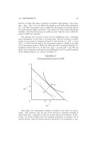
Figure 1.2 plots the expenditure components of GDP (as a ratio of GDP)
for the United States and Canada over the period 1961-2002. Once again, it is
1.2. HOW GDP IS CALCULATED 7
in teresting to note the relative stability of these ratios over long periods of time.
To a first approximation, it appears that private consumption expenditures (on
services and nondurables) constitute between 50—60% of GDP, private inv est-
men t expenditures constitute betw een 20—30% of GDP, government purchases
constitute between 20—25% of GDP, with NX averaging close to 0% over long
periods of time. Note, however, that in recent years, the United States has been
running a negative trade balance while Canada has been running a positive
trade balance.
0
20
40
60
80
100

65 70 75 80 85 90 95 00
Consumption
Investment
Government
Net Exports
Canada
0
20
40
60
80
100
65 70 75 80 85 90 95 00
Consumption
Investment
Government
Net Exports
United States
Percent of GDP
FIGURE 1.2
GDP Expenditure Components
United States and Canada
1961.1 - 2003.4
1.2.3 The Income-Expenditure Iden tit y
So far, we have established that GDP ≡ GDI and GDP ≡ GDE. From these
tw o equivalence relations, it follows that GDE ≡ GDI. In other words, aggre-
gate expenditure is equivalent to aggregate income, each of which are equivalent
to the value of aggregate production. One way to understand why this must be
true is as follows. First, any output that is produced must also be purchased
(additions to inventory are treated purchases of new capital goods, or invest-

ment spending). Hence the value of production must (by definition) be equal
to the value of spending. Second, since spending b y one individual constitutes
income for someone else, total spending must (by definition) be equal to total
income.
The identity GDI ≡ GDE is sometimes referred to as the income-expenditure
identity.LettingY denote the GDI, most introductory macroeconomic text-
books express the income-expenditure identity in the following way:
8 CHAPTER 1 . THE GROSS DOMESTIC PRODUCT
Y ≡ C + I + G + X − M.
Note that since the income-expenditure identity is an identity, it always
holds true. However, it is very important to understand what this identity does
and does not imply. A natural inclination is to suppose that since the identity
is always true, one can use it to make theoretical or predictive statements. For
example, the identity seems to suggest that an expansionary fiscal policy (an
increase in G) must necessarily result in an increase in GDP (an increase in Y ).
In fact, the income-expenditur e i dentity implies no such thing.
To understand why this is the case, what one must recognize is that an
iden tity is not a theory about the w ay the w orld works. In particular, the
income-expenditure identity is nothing more than a description of the world;
i.e., it is simply categorizes GDP into to its expenditure components and then
exploits the fact that total expenditure is by construction equivalent to total
income. To make predictions or offer interpretations of the data, one must
necessarily employ some type of theory. As we shall see later on, an increase in
G may or may not lead to an increase in Y , depending on circumstances. But
whether or not Y is predicted to rise or fall, the income-expenditure identity
will always hold true.
1.3 What GDP Does Not Measure
Before moving on, it is important to keep in mind what GDP does not measure
both in principle and in practice (i.e., things that should be counted as GDP in
principle, but may not be in practice).

In principle, GDP is supposed to measure the value of output that is in
some sense ‘marketable’ or ‘exchangeable’ (even if it is not actually marke ted or
exchanged). For example, if you spend 40 hours a week working in the market
sector, your earnings measure the market value of the output you produce.
However, there are 168 hours in a week. What are you producing with your
remaining 126 hours? Some of this time may be spent producing marketable
output that is not exc hanged in a market. Some examples here include the
time you spend doing housework, mowing the lawn, and repairing your car, etc.
Assuming that you do not like to do any of these things, you could contract
out these chores. If you did, what you pay for such services would be counted
as part of the GDP. But whether you contract out such services or not, they
clearly have value and this value should be counted as part of the GDP (even if
it is not always done so in practice).
The great majority of peoples’ time, however, appears to be employed in the
production of ‘nonmarketable’ output. Nonmarketable output may be either in
the form of consumption or investmen t . As a consumption good, a nonmar-
ketable output is an object that is simultaneously produced and consumed by
1.4. NOMINAL VERSUS REAL GDP 9
the individual producing it. An obvious example here is sleep (beyond what is
necessary to maintain one’s health). It is hard to get someone else to sleep for
you. A wide variety of leisure activities fall into this category as well (imagine
asking someone to go on vacation for you). As an investment good, a nonmar-
ketable output is an object that remains physically associated with the individ-
ual producing it. Time spent in school accumulating ‘human capital’ falls in to
this category.
2
A less obvious example may also include time spent searc hing
for work. Nonmarketable output is likely very large and obviously has value.
However, it is not c ounted as part of an economy’s GDP.
Another point to stress concerning GDP as a measure of ‘performance’ is

that it tells us nothing about the distribution of output in an economy. At best,
the (per capita) GDP can only give us some idea about the level of production
accruing to an ‘average’ individual in the economy.
Finally, it should be pointed out that there may be a branch of an economy’s
production flow should be counted as GDP in principle, but for a variety of
reasons, is not counted as such in practice. Ultimately, this problem stems with
the lack of information available to statistical agencies concerning the production
of ma rketable output that is either consumed by the producer or exchanged in
‘underground’ markets; see Appendix 1.A for d etails.
1.4 Nom inal versus Re al GD P
GDP was defined abo ve as the value of output (income or expenditure). The
definition did not, ho wever, specify in which units ‘value’ is to be measured. In
everyday life, the value of goods and services is usually stated in terms of market
prices measured in units of the national currency (e.g., Canadian dollars). For
example, the dozen bottles of beer you drank at last night’s student social cost
you $36 (and possibly a hangover). The 30 hours you worked last w eek cost
your employer $300; and so on. If we add up incomes and expenditures in t his
manner, we arrive at a GDP figure measured in units of money; this measure is
called the nominal GDP.
If market prices (including nominal exchange rates) remained constant over
time, then the nominal GDP w ould make comparisons of GDP across time
and countries an easy task (subject to the cav eats outlined in Appendix 1.A).
Unfortunately, as far as measurement issues are concerned, market prices do not
remain constant over time. So why is this a problem?
The value of either income or expenditure is measured as the product of
prices (measured in units of money) and quantities. It seems reasonable to
suppose that material living standards are somehow related to quantities; and
not the value of these quantities measured in money terms. In most economies
2
Note that while th e services of the hu m an capital accumulated in this way m ay subse-

quently b e rented out, the human capital itself remains emb edded in the individual’s brain.
As of this w riting, no technology exists that allows us to trade bits of our brain.
10 CHAPTER 1 . THE GROSS DOMESTIC PRODUCT
(with some notable exceptions), the general level of prices tends to grow over
time; such a phenomenon is known as inflation.Wheninflation is a feature
of the economic environment , the nominal GDP will rise even if the quantities
of production remain unchanged over time. For example, consider an economy
that produces nothing but bread and that year after year, bread production is
equal to 100 loaves. Suppose that the price of bread ten years ago was equal
to $1.00 per loaf, so that the nominal GDP then was equal to $100. Suppose
further that the price o f bread has risen by 10% per annum ov er the last ten
years. The nominal GDP after ten years is then given by (1.10)
10
($100) = $260.
Observ e that while the nominal GDP is 2.6 times higher than it was ten years
ago, the ‘real’ GDP (the stuff that people presumably care about) has remained
constant over time.
Thus, while measuring value in units of money is convenient, it is also prob-
lematic as far as measuring material living standards. But if we can no longer
rely on market prices denominated in money to give us a common unit of mea-
surement, then how are we to measure the value of an economy’s output? If an
economy simply produced one type of good (as in our example abo ve), then the
answer is simple: Measure value in units of the good produced (e.g., 100 loaves
of bread). In reality, ho wever, economies typically produce a wide assortment
of goods and services. It would make little s ense to simply add up the level of
individual quantities produced; for example, 100 loaves of bread, plus 3 tractors,
and 12 haircuts does not add up to anything that we can make sense of.
So we return to the question of how to measure ‘value.’ As it turns out, there
is no unique way to measure value. How one chooses to measure things depends
on the type of ‘ruler’ one a pplies to the measurement. For example, consider

the distance between New York and Paris. How does one measure distance? In
the United States, long distances are measured in ‘miles.’ T he distance betw een
New York and Paris is 3635 miles. In France, long distances are measured in
‘kilometers’. The distance between Paris and New York is 5851 kilometers.
Thankfully, there is a fixed ‘exchange rate’ between kilometers and miles (1
mile is approximately 1.6 kilometers), so that both measures provide the same
information. Just as importantly, there is a fixed exchange rate between miles
across time (one mile ten years ago is the same as one mile today).
The phenomenon of inflation (or deflation) distorts the length of our measur-
ing instrument (money) over time. Returning to our distance analogy, imagine
that the government decides to increase the distance in a mile by 10% per year.
While the distance between New York and Paris is currently 3635 miles, after
ten years this distance will have grown to (1.10)
10
(3635) = 9451 miles. Clearly,
the increase in distance here is just an illusion (the ‘real’ distance has remained
constant over time). Similarly, when there is an inflation, growth in the nom-
inal GDP will give the illusion of rising living standards, even if ‘real’ living
standards remain constant over time.
There are a number of different ways in which to deal with the measurement
issues in troduced by inflation. Here, I will simply describe one approach that is
1.4. NOMINAL VERSUS REAL GDP 11
commonly adopted by statistical agencies. Consider an economy that produces
n different goods and services. Let t denote the time-period (e.g., year) under
consideration. Let x
i
t
denote the quantity of good i produced at date t and
let p
i

t
denote the money price of good i produced at date t. Statistical agencies
collect information on the expenditures made on each domestically produced
good and service; i.e., p
i
t
x
i
t
, for i =1, 2, , n and for each year t. The gross
domestic expenditure (measured in current dollars) is simply given b y :
GDE
t
=
n
X
i=1
p
i
t
x
i
t
.
Now, choose one year arbitrarily (e.g., t = 1997) and call this the base
year. Then, the real GDP (RGDP) in any year t is calculated according to t he
following formula:
RGDP
t
≡

n
X
i=1
p
i
1997
x
i
t
.
This measure is called the GDP (expenditure based) in terms of base year (1997)
prices. In other words, the value of the GDP at date t is now measured in units
of 1997 dollars (instead of current, or date t dollars). Note that by construct i on,
RGDP
1997
= GDE
1997
.
As a by-product of this calculation, one can calculate the average level of
prices (technically, the GDP Deflator or simply, the price level ) P
t
according to
the formu la:
P
t
≡
GDE
t
RGDP
t

.
Note that the GDP deflator is simply an index number; i.e., it has no economic
meaning (in particular, note that P
1997
=1by construction). Nevertheless, the
GDP deflator is useful for making comparisons in the price level across time.
That is, even if P
1997
=1and P
1998
=1.10 individually have no meaning, we
can still compare these two numbers to make the statement that the price level
rose by 10% between the years 1997 and 1998.
The methodology just described above is not fool-proof. In particular, the
procedure of using base year prices to compute a measure of real GDP assumes
that the s tructure of relative prices remains constant over tim e. To the extent
that this is not true (it most certainly is not), then measures of the growth
rate in real GDP can depend on the arbitrary choice of the base year.
3
Finally,
it should be noted that making cross-country comparisons is complicated by
the fact that nominal exchange rates tend to fluctuate over time as well. In
principle, one can correct for variation in the exchange rate, but how well this
is accomplished in practice rem ains an open question.
3
Some st a tist ic a l ag e n c ie s h ave intro d u c e d vario us ‘chain- we ig htin g’ p rocedu r es t o mitig a te
this prob lem.
12 CHAPTER 1 . THE GROSS DOMESTIC PRODUCT
1.5 Real GDP A cross Time
Figure 1.3 plots the time path of real (i.e., corrected for inflation) per capita

GDP for the United States and Canada since the first quarter of 1961.
20000
24000
28000
32000
36000
40000
44000
48000
65 70 75 80 85 90 95 00
2000 US$ Per Annum
United States
8000
12000
16000
20000
24000
28000
32000
36000
65 70 75 80 85 90 95 00
1997 CDN$ Per Annum
Canada
FIGURE 1.3
Real per capita GDP
United States and Canada
1961.1 - 2003.4
The pattern of economic development for these two countries in Figure 1.3 is
typical of the pattern of development observed in many industrialized countries
ov er the last century and earlier. The most striking feature in Figure 1.3 is that

real per capita income tends to grow over time. Over the last 100 years, the rate
of growth in these two North American economies has averaged approximately
2% per annum.
Now, 2% per annum may not sound like a large number, but one should
keep in mind that even very low rates of growth can translate into very large
changes in the level of income over long periods of time. To see this, consider
the ‘rule of 72,’ which tells us the number of years n it would take to double
incomes if an economy grows a t rate of g% per annum:
n =
72
g
.
Thus, an economy growing at 2% per annum would lead to a doubling of income
every 36 years. In other words, we are roughly twice as rich as our predecessors
who lived here in 1967; and we are four times as r ich as those who lived here in
1931.
Since our current high living standards depend in large part on past growth,
and since our future living standards (and those of our children) will depend
on current and future growth rates, understanding the phenomenon of growth
is of primary importance. The branch of macroeconomics concerned with the
1.5. REAL GDP ACROSS TIME 13
issue of long-run growth is called growth theory. A closely related branch of
macroeconomics, which is concerned primarily with explaining the level and
growth of incomes across countries, is called development theory. We will discuss
theories of growth and development in the chapters ahead.
Traditionally, macroeconomics has been concerned more with the issue of
‘short run’ growth, or what is usually referred to as the business cycle.The
business cycle refers to the cyclical fluctuations in GDP around its ‘trend,’
where trend may defined e ither in terms of levels or growth rates. From Figure
1.3, we see that while per capita GDP tends to rise over long periods of time,

the rate of growth over short periods of time can fluctuate substantially. In fact,
there appear to be (relatively brief) periods of time when the real GDP actually
falls (i.e., the growth rate is negative). When the real GDP falls for two or
more consecutive quarters (six mon ths), the economy is said to be in recession.
Figure 1.4 plots the growth rate in real per capita GDP for the United States
and Canada.
-8
-6
-4
-2
0
2
4
6
8
65 70 75 80 85 90 95 00
U.S. Canada
FIGURE 1.4
Growth Rate in Real Per Capita GDP
(5-quarter moving average)
Percent per Annum
Figure 1.4 reveals that the cyclical pattern of GDP growth in the United
States and Canada are similar, but not identical. In particular, note that
Canada largely escaped the three significant rec essions that afflicted the U.S.
during the 1970s (although growth did slow down in Canada during these