AUTOMATION & CONTROL - Theory and Practice Part 1 ppt
Bạn đang xem bản rút gọn của tài liệu. Xem và tải ngay bản đầy đủ của tài liệu tại đây (864.93 KB, 25 trang )
I
AUTOMATION & CONTROL
- Theory and Practice
AUTOMATION & CONTROL
- Theory and Practice
Edited by
A. D. Rodić
In-Tech
intechweb.org
Published by In-Teh
In-Teh
Olajnica 19/2, 32000 Vukovar, Croatia
Abstracting and non-prot use of the material is permitted with credit to the source. Statements and
opinions expressed in the chapters are these of the individual contributors and not necessarily those of
the editors or publisher. No responsibility is accepted for the accuracy of information contained in the
published articles. Publisher assumes no responsibility liability for any damage or injury to persons or
property arising out of the use of any materials, instructions, methods or ideas contained inside. After
this work has been published by the In-Teh, authors have the right to republish it, in whole or part, in any
publication of which they are an author or editor, and the make other personal use of the work.
© 2009 In-teh
www.intechweb.org
Additional copies can be obtained from:
First published December 2009
Printed in India
Technical Editor: Melita Horvat
AUTOMATION & CONTROL - Theory and Practice,
Edited by A. D. Rodić
p. cm.
ISBN 978-953-307-039-1
V
Preface
Automation is the use of control systems (such as numerical control, programmable
logic control, and other industrial control systems), in concert with other applications of
information technology (such as computer-aided technologies [CAD, CAM, CAx]), to control
industrial machinery and processes, reducing the need for human intervention. In the scope
of industrialization, automation is a step beyond mechanization. Whereas mechanization
provided human operators with machinery to assist them with the muscular requirements of
work, automation greatly reduces the need for human sensory and mental requirements as
well. Processes and systems can also be automated.
Automation plays an increasingly important role in the global economy and in daily experience.
Engineers strive to combine automated devices with mathematical and organizational tools to
create complex systems for a rapidly expanding range of applications and human activities.
Many roles for humans in industrial processes presently lie beyond the scope of automation.
Human-level pattern recognition, language recognition, and language production ability are
well beyond the capabilities of modern mechanical and computer systems. Tasks requiring
subjective assessment or synthesis of complex sensory data, such as scents and sounds, as
well as high-level tasks such as strategic planning, currently require human expertise. In
many cases, the use of humans is more cost-effective than mechanical approaches even where
automation of industrial tasks is possible.
Specialized industrial computers, referred to as programmable logic controllers (PLCs), are
frequently used to synchronize the ow of inputs from (physical) sensors and events with the
ow of outputs to actuators and events. This leads to precisely controlled actions that permit
a tight control of almost any industrial process.
Human-machine interfaces (HMI) or computer human interfaces (CHI), formerly known
as man-machine interfaces, are usually employed to communicate with PLCs and other
computers, such as entering and monitoring temperatures or pressures for further automated
control or emergency response. Service personnel who monitor and control these interfaces
are often referred to as stationary engineers.
Different types of automation tools exist:
• ANN - Articial neural network
• DCS - Distributed Control System
• HMI - Human Machine Interface
• SCADA - Supervisory Control and Data Acquisition
VI
• PLC - Programmable Logic Controller
• PAC - Programmable Automation Controller
• Instrumentation
• Motion control
• Robotics
Control theory is an interdisciplinary branch of engineering and mathematics that deals with
the behavior of dynamical systems. Control theory is
• a theory that deals with inuencing the behavior of dynamical systems
• an interdisciplinary subeld of science, which originated in engineering and mathematics,
and evolved into use by the social, economic and other sciences.
Main control techniques assume:
• Adaptive control uses on-line identication of the process parameters, or modication of
controller gains, thereby obtaining strong robustness properties.
• A Hierarchical control system is a type of Control System in which a set of devices and
governing software is arranged in a hierarchical tree. When the links in the tree are
implemented by a computer network, then that hierarchical control system is also a form
of a Networked control system.
• Intelligent control use various AI computing approaches like neural networks, Bayesian
probability, fuzzy logic, machine learning, evolutionary computation and genetic
algorithms to control a dynamic system.
• Optimal control is a particular control technique in which the control signal optimizes
a certain “cost index”. Two optimal control design methods have been widely used in
industrial applications, as it has been shown they can guarantee closed-loop stability.
These are Model Predictive Control (MPC) and Linear-Quadratic-Gaussian control (LQG).
• Robust control deals explicitly with uncertainty in its approach to controller design.
Controllers designed using robust control methods tend to be able to cope with small
differences between the true system and the nominal model used for design.
• Stochastic control deals with control design with uncertainty in the model. In typical
stochastic control problems, it is assumed that there exist random noise and disturbances
in the model and the controller, and the control design must take into account these
random deviations.
The present edited book is a collection of 18 chapters written by internationally recognized
experts and well-known professionals of the eld. Chapters contribute to diverse facets of
automation and control. The volume is organized in four parts according to the main subjects,
regarding the recent advances in this eld of engineering.
The rst thematic part of the book is devoted to automation. This includes solving of assembly
line balancing problem and design of software architecture for cognitive assembling in
production systems.
The second part of the book concerns with different aspects of modeling and control. This
includes a study on modeling pollutant emission of diesel engine, development of a PLC program
obtained from DEVS model, control networks for digital home, automatic control of temperature
and ow in heat exchanger, and non-linear analysis and design of phase locked loops.
VII
The third part addresses issues of parameter estimation and lter design, including methods
for parameters estimation, control and design of the wave digital lters.
The fourth part presents new results in the intelligent control. That includes building of a
neural PDF strategy for hydroelectric station simulator, intelligent network system for
process control, neural generalized predictive control for industrial processes, intelligent
system for forecasting, diagnosis and decision making based on neural networks and self-
organizing maps, development of a smart semantic middleware for the Internet , development
appropriate AI methods in fault-tolerant control, building expert system in rotary railcar
dumpers, expert system for plant asset management, and building of a image retrieval system
in heterogeneous database.
The content of this thematic book admirably reects the complementary aspects of theory
and practice which have taken place in the last years. Certainly, the content of this book will
serve as a valuable overview of theoretical and practical methods in control and automation
to those who deal with engineering and research in this eld of activities.
The editors are greatfull to the authors for their excellent work and interesting contributions.
Thanks are also due to the renomeus publisher for their editorial assistance and excellent
technical arrangement of the book.
December, 2009
A. D. Rodić
IX
Contents
Preface V
I. Automation
1. AssemblyLineBalancingProblemSingleandTwo-SidedStructures 001
WaldemarGrzechca
2. ASoftwareArchitectureforCognitiveTechnicalSystemsSuitableforan
AssemblyTaskinaProductionEnvironment 013
EckartHauck,ArnoGramatkeandKlausHenning
II. Modeling and Control
3. Twostageapproachesformodelingpollutantemissionofdieselenginebasedon
Krigingmodel 029
ElHassaneBrahmi,LilianneDenis-Vidal,ZohraCher,NassimBoudaoudandGhislaine
Joly-Blanchard
4. AnapproachtoobtainaPLCprogramfromaDEVSmodel 047
HyeongT.Park,KilY.Seong,SurajDangol,GiN.WangandSangC.Park
5. Aframeworkforsimulatinghomecontrolnetworks 059
RafaelJ.Valdivieso-Sarabia,JorgeAzorín-López,AndrésFuster-GuillóandJuanM.García-
Chamizo
6. ComparisonofDefuzzicationMethods:AutomaticControlofTemperatureand
FlowinHeatExchanger 077
AlvaroJ.ReyAmaya,OmarLengerke,CarlosA.Cosenza,MaxSuellDutraandMagda
J.M.Tavera
7. NonlinearAnalysisandDesignofPhase-LockedLoops 089
G.A.Leonov,N.V.KuznetsovandS.M.Seledzhi
III. Estimation and Filter Design
8. Methodsforparameterestimationandfrequencycontrolofpiezoelectric
transducers 115
ConstantinVolosencu
9. DesignoftheWaveDigitalFilters 137
BohumilPsenicka,FranciscoGarcíaUgaldeandAndrésRomeroM.
X
IV. Intelligent Control
10. NeuralPDFControlStrategyforaHydroelectricStationSimulator 161
GermanA.Munoz-Hernandez,CarlosA.Gracios-Marin,AlejandroDiaz-Sanchez,SaadP.
MansoorandDewiI.Jones
11. IntelligentNetworkSystemforProcessControl:Applications,Challenges,
Approaches 177
QurbanAMemon
12. NeuralGeneralizedPredictiveControlforIndustrialProcesses 199
SadhanaChidrawar,BalasahebPatreandLaxmanWaghmare
13. Forecasting,DiagnosisandDecisionMakingwithNeuralNetworksand
Self-OrganizingMaps 231
KazuhiroKohara,KatsuyoshiAokiandMamoruIsomae
14. ChallengesofMiddlewarefortheInternetofThings 247
MichalNagy,ArtemKatasonov,OleksiyKhriyenko,SergiyNikitin,MichalSzydłowskiand
VaganTerziyan
15. ArticialIntelligenceMethodsinFaultTolerantControl 271
LuisE.GarzaCastañónandAdrianaVargasMartínez
16. ARealTimeExpertSystemForDecisionMakinginRotaryRailcarDumpers 297
OsevaldoFarias,SoaneLabidi,JoãoFonsecaNeto,JoséMouraandSamyAlbuquerque
17. ModularandHybridExpertSystemforPlantAssetManagement 311
MarioThronandNicoSuchold
18. ImageRetrievalSysteminHeterogeneousDatabase 327
KhalifaDjemal,HichemMaarefandRostomKachouri
AssemblyLineBalancingProblemSingleandTwo-SidedStructures 1
AssemblyLineBalancingProblemSingleandTwo-SidedStructures
WaldemarGrzechca
X
Assembly Line Balancing Problem
Single and Two-Sided Structures
Waldemar Grzechca
The Silesian University of Technology
Poland
1. Introduction
The manufacturing assembly line was first introduced by Henry Ford in the early 1900’s. It
was designed to be an efficient, highly productive way of manufacturing a particular
product. The basic assembly line consists of a set of workstations arranged in a linear
fashion, with each station connected by a material handling device. The basic movement of
material through an assembly line begins with a part being fed into the first station at
a predetermined feed rate. A station is considered any point on the assembly line in which
a task is performed on the part. These tasks can be performed by machinery, robots, and/or
human operators. Once the part enters a station, a task is then performed on the part, and
the part is fed to the next operation. The time it takes to complete a task at each operation is
known as the process time (Sury, 1971). The cycle time of an assembly line is predetermined
by a desired production rate. This production rate is set so that the desired amount of end
product is produced within a certain time period (Baybars, 1986). In order for the assembly
line to maintain a certain production rate, the sum of the processing times at each station
must not exceed the station’s cycle time (Fonseca et al, 2005). If the sum of the processing
times within a station is less than the cycle time, idle time is said to be present at that station
(Erel et al,1998). One of the main issues concerning the development of an assembly line is
how to arrange the tasks to be performed. This arrangement may be somewhat subjective,
but has to be dictated by implied rules set forth by the production sequence (Kao, 1976). For
the manufacturing of any item, there are some sequences of tasks that must be followed. The
assembly line balancing problem (ALBP) originated with the invention of the assembly line.
Helgeson et al (Helgeson et al, 1961) were the first to propose the ALBP, and Salveson
(Salveson, 1955) was the first to publish the problem in its mathematical form. However,
during the first forty years of the assembly line’s existence, only trial-and-error methods
were used to balance the lines (Erel et al,, 1998). Since then, there have been numerous
methods developed to solve the different forms of the ALBP. Salveson (Salveson, 1955)
provided the first mathematical attempt by solving the problem as a linear program. Gutjahr
and Nemhauser (Gutjahr & Nemhauser, 1964) showed that the ALBP problem falls into the
class of NP-hard combinatorial optimization problems. This means that an optimal solution
is not guaranteed for problems of significant size. Therefore, heuristic methods have become
the most popular techniques for solving the problem. Author of this book chapter
1
AUTOMATION&CONTROL-TheoryandPractice2
underlines the importance of the final results estimation and proposes for single and two-
sided assembly line balancing problem modified measures.
2. Two-sided Assembly Lines
Two-sided assembly lines (Fig. 1.) are typically found in producing large-sized products,
such as trucks and buses. Assembling these products is in some respects different from
assembling small products. Some assembly operations prefer to be performed at one of the
two sides (Bartholdi, 1993).
Fig. 1. Two-sided assembly line structure
Let us consider, for example, a truck assembly line. Installing a gas tank, air filter, and
toolbox can be more easily achieved at the left-hand side of the line, whereas mounting
a battery, air tank, and muffler prefers the right-hand side. Assembling an axle, propeller
shaft, and radiator does not have any preference in their operation directions so that they
can be done at any side of the line. The consideration of the preferred operation directions is
important since it can greatly influence the productivity of the line, in particular when
assigning tasks, laying out facilities, and placing tools and fixtures in a two-sided assembly
line (Kim et al, 2001). A two-sided assembly line in practice can provide several substantial
advantages over a one-sided assembly line (Bartholdi, 1993). These include the following: (1)
it can shorten the line length, which means that fewer workers are required, (2) it thus can
reduce the amount of throughput time, (3) it can also benefit from lowered cost of tools and
fixtures since they can be shared by both sides of a mated-station, and (4) it can reduce
material handling, workers movement and set-up time, which otherwise may not be easily
eliminated. These advantages give a good reason for utilizing two-sided lines for
assembling large-sized products. A line balancing problem is usually represented by
a precedence diagram as illustrated in Fig. 2.
Fig. 2. Precedence graph
Station n
Conveyor
Station 1 Station 3
Station (n-2) Station 4 Station 2
Station (n-3) Station (n-1)
1
4
5
2
3
6
7
8
9
10
11
12
(4, L)
(5 , E )
(3, R )
(6 , L )
(4, E )
(4, R )
(5, L )
(4, E ) (5, E )
(8, E )
(7, E )
(1, R )
A circle indicates a task, and an arc linking two tasks represents the precedence relation
between the tasks. Each task is associated with a label of (t
i
, d), where t
i
is the task processing
time and d (=L, R or E) is the preferred operation direction. L and R, respectively, indicate
that the task should be assigned to a left- and a right-side station. A task associated with E
can be performed at either side of the line. While balancing assembly lines, it is generally
needed to take account of the features specific to the lines. In a one-sided assembly line, if
precedence relations are considered appropriately, all the tasks assigned to a station can be
carried out continuously without any interruption. However, in a two-sided assembly line,
some tasks assigned to a station can be delayed by the tasks assigned to its companion
(Bartholdi, 1993). In other words, idle time is sometimes unavoidable even between tasks
assigned to the same station. Consider, for example, task j and its immediate predecessor i.
Suppose that j is assigned to a station and i to its companion station. Task j cannot be started
until task i is completed. Therefore, balancing such a two-sided assembly line, unlike a one-
sided assembly line, needs to consider the sequence-dependent finish time of tasks.
3. Heuristic Methods in Assembly Line Balancing Problem
The heuristic approach bases on logic and common sense rather than on mathematical
proof. Heuristics do not guarantee an optimal solution, but results in good feasible solutions
which approach the true optimum.
3.1 Single Assembly Line Balancing Heuristic Methods
Most of the described heuristic solutions in literature are the ones designed for solving
single assembly line balancing problem. Moreover, most of them are based on simple
priority rules (constructive methods) and generate one or a few feasible solutions. Task-
oriented procedures choose the highest priority task from the list of available tasks and
assign it to the earliest station which is assignable. Among task-oriented procedures we can
distinguish immediate-update-first-fit (IUFF) and general-first-fit methods depending on
whether the set of available tasks is updated immediately after assigning a task or after the
assigning of all currently available tasks. Due to its greater flexibility immediate-update-
first-fit method is used more frequently. The main idea behind this heuristic is assigning
tasks to stations basing on the numerical score. There are several ways to determine
(calculate) the score for each tasks. One could easily create his own way of determining the
score, but it is not obvious if it yields good result. In the following section five different
methods found in the literature are presented along with the solution they give for our
simple example. The methods are implemented in the Line Balancing program as well.
From the moment the appropriate score for each task is determined there is no difference in
execution of methods and the required steps to obtain the solution are as follows:
STEP 1. Assign a numerical score n(x) to each task x.
STEP 2. Update the set of available tasks (those whose immediate predecessors have been
already assigned).
STEP 3. Among the available tasks, assign the task with the highest numerical score to the
first station in which the capacity and precedence constraints will not be violated. Go to
STEP 2.
The most popular heuristics which belongs to IUFF group are:
IUFF-RPW Immediate Update First Fit – Ranked Positional Weight,
AssemblyLineBalancingProblemSingleandTwo-SidedStructures 3
underlines the importance of the final results estimation and proposes for single and two-
sided assembly line balancing problem modified measures.
2. Two-sided Assembly Lines
Two-sided assembly lines (Fig. 1.) are typically found in producing large-sized products,
such as trucks and buses. Assembling these products is in some respects different from
assembling small products. Some assembly operations prefer to be performed at one of the
two sides (Bartholdi, 1993).
Fig. 1. Two-sided assembly line structure
Let us consider, for example, a truck assembly line. Installing a gas tank, air filter, and
toolbox can be more easily achieved at the left-hand side of the line, whereas mounting
a battery, air tank, and muffler prefers the right-hand side. Assembling an axle, propeller
shaft, and radiator does not have any preference in their operation directions so that they
can be done at any side of the line. The consideration of the preferred operation directions is
important since it can greatly influence the productivity of the line, in particular when
assigning tasks, laying out facilities, and placing tools and fixtures in a two-sided assembly
line (Kim et al, 2001). A two-sided assembly line in practice can provide several substantial
advantages over a one-sided assembly line (Bartholdi, 1993). These include the following: (1)
it can shorten the line length, which means that fewer workers are required, (2) it thus can
reduce the amount of throughput time, (3) it can also benefit from lowered cost of tools and
fixtures since they can be shared by both sides of a mated-station, and (4) it can reduce
material handling, workers movement and set-up time, which otherwise may not be easily
eliminated. These advantages give a good reason for utilizing two-sided lines for
assembling large-sized products. A line balancing problem is usually represented by
a precedence diagram as illustrated in Fig. 2.
Fig. 2. Precedence graph
Station n
Conveyor
Station 1 Station 3
Station (n-2) Station 4 Station 2
Station (n-3) Station (n-1)
1
4
5
2
3
6
7
8
9
10
11
12
(4, L)
(5 , E )
(3, R )
(6 , L )
(4, E )
(4, R )
(5, L )
(4, E ) (5, E )
(8, E )
(7, E )
(1, R )
A circle indicates a task, and an arc linking two tasks represents the precedence relation
between the tasks. Each task is associated with a label of (t
i
, d), where t
i
is the task processing
time and d (=L, R or E) is the preferred operation direction. L and R, respectively, indicate
that the task should be assigned to a left- and a right-side station. A task associated with E
can be performed at either side of the line. While balancing assembly lines, it is generally
needed to take account of the features specific to the lines. In a one-sided assembly line, if
precedence relations are considered appropriately, all the tasks assigned to a station can be
carried out continuously without any interruption. However, in a two-sided assembly line,
some tasks assigned to a station can be delayed by the tasks assigned to its companion
(Bartholdi, 1993). In other words, idle time is sometimes unavoidable even between tasks
assigned to the same station. Consider, for example, task j and its immediate predecessor i.
Suppose that j is assigned to a station and i to its companion station. Task j cannot be started
until task i is completed. Therefore, balancing such a two-sided assembly line, unlike a one-
sided assembly line, needs to consider the sequence-dependent finish time of tasks.
3. Heuristic Methods in Assembly Line Balancing Problem
The heuristic approach bases on logic and common sense rather than on mathematical
proof. Heuristics do not guarantee an optimal solution, but results in good feasible solutions
which approach the true optimum.
3.1 Single Assembly Line Balancing Heuristic Methods
Most of the described heuristic solutions in literature are the ones designed for solving
single assembly line balancing problem. Moreover, most of them are based on simple
priority rules (constructive methods) and generate one or a few feasible solutions. Task-
oriented procedures choose the highest priority task from the list of available tasks and
assign it to the earliest station which is assignable. Among task-oriented procedures we can
distinguish immediate-update-first-fit (IUFF) and general-first-fit methods depending on
whether the set of available tasks is updated immediately after assigning a task or after the
assigning of all currently available tasks. Due to its greater flexibility immediate-update-
first-fit method is used more frequently. The main idea behind this heuristic is assigning
tasks to stations basing on the numerical score. There are several ways to determine
(calculate) the score for each tasks. One could easily create his own way of determining the
score, but it is not obvious if it yields good result. In the following section five different
methods found in the literature are presented along with the solution they give for our
simple example. The methods are implemented in the Line Balancing program as well.
From the moment the appropriate score for each task is determined there is no difference in
execution of methods and the required steps to obtain the solution are as follows:
STEP 1. Assign a numerical score n(x) to each task x.
STEP 2. Update the set of available tasks (those whose immediate predecessors have been
already assigned).
STEP 3. Among the available tasks, assign the task with the highest numerical score to the
first station in which the capacity and precedence constraints will not be violated. Go to
STEP 2.
The most popular heuristics which belongs to IUFF group are:
IUFF-RPW Immediate Update First Fit – Ranked Positional Weight,
AUTOMATION&CONTROL-TheoryandPractice4
IUFF-NOF Immediate Update First Fit – Number of Followers,
IUFF-NOIF Immediate Update First Fit – Number of Immediate Followers,
IUFF-NOP Immediate Update First Fit – Number of Predecessors,
IUFF-WET Immediate Update First Fit – Work Element Time.
3.2 Two-sided Assembly Line Balancing Heuristic Method
A task group consists of a considered task i and all of its predecessors. Such groups are
generated for every un–assigned task. As mentioned earlier, balancing a two–sided
assembly line needs to additionally consider operation directions and sequence dependency
of tasks, while creating new groups (Lee et al, 2001). While forming initial groups IG(i), the
operation direction is being checked all the time. It’s disallowed for a group to contain tasks
with preferred operation direction from opposite sides. But, if each task in initial group is E
– task, the group can be allocated to any side. In order to determine the operation directions
for such groups, the rules (direction rules DR) are applied:
DR 1. Set the operation direction to the side where tasks can be started earlier.
DR 2. The start time at both sides is the same, set the operation direction to the side where
it’s expected to carry out a less amount of tasks (total operation time of unassigned L or R
tasks).
Generally, tasks resulting from “repeatability test” are treated as starting ones. But there is
exception in form of first iteration, where procedure starts from searching tasks (initial tasks
IT), which are the first ones in precedence relation. After the first step in the first iteration
we get:
IG (1) = {1}, Time{IG (1)} = 2, Side{IG (1)} = ‘L’
IG (2) = {2}, Time{IG (2)} = 5, Side{IG (2)} = ‘E’
IG (3) = {3}, Time{IG (3)} = 3, Side{IG (3)} = ‘R
where:
Time{IG(i)} – total processing time of i
th
initial group,
Side{IG(i)} – preference side of i
th
initial group.
To those who are considered to be the first, the next tasks will be added, (these ones which
fulfil precedence constraints).
Whenever new tasks are inserted to the group i, the direction, cycle time and number of
immediate predecessors are checked. If there are more predecessors than one, the creation of
initial group j comes to the end.
First iteration – second step
IG (1) = {1, 4, 6}, Time{IG (1)} = 8, Side{IG (1)} = ‘L’
IG (2) = {2, 5}, Time{IG (2)} = 9 , Side{IG (2)} = ‘E’
IG (3) = {3, 5} , Time{IG (3)} = 7 , Side{IG (3)} = ‘R’
When set of initial groups is created, the last elements from those groups are tested for
repeatability. If last element in set of initial groups IG will occur more than once (groups
pointed by arrows), the groups are intended to be joined – if total processing time (summary
time of considered groups) is less or equal to cycle time. Otherwise, these elements are
deleted.
In case of occurring only once, the last member is being checked if its predecessors are not
contained in Final set FS. If not, it’s removed as well. So far, FS is empty.
First iteration – third step
IG (1) = {1, 4}, Time{IG (1)} = 4, Side{IG (1)} = ‘L’
IG (2) = {2, 3, 5}, Time{IG (2)} = 12, Side{IG (2)} = ‘R’
Whenever two or more initial groups are joined together, or when initial group is connected
with those one coming from Final set – the “double task” is added to initial tasks needed for
the next iteration. In the end of each iteration, created initial groups are copied to FS.
First iteration – fourth step
FS = { (1, 4); (2, 3, 5) },
Side{FS (1)} = ‘L’, Side{FS (2)} = ‘R’
Time {FS(2)} = 12, Time {FS(1)} = 14,
IT = {5}.
In the second iteration, second step, we may notice that predecessor of last task coming from
IG(1) is included in Final Set, FS(2). The situation results in connecting both groups under
holding additional conditions:
Side{IG(1)} = Side{FS(2)},
Time + time < cycle.
After all, there is no more IT tasks, hence, preliminary process of creating final set is
terminated.
The presented method for finding task groups is to be summarized in simplified algorithm
form. Let U denote to be the set of un – assigned tasks yet and IG
i
be a task group consisting
of task i and all its predecessors (excluded from U set).
STEP 1. If U = empty, go to step 5, otherwise, assign starting task from U.
STEP 2. Identify IG
i
. Check if it contains tasks with both left and right preference operation
direction, then remove task i.
STEP 3. Assign operation direction Side{ IG
i
} of group IG
i
. If IG
i
has R-task (L-task ), set the
operation direction to right (left). Otherwise, apply so called direction rules DR.
STEP 4. If the last task i in IG
i
is completed within cycle time, the IG
i
is added to Final set of
candidates FS(i). Otherwise, exclude task i from IG
i
and go to step 1.
STEP 5. For every task group in FS(i), remove it from FS if it is contained within another task
group of FS.
The resulting task groups become candidates for the mated-station
FS = {(1,4), (2,3,5,8)}.
The candidates are produced by procedures presented in the previous section, which claim
to not violate precedence, operation direction restrictions, and what’s more it exerts on
groups to be completed within preliminary determined cycle time. Though, all of candidates
may be assigned equally, the only one group may be chosen. Which group it will be – for
this purpose the rules helpful in making decision, will be defined and explained below:
AR 1. Choose the task group FS(i) that may start at the earliest time.
AR 2. Choose the task group FS(i) that involves the minimum delay.
AR 3. Choose the task group FS(i) that has the maximum processing time.
In theory, for better understanding, we will consider a left and right side of mated – station,
with some tasks already allocated to both sides. In order to achieve well balanced station,
the AR 1 is applied, cause the unbalanced station is stated as the one which would probably
involve more delay in future assignment. This is the reason, why minimization number of
stations is not the only goal, there are also indirect ones, such as reduction of unavoidable
delay. This rule gives higher priority to the station, where less tasks are allocated. If ties
occurs, the AR 2 is executed, which chooses the group with the least amount of delay among
the considered ones. This rule may also result in tie. The last one, points at relating work
AssemblyLineBalancingProblemSingleandTwo-SidedStructures 5
IUFF-NOF Immediate Update First Fit – Number of Followers,
IUFF-NOIF Immediate Update First Fit – Number of Immediate Followers,
IUFF-NOP Immediate Update First Fit – Number of Predecessors,
IUFF-WET Immediate Update First Fit – Work Element Time.
3.2 Two-sided Assembly Line Balancing Heuristic Method
A task group consists of a considered task i and all of its predecessors. Such groups are
generated for every un–assigned task. As mentioned earlier, balancing a two–sided
assembly line needs to additionally consider operation directions and sequence dependency
of tasks, while creating new groups (Lee et al, 2001). While forming initial groups IG(i), the
operation direction is being checked all the time. It’s disallowed for a group to contain tasks
with preferred operation direction from opposite sides. But, if each task in initial group is E
– task, the group can be allocated to any side. In order to determine the operation directions
for such groups, the rules (direction rules DR) are applied:
DR 1. Set the operation direction to the side where tasks can be started earlier.
DR 2. The start time at both sides is the same, set the operation direction to the side where
it’s expected to carry out a less amount of tasks (total operation time of unassigned L or R
tasks).
Generally, tasks resulting from “repeatability test” are treated as starting ones. But there is
exception in form of first iteration, where procedure starts from searching tasks (initial tasks
IT), which are the first ones in precedence relation. After the first step in the first iteration
we get:
IG (1) = {1}, Time{IG (1)} = 2, Side{IG (1)} = ‘L’
IG (2) = {2}, Time{IG (2)} = 5, Side{IG (2)} = ‘E’
IG (3) = {3}, Time{IG (3)} = 3, Side{IG (3)} = ‘R
where:
Time{IG(i)} – total processing time of i
th
initial group,
Side{IG(i)} – preference side of i
th
initial group.
To those who are considered to be the first, the next tasks will be added, (these ones which
fulfil precedence constraints).
Whenever new tasks are inserted to the group i, the direction, cycle time and number of
immediate predecessors are checked. If there are more predecessors than one, the creation of
initial group j comes to the end.
First iteration – second step
IG (1) = {1, 4, 6}, Time{IG (1)} = 8, Side{IG (1)} = ‘L’
IG (2) = {2, 5}, Time{IG (2)} = 9 , Side{IG (2)} = ‘E’
IG (3) = {3, 5} , Time{IG (3)} = 7 , Side{IG (3)} = ‘R’
When set of initial groups is created, the last elements from those groups are tested for
repeatability. If last element in set of initial groups IG will occur more than once (groups
pointed by arrows), the groups are intended to be joined – if total processing time (summary
time of considered groups) is less or equal to cycle time. Otherwise, these elements are
deleted.
In case of occurring only once, the last member is being checked if its predecessors are not
contained in Final set FS. If not, it’s removed as well. So far, FS is empty.
First iteration – third step
IG (1) = {1, 4}, Time{IG (1)} = 4, Side{IG (1)} = ‘L’
IG (2) = {2, 3, 5}, Time{IG (2)} = 12, Side{IG (2)} = ‘R’
Whenever two or more initial groups are joined together, or when initial group is connected
with those one coming from Final set – the “double task” is added to initial tasks needed for
the next iteration. In the end of each iteration, created initial groups are copied to FS.
First iteration – fourth step
FS = { (1, 4); (2, 3, 5) },
Side{FS (1)} = ‘L’, Side{FS (2)} = ‘R’
Time {FS(2)} = 12, Time {FS(1)} = 14,
IT = {5}.
In the second iteration, second step, we may notice that predecessor of last task coming from
IG(1) is included in Final Set, FS(2). The situation results in connecting both groups under
holding additional conditions:
Side{IG(1)} = Side{FS(2)},
Time + time < cycle.
After all, there is no more IT tasks, hence, preliminary process of creating final set is
terminated.
The presented method for finding task groups is to be summarized in simplified algorithm
form. Let U denote to be the set of un – assigned tasks yet and IG
i
be a task group consisting
of task i and all its predecessors (excluded from U set).
STEP 1. If U = empty, go to step 5, otherwise, assign starting task from U.
STEP 2. Identify IG
i
. Check if it contains tasks with both left and right preference operation
direction, then remove task i.
STEP 3. Assign operation direction Side{ IG
i
} of group IG
i
. If IG
i
has R-task (L-task ), set the
operation direction to right (left). Otherwise, apply so called direction rules DR.
STEP 4. If the last task i in IG
i
is completed within cycle time, the IG
i
is added to Final set of
candidates FS(i). Otherwise, exclude task i from IG
i
and go to step 1.
STEP 5. For every task group in FS(i), remove it from FS if it is contained within another task
group of FS.
The resulting task groups become candidates for the mated-station
FS = {(1,4), (2,3,5,8)}.
The candidates are produced by procedures presented in the previous section, which claim
to not violate precedence, operation direction restrictions, and what’s more it exerts on
groups to be completed within preliminary determined cycle time. Though, all of candidates
may be assigned equally, the only one group may be chosen. Which group it will be – for
this purpose the rules helpful in making decision, will be defined and explained below:
AR 1. Choose the task group FS(i) that may start at the earliest time.
AR 2. Choose the task group FS(i) that involves the minimum delay.
AR 3. Choose the task group FS(i) that has the maximum processing time.
In theory, for better understanding, we will consider a left and right side of mated – station,
with some tasks already allocated to both sides. In order to achieve well balanced station,
the AR 1 is applied, cause the unbalanced station is stated as the one which would probably
involve more delay in future assignment. This is the reason, why minimization number of
stations is not the only goal, there are also indirect ones, such as reduction of unavoidable
delay. This rule gives higher priority to the station, where less tasks are allocated. If ties
occurs, the AR 2 is executed, which chooses the group with the least amount of delay among
the considered ones. This rule may also result in tie. The last one, points at relating work
AUTOMATION&CONTROL-TheoryandPractice6
within individual station group by choosing group of task with highest processing time. For
the third rule the tie situation is impossible to obtain, because of random selection of tasks.
The implementation of above rules is strict and easy except the second one. Shortly
speaking, second rule is based on the test, which checks each task consecutively, coming
from candidates group FS(i) – in order to see if one of its predecessors have already been
allocated to station. If it has, the difference between starting time of considered task and
finished time of its predecessor allocated to companion station is calculated. The result
should be positive, otherwise time delay occurs.
Having rules for initial grouping and assigning tasks described in previous sections, we
may proceed to formulate formal procedure of solving two – sided assembly line balancing
problem (Kim et. al, 2005).
Let us denote companion stations as j and j’,
D(i) – the amount of delay,
Time(i) – total processing time (Time{FS(i)}),
S(j) – start time at station j,
STEP 1. Set up j = 1, j’ = j + 1, S(j) = S(j’) = 0, U – the set of tasks to be assigned.
STEP 2. Start procedure of group creating (3.2), which identifies
FS = {FS(1), FS(2), …, FS(n)}. If FS = , go to step 6.
STEP 3. For every FS(i), i = 1,2, … , n – compute D(i) and Time(i).
STEP 4. Identify one task group FS(i), using AR rules in Section 3.3
STEP 5. Assign FS(i) to a station j (j’) according to its operation direction, and update S(j) =
S(j) + Time(i) + D(i). U = U – {FS(i)}, and go to STEP 2.
STEP 6. If U
, set j = j’ + 1, j’ = j + 1, S(j) = S(j’) = 0, and go to STEP 2, otherwise, stop the
procedure.
4. Measures of Final Results of Assembly Line Balancing Problem
Some measures of solution quality have appeared in line balancing problem. Below are
presented three of them (Scholl, 1999).
Line efficiency (LE) shows the percentage utilization of the line. It is expressed as ratio of
total station time to the cycle time multiplied by the number of workstations:
100%
Kc
ST
LE
K
1i
i
(1)
where: K - total number of workstations,
c - cycle time.
Smoothness index (SI) describes relative smoothness for a given assembly line balance.
Perfect balance is indicated by smoothness index 0. This index is calculated in the following
manner:
K
1i
2
imax
STSTSI
(2)
where:
ST
max
- maximum station time (in most cases cycle time),
ST
i
- station time of station i.
Time of the line (LT) describes the period of time which is need for the product to be
completed on an assembly line:
K
T1KcLT
(3)
where:
c - cycle time,
K -total number of workstations,
T
K
– processing time of last station.
The final result estimation of two-sided assembly line balance needs some modification of
existing measures (Grzechca, 2008).
Time of line for TALBP
K K 1
LT c Km 1 Max t(S ),t(S )
(4)
where:
Km – number of mated-stations
K – number of assigned single stations
t(S
K
) – processing time of the last single station
As far as smoothness index and line efficiency are concerned, its estimation, on contrary to
LT, is performed without any change to original version. These criterions simply refer to
each individual station, despite of parallel character of the method.
But for more detailed information about the balance of right or left side of the assembly line
additional measures will be proposed:
Smoothness index of the left side
K
1i
2
iLmaxLL
STSTSI
(5)
where:
SI
L
- smoothness index of the left side of two-sided line
ST
maxL
- maximum of duration time of left allocated stations
ST
iL
- duration time of i-th left allocated station
Smoothness index of the right side
K
1i
2
iRmaxRR
STSTSI
(6)
where:
SI
R
- smoothness index of the right side of two-sided line,
ST
maxR
- maximum of duration time of right allocated stations,
ST
iR
- duration time of i-th right allocated station.
AssemblyLineBalancingProblemSingleandTwo-SidedStructures 7
within individual station group by choosing group of task with highest processing time. For
the third rule the tie situation is impossible to obtain, because of random selection of tasks.
The implementation of above rules is strict and easy except the second one. Shortly
speaking, second rule is based on the test, which checks each task consecutively, coming
from candidates group FS(i) – in order to see if one of its predecessors have already been
allocated to station. If it has, the difference between starting time of considered task and
finished time of its predecessor allocated to companion station is calculated. The result
should be positive, otherwise time delay occurs.
Having rules for initial grouping and assigning tasks described in previous sections, we
may proceed to formulate formal procedure of solving two – sided assembly line balancing
problem (Kim et. al, 2005).
Let us denote companion stations as j and j’,
D(i) – the amount of delay,
Time(i) – total processing time (Time{FS(i)}),
S(j) – start time at station j,
STEP 1. Set up j = 1, j’ = j + 1, S(j) = S(j’) = 0, U – the set of tasks to be assigned.
STEP 2. Start procedure of group creating (3.2), which identifies
FS = {FS(1), FS(2), …, FS(n)}. If FS = , go to step 6.
STEP 3. For every FS(i), i = 1,2, … , n – compute D(i) and Time(i).
STEP 4. Identify one task group FS(i), using AR rules in Section 3.3
STEP 5. Assign FS(i) to a station j (j’) according to its operation direction, and update S(j) =
S(j) + Time(i) + D(i). U = U – {FS(i)}, and go to STEP 2.
STEP 6. If U
, set j = j’ + 1, j’ = j + 1, S(j) = S(j’) = 0, and go to STEP 2, otherwise, stop the
procedure.
4. Measures of Final Results of Assembly Line Balancing Problem
Some measures of solution quality have appeared in line balancing problem. Below are
presented three of them (Scholl, 1999).
Line efficiency (LE) shows the percentage utilization of the line. It is expressed as ratio of
total station time to the cycle time multiplied by the number of workstations:
100%
Kc
ST
LE
K
1i
i
(1)
where: K - total number of workstations,
c - cycle time.
Smoothness index (SI) describes relative smoothness for a given assembly line balance.
Perfect balance is indicated by smoothness index 0. This index is calculated in the following
manner:
K
1i
2
imax
STSTSI
(2)
where:
ST
max
- maximum station time (in most cases cycle time),
ST
i
- station time of station i.
Time of the line (LT) describes the period of time which is need for the product to be
completed on an assembly line:
K
T1KcLT
(3)
where:
c - cycle time,
K -total number of workstations,
T
K
– processing time of last station.
The final result estimation of two-sided assembly line balance needs some modification of
existing measures (Grzechca, 2008).
Time of line for TALBP
K K 1
LT c Km 1 Max t(S ),t(S )
(4)
where:
Km – number of mated-stations
K – number of assigned single stations
t(S
K
) – processing time of the last single station
As far as smoothness index and line efficiency are concerned, its estimation, on contrary to
LT, is performed without any change to original version. These criterions simply refer to
each individual station, despite of parallel character of the method.
But for more detailed information about the balance of right or left side of the assembly line
additional measures will be proposed:
Smoothness index of the left side
K
1i
2
iLmaxLL
STSTSI
(5)
where:
SI
L
- smoothness index of the left side of two-sided line
ST
maxL
- maximum of duration time of left allocated stations
ST
iL
- duration time of i-th left allocated station
Smoothness index of the right side
K
1i
2
iRmaxRR
STSTSI
(6)
where:
SI
R
- smoothness index of the right side of two-sided line,
ST
maxR
- maximum of duration time of right allocated stations,
ST
iR
- duration time of i-th right allocated station.
AUTOMATION&CONTROL-TheoryandPractice8
5.
A
n
g
r
a
Fi
g
T
a
Fi
g
Numerical ex
a
n
numerical exa
m
a
ph and processi
n
g
. 3. Precedence
g
Number of ta
s
1
2
3
4
5
6
7
8
9
10
11
12
a
ble 1. Input data
g
. 4. Assembl
y
li
n
a
mples
m
ple from Fi
g
.
3
ng
times are kno
w
g
raph for sin
g
le l
i
s
k Processi
n
1
5
4
3
2
6
3
1
7
6
3
2
of numerical ex
a
n
e balance for IU
F
3
. will be consid
e
wn
and there are
i
ne
n
g Time
a
mple – IUFF Ra
n
F
F-RPW and IUF
e
red. The numb
e
g
iven in Table 1
.
Weight
29
27
28
22
11
24
21
19
18
11
5
2
n
ked Positional
W
F-NOF methods
e
r of tasks, prec
e
.
The c
y
cle time i
s
Positional Ra
n
2
1
3
4
5
7
6
8
11
9
10
12
W
ei
g
ht
e
dence
s
10.
n
k
Fig. 5. Assembly line balance for IUFF-NOP and IUFF-NOIF methods
Fig. 6. Assembly line balance for IUFF-WET method
Method K Balance LE SI LT
IUFF-RPW
5
S1 – 1, 3, 2
S2 – 6, 4, 8
S3 – 7, 9
S4 – 10, 5
S5 – 11, 12
86%
5,39
45
IUFF-NOF
5
S1 – 1, 3, 2
S2 – 6, 4, 8
S3 – 7, 9
S4 – 10, 5
S5 – 11, 12
86%
5,39
45
IUFF-NOIF
6
S1 – 1, 2, 3
S2 – 5, 4, 7, 8
S3 – 6
S4 – 9
S5 – 10, 11
S6 – 12
71,67%
9,53
52
AssemblyLineBalancingProblemSingleandTwo-SidedStructures 9
5.
A
n
g
r
a
Fi
g
T
a
Fi
g
Numerical ex
a
n
numerical exa
m
a
ph and processi
n
g
. 3. Precedence
g
Number of ta
s
1
2
3
4
5
6
7
8
9
10
11
12
a
ble 1. Input data
g
. 4. Assembl
y
li
n
a
mples
m
ple from Fi
g
.
3
ng
times are kno
w
g
raph for sin
g
le l
i
s
k Processi
n
1
5
4
3
2
6
3
1
7
6
3
2
of numerical ex
a
n
e balance for IU
F
3
. will be consid
e
wn
and there are
i
ne
n
g Time
a
mple – IUFF Ra
n
F
F-RPW and IUF
e
red. The numb
e
g
iven in Table 1
.
Weight
29
27
28
22
11
24
21
19
18
11
5
2
n
ked Positional
W
F-NOF methods
e
r of tasks, prec
e
.
The c
y
cle time i
s
Positional Ra
n
2
1
3
4
5
7
6
8
11
9
10
12
W
ei
g
ht
e
dence
s
10.
n
k
Fig. 5. Assembly line balance for IUFF-NOP and IUFF-NOIF methods
Fig. 6. Assembly line balance for IUFF-WET method
Method K Balance LE SI LT
IUFF-RPW
5
S1 – 1, 3, 2
S2 – 6, 4, 8
S3 – 7, 9
S4 – 10, 5
S5 – 11, 12
86%
5,39
45
IUFF-NOF
5
S1 – 1, 3, 2
S2 – 6, 4, 8
S3 – 7, 9
S4 – 10, 5
S5 – 11, 12
86%
5,39
45
IUFF-NOIF
6
S1 – 1, 2, 3
S2 – 5, 4, 7, 8
S3 – 6
S4 – 9
S5 – 10, 11
S6 – 12
71,67%
9,53
52
AUTOMATION&CONTROL-TheoryandPractice10
T
a
Ta
T
h
in
Fi
g
I
U
I
U
a
ble 2. Results of
b
N
u
a
ble 3. Input data
h
e results of heur
i
a Gantt chart – F
i
g
. 7. Gantt chart
o
U
FF-NOP
6
U
FF-WET
6
b
alance for IUFF
u
mber of task
1
2
3
4
5
6
7
8
9
10
11
12
of numeraical e
x
i
stic procedure f
o
ig
. 7.
o
f assembl
y
line
b
S1 – 1, 2, 3
S2 – 5, 4, 7, 8
S3 – 6
S4 – 9
S5 – 10, 11
S6 – 12
S1 – 2, 5, 1
S2 – 3, 6
S3 – 4, 7, 8
S4 – 9
S5 – 10, 11
S6 – 12
methods
Processing T
4
5
3
6
4
4
5
4
5
8
7
1
x
ample – two-sid
e
o
r the example fr
o
b
alance of two-si
d
71,67%
9,53
71,67%
9,33
ime Posi
t
(Const
r
L
E
R
L
E
E
L
R
E
E
E
R
e
d line from Fig.
2
o
m Fi
g
. 2 and c
yc
d
ed structure (Fi
g
52
52
t
ion
r
aints)
L
E
R
L
E
E
L
R
E
E
E
R
2
.
c
le time c=16 are
g
g
. 2.)
g
iven
Before presenting performance measures for current example, it would be like to stress
difference in estimation of line time form, resulting from restrictions of parallel stations. In
two – sided line method within one mated-station, tasks are intended to perform its
operations at the same time, as it is shown in example in Fig. 7., where tasks 7, 11
respectively are processed simultaneously on single station 3 and 4, in contrary to one –
sided heuristic methods. Hence, modification has to be introduced to that particular
parameter which is the consequence of parallelism. Having two mated-stations from Fig. 7,
the line time LT is not 3*16 + 13, as it was in original expression. We must treat those
stations as two double ones (mated-stations), rather than individual ones S
k
(4). As far as
smoothness index and line efficiency are concerned, its estimation, on contrary to LT, is
performed without any change to original version. These criterions simply refer to each
individual station, despite of parallel character of the method. But for more detailed
information about the balance of right or left side of the assembly line additional measures
(5) and (6) was proposed (Grzechca, 2008).
Name Value
LE 84,38%
LT 30
SI 4,69
SI
R
2
SI
L
3
Table 4. Numerical results of balance of two-sided assembly line structure
6. Conclusion
Single and two-sided assembly lines become more popular in last time. Therefore it is
obvious to consider these structures using different methods. In this chapter a heuristic
approach was discussed. Single assembly line balancing problem has very often difficulties
with the last station. Even optimal solution ( 100 % efficiency of workstations except the last
one is impossible to accept by production engineers in the companies. Different heuristic
methods allow to obtain different feasible solutions and then to choose the most appropriate
result. Two-sided assembly line structure is very sensitive to changes of cycle time values. It
is possible very often to get incomplete structure of the two-sided assembly line (some
stations are missing) in final result. We can use different measures for comparing the
solutions (line time, line efficiency, smoothness index). Author proposes additionally two
measures: smoothness index of the left side (SI
L
) and smoothness index of the right side (SI
R
)
of the two-sided assembly line structure. These measurements allow to get more knowledge
about allocation of the tasks and about the balance on both sides.
7. References
Bartholdi, J.J. (1993). Balancing two-sided assembly lines: A case study, International Journal
of Production Research, Vol. 31, No,10, pp. 2447-2461
Baybars, I. (1986). A survey of exact algorithms for simple assembly line balancing problem,
Management Science, Vol. 32, No. 8, pp. 909-932
AssemblyLineBalancingProblemSingleandTwo-SidedStructures 11
T
a
T
a
T
h
in
Fi
g
I
U
I
U
a
ble 2. Results of
b
N
u
a
ble 3. Input data
h
e results of heur
i
a Gantt chart – F
i
g
. 7. Gantt chart
o
U
FF-NOP
6
U
FF-WET
6
b
alance for IUFF
u
mber of task
1
2
3
4
5
6
7
8
9
10
11
12
of numeraical e
x
i
stic procedure f
o
ig
. 7.
o
f assembl
y
line
b
S1 – 1, 2, 3
S2 – 5, 4, 7, 8
S3 – 6
S4 – 9
S5 – 10, 11
S6 – 12
S1 – 2, 5, 1
S2 – 3, 6
S3 – 4, 7, 8
S4 – 9
S5 – 10, 11
S6 – 12
methods
Processing T
4
5
3
6
4
4
5
4
5
8
7
1
x
ample – two-sid
e
o
r the example fr
o
b
alance of two-si
d
71,67%
9,53
71,67%
9,33
ime Posi
t
(Const
r
L
E
R
L
E
E
L
R
E
E
E
R
e
d line from Fi
g
.
2
o
m Fi
g
. 2 and c
yc
d
ed structure (Fi
g
52
52
t
ion
r
aints)
L
E
R
L
E
E
L
R
E
E
E
R
2
.
c
le time c=16 are
g
g
. 2.)
g
iven
Before presenting performance measures for current example, it would be like to stress
difference in estimation of line time form, resulting from restrictions of parallel stations. In
two – sided line method within one mated-station, tasks are intended to perform its
operations at the same time, as it is shown in example in Fig. 7., where tasks 7, 11
respectively are processed simultaneously on single station 3 and 4, in contrary to one –
sided heuristic methods. Hence, modification has to be introduced to that particular
parameter which is the consequence of parallelism. Having two mated-stations from Fig. 7,
the line time LT is not 3*16 + 13, as it was in original expression. We must treat those
stations as two double ones (mated-stations), rather than individual ones S
k
(4). As far as
smoothness index and line efficiency are concerned, its estimation, on contrary to LT, is
performed without any change to original version. These criterions simply refer to each
individual station, despite of parallel character of the method. But for more detailed
information about the balance of right or left side of the assembly line additional measures
(5) and (6) was proposed (Grzechca, 2008).
Name Value
LE 84,38%
LT 30
SI 4,69
SI
R
2
SI
L
3
Table 4. Numerical results of balance of two-sided assembly line structure
6. Conclusion
Single and two-sided assembly lines become more popular in last time. Therefore it is
obvious to consider these structures using different methods. In this chapter a heuristic
approach was discussed. Single assembly line balancing problem has very often difficulties
with the last station. Even optimal solution ( 100 % efficiency of workstations except the last
one is impossible to accept by production engineers in the companies. Different heuristic
methods allow to obtain different feasible solutions and then to choose the most appropriate
result. Two-sided assembly line structure is very sensitive to changes of cycle time values. It
is possible very often to get incomplete structure of the two-sided assembly line (some
stations are missing) in final result. We can use different measures for comparing the
solutions (line time, line efficiency, smoothness index). Author proposes additionally two
measures: smoothness index of the left side (SI
L
) and smoothness index of the right side (SI
R
)
of the two-sided assembly line structure. These measurements allow to get more knowledge
about allocation of the tasks and about the balance on both sides.
7. References
Bartholdi, J.J. (1993). Balancing two-sided assembly lines: A case study, International Journal
of Production Research, Vol. 31, No,10, pp. 2447-2461
Baybars, I. (1986). A survey of exact algorithms for simple assembly line balancing problem,
Management Science, Vol. 32, No. 8, pp. 909-932
AUTOMATION&CONTROL-TheoryandPractice12
Erel, E., Sarin S.C. (1998). A survey of the assembly line balancing procedures, Production
Planning and Control, Vol. 9, No. 5, pp. 414-434
Fonseca D.J., Guest C.L., Elam M., Karr C.L. (2005). A fuzzy logic approach to assembly line
balancing, Mathware & Soft Computing, Vol. 12, pp. 57-74
Grzechca W. (2008) Two-sided assembly line. Estimation of final results. Proceedings of the
Fifth International Conference on Informatics in Control, Automation and Robotics
ICINCO 2008, Final book of Abstracts and Proceedings, Funchal, 11-15 May 2008, pp.
87-88, CD Version ISBN: 978-989-8111-35-7
Gutjahr, A.L., Neumhauser G.L. (1964). An algorithm for the balancing problem,
Management Science, Vol. 11,No. 2, pp. 308-315
Helgeson W. B., Birnie D. P. (1961). Assembly line balancing using the ranked positional
weighting technique, Journal of Industrial Engineering, Vol. 12, pp. 394-398
Kao, E.P.C. (1976). A preference order dynamic program for stochastic assembly line
balancing, Management Science, Vol. 22, No. 10, pp. 1097-1104
Lee, T.O., Kim Y., Kim Y.K. (2001). Two-sided assembly line balancing to maximize work
relatedness and slackness, Computers & Industrial Engineering, Vol. 40, No. 3, pp.
273-292
Salveson, M.E. (1955). The assembly line balancing problem, Journal of Industrial Engineering,
Vol.6, No. 3. pp. 18-25
Scholl, A. (1999). Balancing and sequencing of assembly line, Physica- Verlag, ISBN
9783790811803, Heidelberg New-York
Sury, R.J. (1971). Aspects of assembly line balancing, International Journal of Production
Research, Vol. 9, pp. 8-14
ASoftwareArchitectureforCognitiveTechnicalSystems
SuitableforanAssemblyTaskinaProductionEnvironment 13
ASoftwareArchitectureforCognitiveTechnicalSystemsSuitableforan
AssemblyTaskinaProductionEnvironment
EckartHauck,ArnoGramatkeandKlausHenning
X
A Software Architecture for Cognitive
Technical Systems Suitable for an Assembly
Task in a Production Environment
Eckart Hauck, Arno Gramatke and Klaus Henning
ZLW/IMA, RWTH Aachen University
Germany
1. Introduction
In the last years production in low-wage countries became popular with many companies
by reason of low production costs. To slow down the development of shifting production to
low-wage countries, new concepts for the production in high-wage countries have to be
developed.
Currently the highly automated industry is very efficient in the production of a small range
of products with a large batch size. The big automotive manufacturer like GM, Daimler and
BMW are examples for this. Changes in the production lines lead to high monetary
investments in equipment and staff. To reach the projected throughput the production is
planned completely in advance. On the other side a branch of the industry is specialized in
manufacturing customized products with small batch sizes. Examples are super sports car
manufacturers. Due to the customization the product is modified on a constant basis. This
range of different manufacturing approaches can be aggregated in two dilemmas in which
companies in high wage countries have to allocate themselves.
The first dilemma is between value orientation and planning orientation. Value orientation
implies that the manufacturing process involves almost no planning before the production
phase of a product. The manufacturing process is adapted and optimized during the
production. The antipode to value orientation is planning orientation. Here the whole
process is planned and optimized prior to manufacturing.
The second dilemma is between scale and scope. Scale means a typical mass production
where scaling effects make production more efficient. The opposite is scope where small
batch sizes dominate manufacturing.
The mainstream automotive industry represents scale focused production with a highly
planning oriented approach due to the grade of automation involved. The super sports car
manufacturer is following a scope approach which is more value oriented.
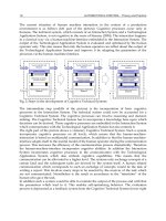
These two dilemmas span the so called polylemma of production technology (Fig. 1)
(Brecher et al, 2007). The reduction of these dilemmas is the main aim of the cluster of
excellence "Integrative Production Technology for High-Wage Countries" of the RWTH
Aachen University. The research vision is the production of a great variety of products in
2
AUTOMATION&CONTROL-TheoryandPractice14
small batch sizes with costs competitive to mass production under the full exploitation of
the respective benefits of value orientation and planning orientation.
To reach the vision four core research areas were identified. These areas are “Individualized
Production Systems”, “Virtual Production Systems”, “Hybrid Production Systems” and
“Self-optimizing Production Systems”. Self-optimizing production systems try to realize
value orientated approaches with an increase in the planning efficiency by reusing gained
knowledge on new production conditions.
The research hypothesis is that only technical systems which incorporate cognitive
capabilities are capable of showing self-optimizing behavior (Heide 2006). In addition to
that these Cognitive Technical Systems can reduce the planning efforts required to adapt to
changes in the process chain (Brecher et al. 2007). In this chapter a software architecture for
such a Cognitive Technical System will be described and a use case in the context of
assembly processes will be presented. Section 2 will deal with the definition of the terms
“Self optimization”, “Cognition” and “Cognitive Technical System”. Section 3 deals with
related work in the context of Cognitive Technical Systems and the involved software
architectures. The fourth section describes an excerpt of the functional as well as the non-
functional requirements for a Cognitive Technical System. Afterwards the software
architecture will be presented. The sixth section will introduce an assembly use case and the
chapter closes with a final conclusion in section 7.
2020
2006
dilemma
reduced
dilemmas
timeline
scale
scope
planning-
orientation
value-
orientation
resolution of the
polylemma of
production
20202020
20062006
dilemmadilemma
reduced
dilemmas
reduced
dilemmas
timeline
scale
scope
scale
scope
planning-
orientation
value-
orientation
planning-
orientation
value-
orientation
resolution of the
polylemma of
production
resolution of the
polylemma of
production
Fig. 1. Polylemma of Production Technology
2. Definition of Terms
2.1 Self-Optimization
Self-optimization in the context of artificial systems includes three joint actions. At first the
current situation has to be analyzed and in a second step the objectives have to be
determined. These objectives can be contradictive. In this case a tradeoff between the
objectives has to be done by the system. The third step is the adaption of the system
behavior. A system can be accounted for a self-optimizing system if it is capable to analyze
and detect relevant modifications of the environment or the system itself, to endogenously
modify its objectives in response to changing influence on the technical system from its
surroundings, the user, or the system itself, and to autonomously adapt its behavior by
means of parameter changes or structure changes to achieve its objectives (Gausemeier
2008). To adapt itself, the system has to incorporate cognitive abilities to be able to analyze
the current situation and adjust system behavior accordingly.
2.2 Cognition
Currently, the term “Cognition” is most often thought of in a human centered way, and is
not well defined in psychology, philosophy and cognitive science. In psychology Matlin
(2005) defines cognition in the context of humans as the “acquisition, storage, usage and
transformation of knowledge”. This involves many different processes. Zimbardo (2005)
accounts, among others, “perception, reasoning, remembering, thinking decision-making
and learning” as essential processes involved in cognition. These definitions cannot be easily
transferred to artificial systems. A first approach to the definition of “Cognition” in the
context of artificial systems is given in Strasser (2004). She based her definition on Strube
(1998):
“Cognition as a relatively recent development of evolution, provides adaptive (and hence,
indirect) coupling between the sensory and motor sides of an organism. This adaptive,
indirect coupling provides for the ability to learn (as demonstrated by conditioning, a
procedure that in its simplest variant works even in flatworms), and in higher organisms,
the ability to deliberate”.
Strasser develops from this the definition that a system, either technical or biological, has to
incorporate this flexible connectivity between input and output which implies the ability to
learn. Thereby the term learning is to be understood as the rudimentary ability to adapt the
output to the input to optimize the expected utility. For her, these are the essential
requirements a system has to incorporate to account for being cognitive.
This definition is to be considered when the term “Cognition” is used. It should be stated
that this definition is the lower bound for the usage of the term. Therefore this does not
imply that a system which can be accounted as “Cognitive” is able the incorporate human
level cognitive processes.
2.3 Cognitive Technical Systems
With the given definition for “Self-optimization” and “Cognition” the term “Cognitive
Technical System” can be defined. Also a description of the intermediate steps involved in
development towards a Cognitive Technical System able of incorporating cognitive
processes of a higher level can be given.
The definition used in the context of this chapter is that an artificial system, which
incorporates cognitive abilities and is able to adapt itself to different environmental changes,
can be accounted as Cognitive Technical System.
Fig. 2 shows the different steps towards a Cognitive Technical System capable of cognition
on a higher level. As cognitive processes of a higher level the communication in natural
language and adaption to the mental model of the operator can be named. Also more
sophisticated planning abilities in unstructured, partly observable and nondeterministic
environments can be accounted as cognitive processes on a higher level.
ASoftwareArchitectureforCognitiveTechnicalSystems
SuitableforanAssemblyTaskinaProductionEnvironment 15
small batch sizes with costs competitive to mass production under the full exploitation of
the respective benefits of value orientation and planning orientation.
To reach the vision four core research areas were identified. These areas are “Individualized
Production Systems”, “Virtual Production Systems”, “Hybrid Production Systems” and
“Self-optimizing Production Systems”. Self-optimizing production systems try to realize
value orientated approaches with an increase in the planning efficiency by reusing gained
knowledge on new production conditions.
The research hypothesis is that only technical systems which incorporate cognitive
capabilities are capable of showing self-optimizing behavior (Heide 2006). In addition to
that these Cognitive Technical Systems can reduce the planning efforts required to adapt to
changes in the process chain (Brecher et al. 2007). In this chapter a software architecture for
such a Cognitive Technical System will be described and a use case in the context of
assembly processes will be presented. Section 2 will deal with the definition of the terms
“Self optimization”, “Cognition” and “Cognitive Technical System”. Section 3 deals with
related work in the context of Cognitive Technical Systems and the involved software
architectures. The fourth section describes an excerpt of the functional as well as the non-
functional requirements for a Cognitive Technical System. Afterwards the software
architecture will be presented. The sixth section will introduce an assembly use case and the
chapter closes with a final conclusion in section 7.
2020
2006
dilemma
reduced
dilemmas
timeline
scale
scope
planning-
orientation
value-
orientation
resolution of the
polylemma of
production
20202020
20062006
dilemmadilemma
reduced
dilemmas
reduced
dilemmas
timeline
scale
scope
scale
scope
planning-
orientation
value-
orientation
planning-
orientation
value-
orientation
resolution of the
polylemma of
production
resolution of the
polylemma of
production
Fig. 1. Polylemma of Production Technology
2. Definition of Terms
2.1 Self-Optimization
Self-optimization in the context of artificial systems includes three joint actions. At first the
current situation has to be analyzed and in a second step the objectives have to be
determined. These objectives can be contradictive. In this case a tradeoff between the
objectives has to be done by the system. The third step is the adaption of the system
behavior. A system can be accounted for a self-optimizing system if it is capable to analyze
and detect relevant modifications of the environment or the system itself, to endogenously
modify its objectives in response to changing influence on the technical system from its
surroundings, the user, or the system itself, and to autonomously adapt its behavior by
means of parameter changes or structure changes to achieve its objectives (Gausemeier
2008). To adapt itself, the system has to incorporate cognitive abilities to be able to analyze
the current situation and adjust system behavior accordingly.
2.2 Cognition
Currently, the term “Cognition” is most often thought of in a human centered way, and is
not well defined in psychology, philosophy and cognitive science. In psychology Matlin
(2005) defines cognition in the context of humans as the “acquisition, storage, usage and
transformation of knowledge”. This involves many different processes. Zimbardo (2005)
accounts, among others, “perception, reasoning, remembering, thinking decision-making
and learning” as essential processes involved in cognition. These definitions cannot be easily
transferred to artificial systems. A first approach to the definition of “Cognition” in the
context of artificial systems is given in Strasser (2004). She based her definition on Strube
(1998):
“Cognition as a relatively recent development of evolution, provides adaptive (and hence,
indirect) coupling between the sensory and motor sides of an organism. This adaptive,
indirect coupling provides for the ability to learn (as demonstrated by conditioning, a
procedure that in its simplest variant works even in flatworms), and in higher organisms,
the ability to deliberate”.
Strasser develops from this the definition that a system, either technical or biological, has to
incorporate this flexible connectivity between input and output which implies the ability to
learn. Thereby the term learning is to be understood as the rudimentary ability to adapt the
output to the input to optimize the expected utility. For her, these are the essential
requirements a system has to incorporate to account for being cognitive.
This definition is to be considered when the term “Cognition” is used. It should be stated
that this definition is the lower bound for the usage of the term. Therefore this does not
imply that a system which can be accounted as “Cognitive” is able the incorporate human
level cognitive processes.
2.3 Cognitive Technical Systems
With the given definition for “Self-optimization” and “Cognition” the term “Cognitive
Technical System” can be defined. Also a description of the intermediate steps involved in
development towards a Cognitive Technical System able of incorporating cognitive
processes of a higher level can be given.
The definition used in the context of this chapter is that an artificial system, which
incorporates cognitive abilities and is able to adapt itself to different environmental changes,
can be accounted as Cognitive Technical System.
Fig. 2 shows the different steps towards a Cognitive Technical System capable of cognition
on a higher level. As cognitive processes of a higher level the communication in natural
language and adaption to the mental model of the operator can be named. Also more
sophisticated planning abilities in unstructured, partly observable and nondeterministic
environments can be accounted as cognitive processes on a higher level.