Macroeconomic theory and policy phần 9 ppsx
Bạn đang xem bản rút gọn của tài liệu. Xem và tải ngay bản đầy đủ của tài liệu tại đây (317.15 KB, 31 trang )
238 CHAPTER 11. INTERNATIONAL MONETARY SYSTEMS
went wrong—what happened was perfectly normal (which is to say that every-
thing is always going wrong in Argentina). Some people place the ‘blame’ on
the U.S. dollar, which strengthened relative to most currencies over the 1990s.
Since the Pe so was linked to the U.S. dollar, this had the effect of strengthening
the Peso as well, which evidently had the effect of making Argentina’s exports
uncompetitive on world mark ets. While there may be an element of truth to this
argumen t, one wonders how the U.S. economy managed to cope with the rising
value of its currency o ver the same period (in which the U.S. economy boomed).
Likewise, if the rising U.S. dollar made Argentine exports less competitive, what
prevented Argentine exporters from cutting their prices?
A more plausible explanation may be the following. First, the charter gov-
erning Argentina’s currency board did not require that Pesos be fully backed by
USD.Initially,asmuchasone-thirdofPesosissuedcouldbebackedbyArgen-
tine government bonds (which are simply claims to future Pesos). In the event
of a major speculative attack, t he currency board would not hav e enough USD
reserves to defend the exchange rate. Furthermore, it would likely have been
viewed as implausible to e xpect the Argentine government to tax its citizens t o
make up for any shortfall in reserves. Second, a combination of a weak economy
and liberal go vernment spending led to massive budget deficits in the late 1990s.
The climbing deficit led to an increase in devaluation concerns. According to
Spiegel (2002), roughly $20 billion in capital ‘fled’ the country in 2001.
5
Mark et
participan ts were clearly worried about the government’s ability to finance its
growing debt position without resorting to an inflation tax (Peso interest rates
climbed to between 40-60% at this time). In an attempt to stem the outflow
of capital, the government froze bank deposits, which precipitated a financial
crisis. Finally, the government simply gave up any pretense concerning its will-
ingness a nd/or ability to defend the exch ange rate. Of course, this simply served
to confirm market speculation.
At the end of the day, the currency board was simply not structured in a
way that would allow it to make good on its promise to redeem Pesos for USD
at par. In the absence of full credibility, a unilateral exchange rate peg is an
in viting target for currency speculators.
• Exercise 11.4. Explain why speculating against a currency that is
pegged unilaterally to a major currency like the USD is close to a ‘no-lose’
betting situation. Hint: explain what a speculator is likely to lose/gain
in either scenario: (a) a speculative attack fails to materialize; and (b) a
speculative attack that succeeds in devaluing the currency.
5
I presume what this means is that Argentines flocked to d i spose o f $ 2 0 billion in Peso-
denominated assets, using the proceeds to purchase foreign (primarily U.S.) assets.
11.2. NOMINAL EXCHANGE RATE DETERMINATION: FREE MARKETS239
11.2.4 Currency Union
A currency union is very much like a multilateral fixed exchange rate regime.
That is, different monies with fixed nominal exchange rates essentially constitute
a single money. The only substantiv e difference is t hat in a currency union, t he
cont rol of the money supply is taken out of the hands of individual member
coun tries and relegated to a central authority. The central bank of the European
Currency Union (ECU), for example, is located in Frankfurt, Germany, and is
called the European Central Bank (ECB). The ECB is governed by a board of
directors, headed by a president and consisting of the board of directors and
representatives of other central banks in the ECU. These other central banks
now behave more like the regional offices of the Federal Reserve system in the
United States (i.e., they no longer exert independent influence on domestic
monetary policy).
Having a centralized monetary authority is a good way to mitigate the lack of
coordination in domestic monetary policies that may poten tially afflict a m ulti-
lateral fixed exchange rate system. However, as the recent European experience
reveals, such a system is not free of political pressure. In particular, ECB mem-
bers often feel that the central authority neglects the ‘special’ concerns of their
respective coun tries. There is also the issue of how much seigniorage revenue
to collect and distribute among member states. The governments of member
coun tries may have an incentive to issue large amounts of nominal go vernment
debt and then lobby the ECB for high inflation to reduce the domestic tax
burden (spreading the tax burden across member countries). The success of a
currency union depends largely on the ability of the central authority to deal
with a variety of competing political interests. This is wh y a currency union
within a country is likely to be more successful than a currency union consisting
of different nations (the di fference, however, is only a matter of degree).
11.2.5 Dollarization
One way to eliminate nominal exchange rate risk that may exist with a major
trading partner is to simply adopt the currency of your partner. As mentioned
earlier, this is a policy that has been adopted by Panama, which has adopted
the U.S. dollar as its primary medium of exchange. Following the long slide in
the value of the Canadian dollar since the mid 1970s (see Figure 11.1), many
economists were a dvocating that Canada should adopt a similar policy.
One of t he obvious implications of adopting the currency of foreign country
is that the domestic country loses all control of its monetary policy. Depending
on circumstances, this may be viewed as either a good or bad thing. It is
likely a good thing if the government of the domestic country cannot be trusted
to maintain a ‘sound’ monetary policy. Any loss in s eigniorage revenue may be
more than offset by the gains associated with a stable currency and no exchange
rate risk. On the other hand, should the foreign government fi nd itself in a
240 CHAPTER 11. INTERNATIONAL MONETARY SYSTEMS
fiscal crisis, the value of the foreign currency may fall precipitously through an
unexpected inflation. In such an event, the domestic country would in effect
be helping the foreign government resolve its fiscal crisis (through an inflation
tax).
• Exercise 11.5. If the Argentine government had simply dollarized instead
of erecting a currency board, would a financial crisis have been averted?
Discuss.
11.3 Nominal Exc hange Rate Determination:
Legal Restrictions
The previous section described a world in which individuals are free to trade
in ternationally and free to hold different types of fiat monies. Since fiat money
is an intrinsically useless object, one fiat money is as good as any other fiat
money; i.e., in such world, different fiat monies are likely to be viewed as perfect
substitutes for each other. But if this is true, then there are no market forces
that pin down a unique exchange rate system between different fiat monies:
the nominal exchange rate is indeterminate. This indeterminacy problem can
be resolved only by government policy; i.e., via membership in a multilateral
exchange arrangement, or via the adoption of a c ommon currency.
The world so described appears to ring true along many dimensions. In par-
ticular, it seems capable of explaining why market-determined exchange rates
appear to display ‘excessive’ volatilit y. And it also explains why governments
are often eager to enter into multilateral fixed exchange rate arrangements. But
this view of the world is perhaps too extreme. In particular, if world currencies
are indeed perfect substitutes, then one would expect the currencies of differ-
ent coun tries to circulate widely within national borders. Casual observations
suggests, however, that national borders do, in large measure, determine cur-
rency usage. Furthermore, it is difficult (although, not impossible) to reconcile
the indeterminacy proposition with many historical episodes in which exchange
rates have floated with relative stability (see, for example, the behavior of the
Canada-U.S. exchange rate in the 1950s in Figure 11.1).
One element of reality that is missing from the model developed above is the
absence of legal restrictions on money holdings. These types of legal restrictions
are called foreign currency controls (FCC s). Foreign currency controls c ome in
a variety of guises. For example, chartered banks are usually required to hold
reserves of currency consisting primarily of domestic money or a restricted from
offering deposits denominated in foreign c urrencies.
6
Many countries have ‘cap-
ital controls’ in place that restrict domestic agents from undertaking capital
account transactions with foreign agents in an attempt to keep trade ‘balanced’
6
In the late 1970s, the Bank of America wanted to offer deposits denominated in Japanese
yen, but was officially discoura ged from doing so.
11.3. NOMINAL EXCHANGE RATE DETERMINATION: LEGAL RESTRI CTIONS241
(i.e., to reduce a growing current account deficit). An example of such a capital
con trol is a restriction on the ownership of assets not located in the country of
residence. In some countries, more Draconian measures are imposed; e.g., legal
restrictions are imposed that prohibit domestic residents from holding any for-
eign money whatsoever. Such legal restrictions, whether current or anticipated,
have the effect of generating a well-defined demand for individual currencies. If
the demands for individual currencies become well-defined in this manner, then
nominal exchange rate indeterminacy may disappear.
To see how this might work, let us consider an example that constitutes
the opposite extreme of the model studied above. Let us again consider two
coun tries, labelled a and b. It will be helpful to generalize the analysis here to
consider differen t population growth rates n
i
and different money supply growth
rates μ
i
for i = a, b.
Now, imagine that the governments in each country impose foreign currency
con t rols. Assume that this legal restriction does not prohibit international trade
(so that the young in one coun try may still sell output to the old of the other
coun try). But the legal restriction prohibits young individuals from carrying
foreign currency from one period to the next (i.e., domestic agents can only
save by accumulating domestic currency). In this case, if a young agent from
coun t ry a meets a n old agent from country b, the young agent may ‘export’
output to country b in exchange for foreign currency. But the FCC restriction
requires that the young agent in possession of the foreign currency dispose of
it within the period on the foreign exchange market (in exchange for domestic
currency).
The effect of these FCCs is to create two separate money markets: one for
currency a and one for currency b. In other words, each country now has its
own money supply and demand that independently determine the value of its
fiat money; i.e.,
M
a
t
= p
a
t
N
a
t
y;
M
b
t
= p
b
t
N
b
t
y.
With domestic price-levels determined in this way, the equilibrium exchange is
determined (by the LOP) as:
e
t
=
p
a
t
p
b
t
=
M
a
t
M
b
t
N
b
t
N
b
t
. (11.5)
The equilibrium inflation rate in each country (the inverse of the rate of return
on fiat money) is now determined entirely by domestic considerations; i.e.,
Π
a
=
μ
a
n
a
and Π
b
=
μ
b
n
b
.
From this, it follows that the time-path of the equilibrium exchange rate must
follow:
e
t+1
e
t
=
Π
a
Π
b
=
μ
a
μ
b
n
b
n
a
. (11.6)
242 CHAPTER 11. INTERNATIONAL MONETARY SYSTEMS
Thus, in the presence of such legal restrictions, the theory predicts that if
exchange rates are allowed to float, they will be determined by the relative
supplies and demands for each currency. Equation (11.5) tells us that, holding
all else constant, an increase in the supply of coun try a money will lead to a
depreciation in the exchange rate (i.e., e
t
, which measures the value of country b
money in units of country a money, rises). Equation (11.6) tells us that, holding
all else c onstant, an increase in the growth rate of country a money will cause it
to appreciate in value at a slower rate (and possibly depreciate, if e
t+1
/e
t
< 1).
11.3.1 Fixing the Exc hange Rate Unilaterally
Under a system of foreign currency controls, a country can in principle fixthe
exchange rate by adopting a simple monetary policy. Equation (11.6) suggests
how this may be done. A fixedexchangerateimpliesthate
t+1
= e
t
. This implies
that country a could fix the exc h ange rate simply by setting its monetary policy
to satisfy:
μ
a
=
n
b
n
a
μ
b
.
Essentially, this policy suggests that country a monetary policy should follow
country b monetary policy. In other words, this model suggests that a country
can choose either to fix the exchange rate or to pursue an independent monetary,
but not both simultaneously.
11.4 Summ ary
Because foreign exchange markets deal with the exchange of intrinsically useless
objects (fiat currencies), there is little reason to expect a free market in interna-
tional monies to function in any well-behaved manner. In the absence of legal
restrictions, or other frictions, one fiat object has the same intrinsic value as any
other fiat object (zero). Free markets are good at pricing objects with intrinsic
value; there is no ob v ious wa y to price one fiat object relative to another. It is
toomuchtoaskmarketstodotheimpossible.
If governments insist on monopolizing small paper note issue with fiat money,
how should international exc hange markets be organized? One possible answer
to this question is to be found in the way nations organize their internal money
markets. Most nations delegate the creation of fiat money to a centralized
institution (like a central bank). In particular, cities, provinces and states within
a n ation are not free to pursue distinct seigniorage policies. The d ifferen t monies
that circulate within a nation trade at fixed exchange rates (creating different
denominations) that are determined by the monetary authority. By and large,
this type of system appears to work t olerably well (most of the time) in a
relatively politically integrated structure like a nation.
11.4. SUMMARY 243
Does the same logic extend to the case of a world economy? Imagine a
world with a single currency. People travelling to foreign countries would never
have to first visit the foreign exchange booth at the airport. Firms engaged in
international trade could quote their prices (and accept payment) in terms of a
single currency. No one would ever have to worry about foreign exchange risk.
Such a world is theoretically possible. But such an arrangement would have
to overcome several severe political obstacles. First, a single world currency
would require that nations surrender their sovereignty over monetary policy
to some trusted international institution. (Given the dysfunctional nature of
the U.N. and the IMF, one may legitimately question the feasibility of this
requirement alone). This centralized authority would have to settle on a ‘one-
size-fits-all’ monetary policy and deal with the politically delicate question of
how to distribute seigniorage reven u e ‘fairly.’ Given that there are significant
differences in the extent to whic h international governments rely on seigniorage
revenue, reaching a consensus on this matter seems highly unlikely.
If a single world currency is politically infeasible, a close ‘next-best’ alter-
native would be a multilateral fixed exchange rate arrangement, like Bretton-
Woods (sans foreign currency con trols). Under this scenario, different cur-
rencies function as different denominations of the w orld money supply, freely
traded everywhere. Such a regime requires a high degree of coordination among
national monetary policies in order to prevent speculative attacks. More im-
portantly, it requires significant restraint on the part of national treasuries from
pressuring the local monetary authorities into ‘monetizing’ local government
debt. Under suc h a system, the temptation to export inflation to other coun-
tries may prove to be politically irresistible. This type of political pressure is
likely behind t he collapse of every international fixed exchange rate system ever
devised (including Bretton-Woods).
If common currency and mu ltilateral exchange rate arrangements are both
ruled out, then another alternative would be to impose foreign currency con trols
and allow the market to determine the exchange rate. But while foreign cur-
rency c ontrols eliminate the speculative dimension of exchange rate fluctuations,
exchange rates may still fluctuate owing to changes in marke t fundamen tals. A
gove rnment could, in principle, try to fix the exchange rate in this case, but
doingsowouldentailalossinsovereignty over the conduct of domestic mone-
tary policy. In any case, the imposition of legal restrictions on foreign currency
holdings is not without cost, since they hamper the conduct of international
trade (e.g., individuals are forced to make currency conversions that they would
otherwise prefer not to make).
A more dramatic policy ma y entail a return to the past, where governments
issued monetary instrument s that were backed by gold. In general, governments
might also issue money that is backed by other real assets (like domestic real
estate). Under this scenario, government money would presumably trade much
like any private security. The value o f government money wo uld depend on
both the value of the underlying asset backing the money and the government’s
244 CHAPTER 11. INTERNATIONAL MONETARY SYSTEMS
willingness and/or abilit y to make good on its promises. The relative price of
national monies would then depend on the market’s perception of the relative
credibility of competing governments. Governments typically do not like to issue
money backed in this manner, since it restricts their ability to extract seigniorage
revenue and otherwise conduct monetary policy in a ‘flexible’ manner.
But perhaps the ultimate solution may entail removing the governmen t
monopoly on paper money. By many accounts, historical episodes i n which pri-
vate banks issued ( fully-backed) money appeared to work reasonably well (e.g.,
the so-called U.S. ‘free-banking’ era of 1836-63). Despite problems of counter-
feiting (which are ob viously present with government paper as well) and despite
the coexistence of hundreds of different bank monies, these monies generally
traded more often than not at relatively stable fixed exchange rates.
7
Such a
regime, however, severely limits the ability of governments to collect seigniorage
reven u e. It is no coincidence that the U.S. ‘free-banking’ system was legislated
out of existence during a period of severe fiscal crisis (the U.S. civil war).
So there y ou have it. G iven the political landscape, it appears that no
monetary system is perfect. Each system entails a particular set of costs and
benefits that continue to be debated to this day.
11.5 R eferences
1. Champ, Bruce and Scott Freeman (2001). Modeling Monetary Economies,
2nd Edition, Cambridge University Press, Cambridge, U.K.
2. King, Robert, Neil Wallace, and Warren E. Weber (1992). “Nonfunda-
men t al Uncertainty and Exchange Rates,” Journal of International Ec o-
nomics, 32: 83—108.
3. Manueli, Rodolfo E. and James P eck (1990). “Exchange Rate Volatility
in an Equilibrium Asset Pricing M odel,” International Economic Review,
31(3): 559—574.
4. Roubini, Nouriel, Giancarlo Corsetti, and Paolo A. Pesenti (1998). “Paper
Tigers? A Model of the Asian Crisis,” Manuscript.
5. Spiegel, Mark (2002). “Argentina’s Currency Crisis: Lessons for Asia,”
www.frbsf.org/ publications/ economics/ letter/ 2002/ el2002-25.h tml
7
The episodes in which some banknotes traded at heavy discount were often directly re-
lated to state-specific fiscal crises and legal restrictions that forced state banks to hold large
quantities of state bon ds.
11.A. NOMINAL EXCHANGE RATE I NDETERMINACY AND SUNSPOTS245
11.A N om inal Exchange Rate Indeterminacy and
Sunspots
The indeterminacy of nominal exchange rates opens the door for multiple ratio-
nal expectations equilibria (self-fulfilling prophesies). This appendix formalizes
the restrictions placed on exchange rate behavior implied by our model; see also
Man u elli and Peck (1990).
Consider two countries a and b as described in the text. Individuals have
preferences given by E
t
u(c
2
(t +1)), where E
t
denotes an expectations operator.
Note that there is no fundamental risk in this economy. But there may be
nonfundamental risk owing to fluctuations in the exchange rate.
Let R
i
t+1
denote the (gross) rate of return on currency i = a, b (i.e., the
in verse of the inflation rate). Let q
i
t
denote the real money balances held of
currency i by an individual. Then an individual faces the following set of budget
constraints:
q
a
t
+ q
b
t
= y;
c
2
(t +1)=R
a
t+1
q
a
t
+ R
b
t+1
q
b
t
.
Substitute these constraints into the utility function. The individual’s choice
problem can then be stated as:
max
q
a
t
E
t
u
¡£
R
a
t+1
− R
b
t+1
¤
q
a
t
+ R
b
t+1
y
¢
.
A necessary (and sufficient) condition for an optimal choice of q
a
t
is giv en by:
E
t
£
R
a
t+1
− R
b
t+1
¤
u
0
(c
2
(t +1))=0.
Since the marginal utility of consumption is assumed to be positive, the condi-
tion above implies:
E
t
£
R
a
t+1
− R
b
t+1
¤
=0.
Let e
t
= p
a
t
/p
b
t
denote the nominal exchange rate. Then R
a
t+1
= p
a
t
/p
a
t+1
and R
b
t+1
= p
b
t
/p
b
t+1
. Hence, (e
t+1
/e
t
)=R
b
t+1
/R
a
t+1
or R
b
t+1
=(e
t+1
/e
t
)R
a
t+1
.
Substitute this latter condition into the previous equation, so that:
E
t
∙
1 −
µ
e
t+1
e
t
¶¸
R
a
t+1
=0.
Since R
a
t+1
> 0, this condition implies:
E
t
e
t+1
= e
t
.
This condition exhausts the restrictions placed on exchange rate behavior by
the theory. What the condition tells us is that the nominal exchange rate can
246 CHAPTER 11. INTERNATIONAL MONETARY SYSTEMS
be stochastic, but that the stochastic process must f ollow a Martingale.Inother
words, the best forecast for the future exchange rate e
t+1
is given by the current
(indeterminate) exchange rate e
t
. A special case is given by a deterministic
exchange rate; i.e., e
t+1
= e
t
. But many other outcomes are possible so that
the equilibrium exchange rate may fluctuate even in the absence of an y intrinsic
uncertain ty (i.e., no fundamental risk).
Note that, in equilibrium, q
a
t
and q
b
t
represent the average real money hold-
ings of individuals. These demands can fluctuate with the appearance of ‘sunspots.’
For example, if individuals (for some unexplained reason) feel like ‘dumping’
currency a, then q
a
t
will fall. Of course, since q
a
t
+ q
b
t
= y, such behavior im-
plies a corresponding increase in the demand for currency b. If individuals are
risk-averse (i.e., if u
00
< 0), then individuals would want to hedge themselves
against any risk induced by sunspot movemen ts in the exchange rate. One wa y
to do this is for all individuals to hold the average quantities q
a
t
and q
b
t
in their
portfolios. In this way, any depreciation in currency a is exactly offset by an
appreciation in currency b. However, if individuals find it costly to hedge in
this manner, then sunspot uncertainty will induce ‘unnecessary’ variability in
individual consumptions, leading to a reduction in economic welfare.
11.B. INTERNATIONAL CURRENCY TRADERS 247
11.B International Currency Traders
In the model of exchange rate indeterminacy developed in the text, it was as-
sumed that all individuals view different fiatcurrenciesasperfectsubstitutes.
In fact, all that is required for the indeterminacy result is that some group of
individuals view fiat currencies as perfect substitutes. In reality, this some group
of individuals can be thought of as large multinational firms that readily hold
assets denominated in either USD, Euros, or Yen (for example). In this case,
indeterminacy will prevail even if the domestic residents of (say) the United
States and Japan each prefer (or are forced by legal restriction) to hold assets
denominated in their national currency.
This idea has been formalized by King, Wallace and Weber (1992). To see
how this might w ork, consider extending our model to include three t ypes of
individuals A, B, and C,witheachtypeconsistingofafixed population N.
Think of t ype A individuals as Americans living in the U.S. (country a) and
type B individuals as Japanese living in Japan (country b).TypeC individuals
are ‘international’ citizens living in some other location (perhaps a remote island
in the Bahamas).
Assume that foreign currency controls force domestic residents to hold do-
mestic currency only. International citizens, however, are free to hold either
currency. Let q
i
t
denote the real money balances held by international citizens
intheformofi = a, b currency. Note that q
a
+ q
b
= y. Then the money-market
clearing conditions are given by:
M
a
= p
a
t
N(y + q
a
t
);
M
b
= p
b
t
N(y + q
b
t
).
The nominal exchange rate in this case is given by:
e
t
=
p
a
t
p
b
t
=
M
a
M
b
µ
y + q
b
t
y + q
a
t
=
M
a
M
b
µ
2y − q
a
t
y + q
a
t
.
This condition constitutes o ne equation in the two unknowns: e
t
and q
a
t
. Hence,
the exchange rate is indeterminate and may therefore fluctuate solely on the
‘whim’ of international currency traders (i.e., via their ch oice of q
a
t
). If interna-
tional currency traders are well-hedged (or if they are risk-neutral), exchange
rate volatility does not matter to them. But an y exchange rate volatilit y will
be welfare-reducing for the domestic residents of countries a and b.
248 CHAPTER 11. INTERNATIONAL MONETARY SYSTEMS
11.C The Asian Financial Crisis
Perhaps you’ve heard of the so-called Asian Tigers. This term was originally
applied to the economies of Hong Kong, South Korea, Singapore and Taiwan,
all of which displayed dramatic rates of economic growth from the early 1960s
to the 1990s. In the 1990s, other southeast Asian economies began to grow very
rapidly as well; in particular, Thailand, Malaysia, Indonesia and the Philippines.
These ‘emerging markets’ were subsequently added to the list of Asian Tiger
economies. In 1997, this impressive growth performance came to a sudden end
in what has subsequently been called the Asian Financial Crisis. What was this
all about?
Throughout the early 1990s, many small southeast Asian economies at-
tracted huge amounts of foreign capital, leading to huge net capital inflows
or, equivalently, to huge curren t account deficits. In other words, these Asian
economies were borrowing resources from the rest of the world. Most of these
resources were used to finance domestic capital expenditure. As we learned in
Chapters 4 and 6, a growing current accoun t deficit may signal the strength of
an economy’s future prospects. Foreign investors were forecasting high future
returns on the capital being constructed in this part of the world. This ‘opti-
mism’ is what fuelled much of the growth domestic capital expenditure, capital
inflows, and general growth in these economies. Evidently, this optimistic out-
look turned out (after the fact) to be misplaced.
What went wrong? One possible is that nothing went ‘wrong’ necessarily.
After all, rational forecasts can (and often do) turn out to be incorrect (after
the f act). Perhaps what happened was a growing realization among foreign
in ve stors that the high returns they were expecting were not likely to be realized.
Investors who realized this early on pulled out (liquidating their foreign asset
holdings). As this realization spread throughout the world, the initial trickle in
capital outflows exploded into a flood. Things like this happen in the process
of economic development.
Of course, there are those who claim that the ‘optimism’ displayed by the
parties involved was ‘excessive’ or ‘speculative;’ and that these types of booms
and crashes are what one should expect from a free market. There is another
view, however, that directs the blame toward domestic government policies; e.g.,
see (Roubini, Corsetti and Pesenti, 1998). For example, if a government stands
ready to bailout domestic losers (bad capital projects), then ‘overinv estment’
may be the result as private investors natural downplay the downside risk in
any capital investment. To the extent that foreign creditors are willing to lend
to domestic agents against future bail-out revenue from the government, unprof-
itable projects and cash shortfalls are refinanced through external borrowing.
While public deficits need not be high before a crisis, the eventual refusal of
foreign creditors to refinance the country’s cumulative losses forces the govern-
men t to step in and guarantee the outstanding stock of external liabilities. To
satisfy solvency, th e government must then undertake appropriate domestic fis-
11.C. THE ASIAN FINANCIAL CRISIS 249
cal reforms, possibly involving recourse to seigniorage reve nues. Expectations
of inflationary financing thus cause a collapse of the currency and anticipate the
event of a financial crisis.
There is also evidence that government corruption may have played a sig-
nificant role. For example, a domestic government may borrow money from
foreigners with the stated intent of constructing domestic capital infrastruc-
ture. But a significant fraction of these resources may simply be ‘consumed’
by government officials (and their friends). For example, in 2001 Prime Min-
ister Thaksin (of Thailand) was indicted for concealing huge assets when he
was Deputy Prime Minister in 1997. Evidently, Mr. Thaksin did not dispute
the charge. Instead, he said that the tax rules and regulations were ‘confusing’
and that he made an ‘honest mistake’ in concealing millions of dollars assets,
manipulating stocks and evading taxes.
8
As we saw during the recen t Enron
scandal, the market reacts quic kly and ruthlessly when it gets a whiff of financial
shenanigans.
9
The Asian crisis began in 1997 with a huge speculative attack on the Thai
currency (called the Baht). Prior to 1997, the Thai government had unilater-
ally pegged their currency at around 25 Baht per USD. Many commentators
have blamed this speculative attack for precipitating the Asian crisis. A more
plausible explanation, however, is that the speculative attack was more of a
symptom than a cause of the crisis (which was more deeply rooted in the nature
of go ve rnment policy).
Thai Baht per USD
8
See: www.pacom.mil/ publications/ apeu02/ 24Thailand11f.doc.
9
For m ore on the Enron fiasco, see: www.washingtonpost.com/ wp-dyn/ business/ sp e-
cials/ energy/ enron/
250 CHAPTER 11. INTERNATIONAL MONETARY SYSTEMS
In any case, financial crisis or not, our theory suggests that the Thai gov-
ernment could have maintained its fixed exchange rate policy and prevented
a speculative attack on its currency if it had either: (1) maintained sufficient
USD reserves; or (2) been willing to tax its citizens to raise the necessary USD
reserves. Evidently, as the Thai economy showed signs of weakening in 1997,
currency speculators believed that neither o f these conditions held (and in fact,
they did not).
Would the crisis in Thailand have been averted if the government had main-
tained a stable exchange rate? It is highly doubtful that this would have been
the case. If the crisis was indeed rooted in the fact that many bad investments
were made (the result of either bad decisions or corruption), then the contrac-
tion in capital spending (and the corresponding capital outflows) would have
occurredwhethertheexchangeratewasfixed or not. But this is just one man’s
opinion.
Chapter 12
M oney, Capital and
Banking
12.1 In troduction
An almost universal feature of most economies is the coexistence of ‘base’ and
‘broad’ money instruments. In modern economies, the monetary base consists
of small denomination governmen t paper notes, while broad money consists
of electronic book-entry credits created by the banking system redeemable in
base money. In earlier historical episodes, the monetary base often consisted
of specie (gold or silver coins) with broad money consisting of privately-issued
banknotes redeemable in base money. In this chapter, we consider a set of simple
models designed to help us think about the determinants of such monetary
arrangemen ts.
12.2 A Model with Money and Capital
Consider a model economy consisting of overlapping generations of individuals
that live for two periods. The population of young individuals at date t ≥
1 is given by N
t
and the population gro w s at some exogenous rate n>0;
i.e., N
t
= nN
t−1
. There is also a population N
0
of individuals we call the
‘initial old’ (who live for one period only). To simplify, we focus on stationary
allocations and assume that individuals care only about consumption when old;
i.e., U(c
1
,c
2
)=c
2
.
As before, assume that each young person has an endowment y>0. Unlike
our earlier OLG model, however, assume that output can be stored over time
in the form of capital. In particular, k units of capital expenditure at date t
251
252 CHAPTER 12. MONEY, CAPITAL AND BANKING
yields zf(k) units of output at date t +1, where f is increasing and strictly
concave in k. Assume (for simplicity) that capital depreciates fully after its use
in production. Note t hat zf
0
(k) represents the marginal product of (future)
capital. From Chapter 6, we know that zf
0
(k) will (in equilibrium) be equal to
the (gross) real rate of interest.
It will be useful to consider first how this economy functions without money.
The equilibrium, in this case, is simple to describe. In particular, since young
individuals care o nly for future consumption, they will sa ve their entire endow-
men t in the form of capital spending; i.e., k = y. In this way, the young end up
consuming c
2
= zf(y). The economy’s GDP at any given date t is given b y:
Y
t
= N
t
y + N
t−1
zf(y).
Let us now introduce money into this economy. Assume that there is a
supply of fiat money M
t
that is initially (i.e., as of date 1) in the hands of
the initial old. The money supply grows at an exogenous rate μ ≥ 1 so that
M
t
= μM
t−1
. Assume that new money is used to finance governmen t purch ases.
Let Π denote the (gross) rate of inflation, so that Π
−1
represents the (gross)
real return on fiat money. From Chapter 10, we know that in an equilibrium
where fiat money is valued, its rate of equilibrium rate of return will be given
by Π
−1
= n/μ.
A young individual now faces a portfolio choice problem. That is, there are
now two ways in which to sav e for future consumption: money and capital.
Let q denote the real money balances acquired by a young individual (from the
existing old generation). The portfolio choice is restricted to satisfy q + k = y.
A simple no-arbitrage condition implies that both money and capital must earn
thesamerateofreturn(ifbothassetsaretobewillinglyheld). Therefore,the
equilibrium level of capital spending must satisfy:
zf
0
(k
∗
)=
n
μ
. (12.1)
This equilibrium is displayed in Figure 12.1.
12.2. A MODEL WITH MONEY AND CAPITAL 253
0
zf’(k)
n/m
k
Rates of
Return
k*
FIGURE 12.1
Coexistence of Money and Capital
y
zf’(y)
A
B
P oint A in Figure 12.1 displa ys the equilibrium without money. In this sce-
nario, the lev el of capital investment is ‘high’ so that the return to capital is
‘low’ (recall that we are assuming a diminishing marginal product of capital).
If n/μ > zf
0
(y), then young individuals are willing to divert some of their sav-
ings away from capital into money. As capital spending declines, the marginal
product of capital rises until the return on capital is equated to the return on
money (point B).
• Exercise 12.1. Consider Figure 12.1. Explain why the welfare of all
individuals (including the initial old) is higher at point B relative to point
A. Explain why this is so despite the fact that real GDP is lower at an
equilibrium associated with point B.
• Exercise 12.2. Use the model developed above to explain the likely
economic consequences of a decline in z. Hint: recall that z here has the
in terpretation of being the current period forecast of future productivity.
In particular, emphasize the likely impact of this ‘bad news’ shock on
capital spending, the demand for money, and future GDP.
254 CHAPTER 12. MONEY, CAPITAL AND BANKING
12.2.1 The Tobin Effect
Equation (12.1) suggests that while monetary policy may be neutral, it is un-
likely to be superneutral.
1
Consider, for example, an exogenous (permanent)
increase in the money growth rate μ. In this model, such a policy has the effect
of increasing the expected and actual rate of inflation. Since the real rate of
return on money is inversely related t o the inflation rate, the expected return on
money falls. If the return on money f alls, equation (12.1) suggests that individ-
uals will substitute out of money and into capital (i.e., rebalance their wealth
portfolios) to a point at which all assets again earn the same rate of return (see
also Figure 12.1). Since the real GDP in this economy is given by:
Y
t
= N
t
y + N
t−1
zf(k
t−1
),
it follows that such a ‘loosening’ of monetary policy has the effect of expanding
the future GDP (as the expansion in current capital spending adds to the future
capital stock). The substitution of private capital for fiat money in reaction to
an anticipated inflation is called the Tobin effect (Tobin, 1965).
The Tobin effect appears to present policymakers with a policy tool that
may be used to ‘stimulate’ the economy during a period of economic recession
or stagnation. In fact, some economists have adv ocated such a policy for Japan,
which struggled throughout the 1990s with low economic growth and low in-
flation(andevendeflation). In a deflationary environment, the rate of return
on money is high, making capital investment relatively unattractive. For this
reason, many people view deflation as undesirable leading them to advocate a
policy geared tow ard increasing t he inflation rate.
The l ogic underpinning the Tobin effect is compelling enough, but a few
cav eats are in order. First of a ll, it is important not to confuse GDP with
economic welfare. An inflation-induced expansion of the capital stock (and
GDP) in our model unambiguously reduces the welfare of all individuals. In
particular, a very high inflation would move the economy from point B to point
A in Figure 12.1 (see exercise 12.1). One can, in fact, show that the ‘optimal’
money growth rate in this model is zero (achiev ed by setting μ =1), which (for
n>1) implies that deflation is optimal.
2
There are also some practical difficulties a ssociated with exploiting the Tobin
effect in reality. T he first of these is that the stock of fiat money is typically
tiny relat ive to the size of the stock o f capital. Thus, while one may accept the
logic of the Tobin effect , one may legitimately question whether the effect can be
quantitatively important (probably not). The second problem is that while our
model features a clear link between money growth and inflation expectations,
1
That is, note that capital sp ending (and other real variables) do es not dep end on the
money stock M
t
; but does depend on the money growth rate μ.
2
Few p eople appear to take seriously the notion that defla t ion is op tima l. T h is vie w h a s
largely b een shap ed by the experience of the G reat Depression. H owever, there are many
(ear lie r) hi storica l ep is od e s in w h ich booms were ass oc ia t ed with de flations. These episodes
app ear to have b een erased from so ciety’s collective m emory bank.
12.3. BANKING 255
in reality this link appears to be not so tight. In Japan, for example, inflation
expectations appear to remain lo w even today despite several years of rapidly
growing government money and debt.
3
12 .3 B a nkin g
In the model developed above, fiat money and physical capital are viewed as
perfect substitutes; i.e., each asset serves the same purpose and earns the same
rate of return. In some sense, physical capital in this model is a type of ‘private
money’ that competes with government fiat money. In the model, this private
money can be thought of as privately-issued notes representing claims against
capital (e.g., corporate bonds). In equilibrium, individuals are indifferent be-
tween getting paid in government or private paper.
In reality, most privately-issued debt instruments are not widely used as a
means of payment. An important exception to this general rule are the liabilities
issued by banks; sometimes called demand-deposit liabilities. If you have a bank
account, then most your money (not wealth) is likely held in the form of this
‘bankmoney’ (electronic credits in a checkable account). Every time you use
y our debit card or write a check, you are in effect making a payment with
bankmoney (i.e., the banking system simply debits your account electronically
and makes corresponding credit entries to the accounts of merchants—no paper
money is involved in such transactions).
But we do n ot use bankmoney for all of our transactions. For some transac-
tions, we find it convenient to use government money (cash). Few of us actually
get paid in cash; our employers pay us in bankmoney (i.e., by writing a chec k or
making a direct transfer to our bank account). When we need cash, we can visit
a bank or ATM and mak e a withdrawal. Note that our bankmoney constitutes
a demandable liability of the bank. That is, w e can visit an ATM at any time
and demand the redemption of our bankmoney for cash (at par value).
Several questions may be popping to mind here. How are we to understand
the coexistence of fiat money and private money? Why is private money almost
always made redeemable on demand for cash (i.e., either government fiat or
historically in the form of specie)? Are banks free to ‘print’ all the bankmoney
they want? What is the function of banks—what do they do? Are they simply
repositories for cash, or do they serve some other function? What might happen
if all depositors wanted to withdraw cash from the banking system at the same
time? To help organize our thinking on these matters, let us develop a simple
model.
3
One p ossible explanation for th is is that the Japanese are expecting the government to
pay back the debt out of direct tax revenue instead of seigniorage.
256 CHAPTER 12. MONEY, CAPITAL AND BANKING
12.3.1 A Simple M odel
The formal model associated with this section can be found in Andolfatto (200*).
In what follows here, we will make do with an informal description. The econ-
omy is similar to that described above. Imagine, however, that individuals
populate two ‘spatially separated’ locations, labelled A and B. Each location
is identical in terms of population, technology and endowments. Assume that
individuals living in a location do not accept private liabilities issued by agents
living in the ‘foreign’ location. There are several ways in which to interpret
this restriction. One interpretation is that local residents do not trust ‘foreign’
paper, perhaps because it is difficult to detect coun terfeits (unlike locally issued
money or government cash). Another interpretation is that the two locations
are not connected electronically, so that debit card transactions are not feasible
for ‘tourists’ visiting the foreign location.
Young individuals have an endo wment y and have access to an investment
technology that tak es k units of output today and returns zk units of output in
the future; i.e., assume constant returns to scale so that f(k)=k. In this case,
the (gross) return to capital spending is given by z. Assume that z>nand that
μ =1(constant supply of fiat money). In this case, capital dominates money in
rate of return (as is typically the case in reality). But if capital (private money)
dominates fiat money, why is the latter held at all? In order to be valued, fiat
money cannot be a perfect substitute for capital—it needs to fulfill some other
purpose.
This other purpose is generated in the following way. Young individuals
must make a portfolio decision (money versus capital). Imagine that after this
decision is made, a fraction 0 <π<1 of young individuals at each location
are exogenously transported to the foreign location. Assume that they cannot
take their capital with them. They could try to take paper notes representing
claims to the capital they left behind, but by assumption, such claims are not
‘recognized’ in the ‘foreign’ location. How then are these ‘visiting’ individuals
to purchase the consumption they desire when old? One way would be to use
a payment instrument that is widely recognizable, like government fiat or gold.
In this s ense then, it is useful to think of π as an the probability of experiencing
an individual ‘liquidity’ shock (i.e., of encoun tering a situation where merchants
will only accept cash).
Since young individuals are uncertain about whether they will need cash in
a future transaction, they will want to hedge their bets (if they are risk-averse)
by holding some capital and some cash in their portfolio. Hedging in this w ay
is better than not hedging at all, but it is still inefficient. Since there is no
aggregate uncertainty, it would make sense for young individuals to pool their
risk. One way of doing this is through a bank that operates in the following
way .
Imagine that young individuals ‘deposit’ their endowment (real labor earn-
ings) with a bank. In return, the bank offers each depositor an interest-bearing
12.3. BANKING 257
accoun t that is redeemable (on demand) for government cash. If individuals do
not make an early withdrawal, they earn a real interest rate equal to z (and
consume locally). If they make an early withdrawal (because the experience the
liquidity shock), they earn a real return equal to n<z(and consume in the
foreign location).
A competitive bank would structure its balance sheet in the following way.
It would tak e the deposits made to the bank and use some of the deposits to
acquire cash (from the existing old agents). How much cash a bank should hold
in reserve depends on how much cash is forecasted to be withdra w n. In our
model, there is no aggregate uncertainty so that the bank can easily forecast
that a known fraction π of its depositors will want to make an early withdrawal.
Any resources that are not used up in the form of cash reserv es can then be used
to finance capital spending (e.g., making loans to entrepreneurs or acquiring the
capital directly). The bank can then use the return on its loan portfolio to pay
the interest its own liabilities (i.e., the interest on its deposit accounts).
A few observations are in order. First, note that the balance sheet of our
model bank resembles the balance sheet of real banks. That is, the asset side
consists of loans and cash reserves. The liability side consists of demandable
debt. This demandable debt earns a higher return than government cash and is
used widely as a form of payment. But not all places accept bankmoney (checks
or debit cards). For t his reason, banks stock their ATMs with g overnment cash
and allow their depositors to withdra w this cash on demand.
Second, note that banks are not free to create unbacked money (unlike the
gove rnment). A well-run bank will be ‘well-capitalized’ in the sense that it
should have assets of sufficient value to back up its outstanding liabilities. Note,
however, this does not mean a bank will hold all of its assets in the form of
gove rnment cash (which would correspond to a 100% reserve requirement). By
holding less than 100% reserves, banks are able to facilitate the financing of
productive capital projects (that might not o t herwise g et financed). Of course,
banks can be subject to fraudulent activity; for example, if a loans officer grants
a loan to a friend (who has no intention of repaying) and tries to pass it off
as an ‘investment.’ But fraud is illegal and is, in any case, not specifictothe
banking industry.
Finally, there is an issue of whether banks are in some sense ‘fragile’ financial
structures that may be subject to ‘bank runs’ (where everyone rushes to the bank
to withdraw cash). The reason people worry about this is owing to the structure
of a bank’s balance sheet. In particular, its assets are r elatively ‘long-term’ and
‘illiquid,’ while its liabilities constitute a form of very short-term debt (i.e.,
demandable debt). Of course, I argued above that this balance sheet structure
is no accident; i.e., this is the business of banking. But the question remains
as to whether such a structure is susceptible to collapse that is generated, for
example, by a self-fulfilling prophesy. What if, for example, everyone suddenly
perceives a bank to be insolvent. Then they will ‘run’ to the bank to withdraw
their cash. If everyone runs, there will not be e nough cash to satisfy depositors.
258 CHAPTER 12. MONEY, CAPITAL AND BANKING
The bank will then be forced to liquidate its assets quickly at firesale prices,
possibly rendering the bank insolv ent and confirming the initial expectation.
Certainly, there have been historical episodes that seem to fit the description
abo ve. It is not clear, however, whether such episodes were the product of
banking per se or of gov ernment restrictions on bank behavior. For example,
branch banking was for many years prohibited in the United States but not
in Canada, leading to thousands of smaller banks in the U.S. and only a few
larger banks in Canada. It is well-know n that many banks failed in the U.S.
during the Great Depression whereas none did in C anada. In another example,
man y of the state banks of the so-called U.S. ‘free-banking’ era were forced to
hold as assets state bonds of questionable quality. When state governments fell
into fiscal crisis, banks that held government bonds naturally did too. Both of
these examples are often cited as evidence of banking ‘instability.’ However, in
both cases, legal restrictions were in place that prevented banks from creating
a well-diversified asset portfolio.
12.3.2 Interpreting Money Supply Fluctuations
As I have remarked before, much of an econom y ’s money supply is in the form
of demand deposit liabil ities created by private banks. These liabilities are con-
vertible on demand (and at par) for go vernment cash. The fact that bankmoney
is convertible at par with government cash effectively fixes the nominal exchange
rate between bankmoney and fiat money. One popular definition of an econ-
omy’s total supply of money is therefore given by the sum of government cash
(in circulation) and the demandable liabilities created by chartered banks. This
definition of money is called M 1. Broader measures of money may include other
t y pes of private securities, including savings accounts, term deposits, money
market mu tual fund balances, and so on.
Most of the fluctuations in an economy’s money supply stems from fluctua-
tions in bankmoney, or the so-called ‘money-multiplier.’ The money multiplier
is defined as the total money supply divided by (essentially) the monetary base
(i.e., government cash). Fluctuations in the money multiplier (or broad money)
appear to be closely linked with fluctuations in real output. Changes in the
current money supply appear to be positively correlated with future changes
in real GDP. Why does the money supply vary in this manner? Does the ob-
served money-output correlation imply that a monetary authority stimulate the
economy with a surprise injection of cash?
To help address these questions, let us consider the model developed above
(and stated formally in the appendix). Assume that the stoc k of governmen t
money remains fixed at M. Let (q
∗
,k
∗
) denote the bank’s (or banking system’s)
optimal portfolio choice. Note that this choice will depend on the model’s
parameters. T he parameter I wish to emphasize here is z; i.e., the current
forecast of the future return to capital investment. Under a mild restriction on
preferences, the model implies that k
∗
is an increasing function of z. In other
12.3. BANKING 259
words, capital spending today responds positively to ‘news’ of a higher expected
return on capital (note that z also corresponds to the real rate of interest in this
economy). Since q + k = y, it follows that the demand for real money balances
is a decreasing function of z. In other words, news of a higher z leads market
participants (including banks) to substitute out of cash and into capital (banks
would accomplish this by extending more loans to finance capital spending).
Now imagine that the economy is continually hit by shocks that take the
form of changes in z. What are the economic implications of such disturbances
and, in particular, how do they affect the money supply?
Let us begin with the money-market clearing condition:
M
t
p
t
= N
t
q
t
.
For simplicity, let us hold the supply of fiat money and the population fixed.
Then the equilibrium price-level will satisfy:
p
∗
t
=
M
Nq
∗
t
. (12.2)
• Exercise 12.3. Imagine that the economy receives ‘news’ that leads
individuals to revise downward their forecast of z. What effect is such a
shoc k likely to have on the real interest rate and the price-level? Explain.
Now recall that the total money supply (M1
t
) is the sum cash and bankmoney.
The real value of a bank’s physical capital is given by Nk
∗
t
(assuming that it
has N depositors). The nominal value of this bankmoney is given by p
∗
t
Nk
∗
t
, so
that:
M1
t
= M + p
∗
t
Nk
∗
t
.
Substituting equation (12.2) into this latter expression, one can derive:
M1
t
= M +
M
Nq
∗
t
Nk
∗
t
; (12.3)
=
∙
1+
k
∗
t
q
∗
t
¸
M.
The term in the square brackets above is the money-mu ltiplier M1/M. Our
model suggests that the money multiplier is positively related to the ‘deposit-
to-currency’ ratio k/q.
Now consider the empirical observation that changes in the current money
supply M1
t
appear to be positively correlated with future changes in real GDP.
We can use the model developed here to interpret such a correlation. Suppose,
for example, that the economy is subject to ‘news’ shocks that lead people
to constantly revise their forecasts of z (the future return to current capital
spending). Consider, for example, a sudden increase in z. From our earlier
260 CHAPTER 12. MONEY, CAPITAL AND BANKING
discussion, such a shock should lead individuals (or banks acting on their behalf)
to substitute out of cash and into capital investment. In other words, k
∗
t
should
increase and q
∗
t
should decrease. From equation (12.3), we see this reaction
will lead to an increase in the money multiplier and hence to an increase in
M1
t
(even if M remains constant). Furthermore, the increase in current period
capital spending will translate (together with t he increase in z, if it materializes)
in to higher levels of future GDP.
Notice that while our model can replicate the observed money-output cor-
relation, the model suggests that it would be wrong to interpret the current
increase in M1
t
as having ‘caused’ the future increase in real GDP. In fact, the
direction of causality is reversed here; i.e., it is the increase in (forecasted) real
GDP that ‘causes’ an increase in the current money supply. This is an example
of what economists call ‘reverse causation,’ and serves as a useful warning for
us not to assume a direction of causality simply on the basis of an observ ed
correlation (e.g., we would not, for example, assert that Christmas shopping
‘causes’ Christmas, even though though early-December Christmas shopping is
positively correlated with the future arrival of Christmas).
12.4 Summary
To be written (chapter is incomplete).
12.5 R eferences
1. Andolfatto, David (2003). “Taking Intermediation Seriously: A Com-
men t ,” Journal of Money, Credit and Banking, 35(6-2): 1359—1366.
2. Tobin, James (1965). “Money and Economic Growth,” Econometrica, 33:
671—84.
Part III
Economic Growth and
Developmen t
261