Microeconomics principles and analysis phần 3 pptx

110 CHAPTER 5. THE CONSUMER AND THE MARKET
Figure 5.5: Consumption in the household-production model
j + 1 is
w
j
b
2j+1
 w
j+1
b
2j
w
j
b
1j+1
 w
j+1
b
1j
: (5.22)
We can think of this as ratio of notional prices 
1
=
2
. So it is clear that a simple
increase in the budget y (from a larger resource endowment) j ust “in‡ates”the
attainable set –look at the way each vertex (5.21) changes with y –without
altering the relative slopes of di¤erent parts of the frontier (5.22). However
changes in input prices or productivities will change the shape of the frontier.
As illustrated the household would consume at x


using a combination of
input (market good) 4 and input 5 to provide itself with output goods 1 and 2.
The household does not bother buying market good 3 because its market price
is too high. Now suppose something happens to reduce the price of market
good 3 – w
3
falls in (5.21) and (5.22). Clearly the frontier is deformed by
this – vertex 3 is shifted out along the ray through 0. Assume that R
3
= 0:
then, if the price of market good 3 falls only a little, nothing happens to the
household’s equilibrium;
10
the new frontier shifts slightly outwards at vertex 3
and the household carries on consuming at x

. But suppose the price w
3
falls a
lot, so that the vertex moves out as shown in in Figure 5.6. Note that techniques
4 and 5 have now both dropped out of consideration altogether and lie inside the
new frontier. Market good 3 has become so cheap as to render them ine¢ cient:
the consumer uses a combination of the now inexpensive market good 3 and
10
How wou ld this behaviour change if R
3
> 0?
5.4. HOUSEHOLD PRODUCTION 111
Figure 5.6: Market price change causes a switch
market good 6 in order to produce the desired consumption goods that yield

utility directly. The household’s new c onsu mption point is at x

.
The fact that some commodities are purchased by households n ot for direct
consumption but as inputs to produce other goods within the household enables
us to understand a number of phenomena that are di¢ cult to reconcile in the
simple consumer-choice model of section 4.5 (chapter 4):
 If m > n, some market goods may not be purchased. By contrast, in
the model of chapter 4, if all indi¤erence curves are strictly convex to the
origin, all go ods must be consumed in positive amounts.
 If the market price of a good falls, or indeed if there is a technical im-
provement in some input this may lead to no change in the consumer’s
equilibrium.
 Even though each x
i
may be a “normal”good, certain purchased market
goods may appear “inferior”if preferences are non-homothetic.
11
 The demand for inputs purchased in the market may exhibit jumps: as
the price of an input drops to a critical level we may get a sudden switch
from one facet to another in the optimal consumption plan.
11
Provide an intuitive argument why this may occur.
112 CHAPTER 5. THE CONSUMER AND THE MARKET
5.5 Aggregation over goods
If we were to try to use any of the consumer models in an empirical study we
would encounter a number of practical di¢ culties. If we want to capture the …ne
detail of consumer choice, distinguishing not just broad categories of consumer
expenditure (food, clothing, housing ) but individual product types within
those categories (olive oil, peanut oil) almost certainly th is would require that

a lot of components in the commodity vector will be zero. Zero quantities are
awkward for some versions of the consumer model, although they …t naturally
into the household production paradigm of section 5.4; they may raise prob-
lems in the speci…cation of an econometric model. Furthermore attempting to
implement the model on the kind of data that are likely to be available from
budget surveys may m ean that one has to deal with broad commodity categories
anyway.
This raises a number of deeper questions: How is n, the number of com-
modities determined? Should it be taken as a …xed number? What determines
the commodity boundaries?
These problems could be swept aside if we could be assured of some de-
gree of consistency between the model of consumer behaviour where a very …ne
distinction is made between commodity types and one that involves coarser
groupings. Fortunately we can appeal to a standard commonsense result (proof
is in Appendix C):
Theorem 5.1 (Composite commodity) The relative price of good 3 in terms
of good 2 always remains the same. Then maximising U(x
1
; x
2
; x
3
) subject to
p
1
x
1
+ p
2
x

2
+ p
3
x
3
 y is equivalent to maximising a function U(x
1
; x) subject
to p
1
x
1
+ px  y where p := p
2
+ p
3
, x := x
2
+ [1  ]x
3
,  := p
2
=p.
An extension of this result can be made from three to an arbitrary number of
commodities,
12
so e¤ectively resolving the p roblem of aggregation over groups
of goods. The implication of Theorem 5.1 is that if the relative prices of a group
of commodities remain unchanged we can treat this group as though it were a
single commodity.

The result is powerful, because in many cases it makes sense to simplify
an economic model from n commodities to two: theorem 5.1 shows that this
simpli…cation is legitimate, providing we are prepared to make the assumption
about relative prices.
5.6 Aggregation of consumers
Translating the elementary models of consumption to a real-world application
will almost certainly involve a second type of aggregation – over consumers.
We are not talking here about subsuming individuals into larger groups –such
as families, households, tribes – that might be considered to have their own
12
Provide a on e-line argument of why this can be done.
5.6. AGGREGATION OF CONSUMERS 113
coherent objectives.
13
We need to do something that is much more basic –
essentially we want to do the same kind of operation for consumers as we did for
…rms in section 3.2 of chapter 3. We will …nd that this can be largely interpreted
as treating the problem of analysing the behaviour of the mass of consumers as
though it were that of a “representative”consumer –representative of the mass
of consumers present in the market.
To address the problem of aggregating individual or household demands we
need to extend our notation a little. Write an h superscript for things that
pertain speci…cally to household h so:
 y
h
is the income of household h
 x
h
i
means the consumption by h of commodity i,

 D
hi
is the corresponding demand function.
We also write n
h
for the number of households.
The issues that we need to address are: (a) How is aggregate (market) de-
mand for commodity i related to the demand f or i by each individual household
h ? (b) What additional conditions, if any, need to be imposed on preferences
in order to get sensib le results from the aggregation? Let u s do this in three
steps.
Adding up the goods
Suppose we know exactly the amount that is being consumed by each household
of a particular good:
x
h
i
; h = 1; :::; n
h
: (5.23)
To get the total amount of i that is being consumed in the economy, it might
seem that we should just stick a summation sign in front of (5.23) so as to get
n
h
X
h=1
x
h
i
: (5.24)

But this step would involve introd ucing an important, and perhaps unwarranted,
assumption –that all goods are “rival” goods. By this we mean that that my
consumption of one more unit of good i means that there is one less unit of good
i for everyone else. We shall, for now, make this assumption; in fact we shall
go a stage further and assume that we are only dealing with pure private goods
–goods that are both rival and “excludable” in that it is possible to charge a
price for them in the market.
14
We shall have a lot more to say about rivalness
and excludability in chapters 9 onwards.
13
Is the re any sensible meaning to be given to aggregate preference or derings?
14
Can you think of a good or service that is not rival? One that is not excludable?
114 CHAPTER 5. THE CONSUMER AND THE MARKET
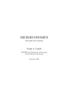
Figure 5.7: Aggregation of consumer demand
The representative consumer
If all goods are “private goods”then we get aggregate demand x
i
as a function of
p (the same price vector for everyone) simply by adding up individual demand
functions:
x
i
(p) :=
n
h
X
h=1
D

hi

p; y
h

(5.25)
The idea of equation (5.25) is depicted in the two-person case in Figure 5.7
and it seems that the elementary process is similar to that of aggregating the
supply of output by …rms, depicted in Figures 3.1 and 3.2. There are similar
caveats on aggregation and market equilibrium as for the …rm
15
–see pages 51
to 53 for a reminder –but in the case of aggregating over consumers there is a
more subtle problem.
Will the entity in (5.25) behave like a “proper” demand function? The
problem is that a demand function typically is de…ned on prices and some simple
measure of income –but clearly the right-hand side of (5.25) could be sensitive
to the distribution of income amongst households, not just its total. One way
of addressing this issue is to consider the problem as that of characterising the
behaviour of a representative consumer. This could be done by focusing on the
person with average income
16
y :=
1
n
h
n
h
X
h=1

y
h
15
Take the beer-and-cider example of Chapter 4’s note 9 (page 80). Show that my demand
for cider on a Friday night has a disco ntinuity. Suppose my tastes and income are typical for
everyone in London. Explain why London’s demand fo r cider on a Friday nigh t is e¤ectively
contin uous.
16
This is a very nar row de…nition of the “representative consumer” that makes the calcu-
lat ion ea sy: sug gest some alternat ive implementable de…nitions.
5.6. AGGREGATION OF CONSUMERS 115
Figure 5.8: Aggregable demand functions
and the average consumption of commodity i
x
i
:=
1
n
h
n
h
X
h=1
x
h
i
:
Then the key question to consider is whether it is possible to write the com-
modity demands for the person on average income as:
x

i
=

D
i
(p; y) (5.26)
where each

D
i
behaves like a conventional demand curve. If such a relationship
exists, then we may write:

D
i
(p; y) =
1
n
h
n
h
X
h=1
D
hi

p; y
h

(5.27)

If you were to pick some set of functions D
hi
out of the air –even though they
were valid demand functions for each individual household – they might well
not be capable of satisfying the aggregation criterion in (5.26) and (5.27) above.
In fact we can prove (see Appendix C)
Theorem 5.2 (Representative Consumer) Average demand in the market
can be written in the form (5.26) if and only if, for all prices and incomes,
individual demand functions have the form
D
hi

p; y
h

= a
h
i
(p) + y
h
b
i
(p) (5.28)
116 CHAPTER 5. THE CONSUMER AND THE MARKET
Figure 5.9: Odd things happen when Alf and Bill’s demands are combined
In other words aggregability across consumers imposes a stringent require-
ment on the ordinary demand curves for any one goo d i –for every household h
the so-called Engel curve for i (demand for i plotted against income) must have
the same slope (the number b
i

(p)). This is illustrated in Figure 5.8. Of course
imposing this requirement on the demand function also imposes a correspond-
ing condition on the class of utility functions that allow one to characterise the
behaviour of the market as though it were that of a representative consumer.
Market demand and WA RP
What happens if this regularity condition is not satis…ed? Aggregate demand
may b e have very oddly indeed. There is an even deeper problem than just
the possibility that market demand may depend on income distribution. This is
illustrated in Figure 5.9 which allows for the possibility that incomes are endoge-
nously determined by prices as in (5.1). Alf and Bill each have conventionally
shaped utility functions: although clearly they di¤er markedly in terms of their
income e¤ects: in neither case is there a “Gi¤en good”. The original prices are
shown by the budget sets in the …rst two panels: Alf’s demands are at point
x
a
and Bill’s at x
b
. Prices then change so that good 1 is cheaper (the budget
constraint is now the ‡atter line): Alf’s and Bill’s demands are now at points
x
a0
and x
b0
respectively; clearly their individual demands satisfy th e Weak Ax-
iom of Revealed Preference. However, look now at the combined result of their
behaviour (third panel): the average demand shifts from x to x
0
. It is clear that
this change in average demand could not be made consistent with the behaviour
of some imaginary “representative consumer”–it does not even satisfy WARP!

5.7 Summary
The demand analysis that follows from the s tructure of chapter 4 is powerful: the
issue of the supply to the market by households can be modelled using a minor
tweak of standard demand functions, by making incomes endogenous. This in
turn opens the door to a number of important applications in the economics of
5.8. READING NOTES 117
the household – to the analysis of labour supply and of the demand for loans
and the supply of savings, for example.
Introducing the production model of chapter 2 alongside conventional prefer-
ence analysis permits a useful separation between “goods”that enter the utility
function directly and “commodities” that are bought in the market, not for
their own sake, but to produce the goods. It enables us to understand market
phenomena that are not easily reconciled with the workings of the models de-
scribed in chapter 4 such as jumps in commodity demand and the fact that large
numbers of individual commodities are not purchased at all by some consumers.
We will also …nd –in chapter 8 –that it can form a useful basis for the economic
analysis of …nan cial assets .
There are a number of cases whe re it makes good sense to consider a re-
stricted class of utility functions. To be able to aggregate consistently it is
helpful if utility functions belong to the class that yield demand functions that
are linear in income.
These developments of the basic consumer model to take into account the
realities of the marketplace facilitate the econometric modelling of the household
and they will provide some of the building blocks for the analysis of chapters 6
and 7.
5.8 Reading notes
The consumer model with endogenous income is covered in Deaton and Muell-
bauer (1980), chapters 11 and 12. The basis of the household production model
is given in Lancaster (1966)’s seminal work on goods and characteristics; Becker
(1965) pioneered a version of this model focusing on the allocation of time.

5.9 Exercises
5.1 A peasant consumer has the utility function
a log (x
1
) + [1  a] log (x
2
 k)
where good 1 is rice and good 2 is a “basket” of all other commodities, and
0 < a < 1, k  0.
1. Brie‡y interpret the parameters a and k.
2. Assume that the peasant is endowed with …xed amounts (R
1
; R
2
) of the two
goods and that market prices for the two goods are known. Under what
circumstances will the peasant wish to supply rice to the market? Will the
supply of rice increase with the price of rice?
3. What would be the e¤ect of imposing a quota ration on the consumption
of good 2?
118 CHAPTER 5. THE CONSUMER AND THE MARKET
5.2 Take the model of Exercise 5.1. Suppose that it is possible for the peasant
to invest in rice production. Sacri…cing an amount z of commodity 2 would
yield additional rice output of
b

1  e
z

where b > 0 is a productivity parameter.

1. What is the investment that will maximise the peasant’s income?
2. Assuming that investment is chosen so as to maximise income …nd the
peasant’s supply of rice to the market.
3. Explain how investment in rice production and the supply of rice to the
market is a¤ected by b and the price of rice. What happens if the price of
rice falls below 1=b?
5.3 Consider a household with a two-period utility function of t he form speci…ed
in Exercise 4.7 (page 95). Suppose that the individual receives an exogenously
given income stream (y
1
; y
2
) over the two periods, assuming that the individual
faces a perfect market for borrowing and lending at a uniform rate r.
1. Examine the e¤ects of varying y
1
,y
2
and r on the optimal consumption
pattern.
2. Will …rst-period savings rise or fall with the rate of interest?
3. How would your answer be a¤ected by a total ban on borrowing?
5.4 A consumer lives for two periods and has the utility function
 log (x
1
 k) + [1  ] log (x
2
 k)
where x
t

is consumption in period t, and , k are parameters such that 0 <  < 1
and k  0. The consumer is endowed with an exogenous income stream (y
1
; y
2
)
and he can lend on the capital market at a …xed interest rate r, but is not allowed
to borrow.
1. Interpret the parameters of the utility function.
2. Assume that y
1
 y where
y := k 

1  

y
2
 k
1 + r

Find the individual’s optimal consumption in each period.
3. If y
1
 y what is the impact on period 1 consumption of
(a) an increase in the interest rate?
5.9. EXERCISES 119
(b) an increase in y
1
?

(c) an increase in y
2
?
4. How would the answer to parts (b) and (c) change if y
1
< y ?
5.5 Suppose a person is endowed with a given amount of non-wage income y
and an ability to earn labour income which is re‡ected in his or her market
wage w. He or she chooses `, the proportion of available time worked, in order
to maximise the utility function x

[1  `]
1
where x is total money income –
the sum of non-wage income and income from work. Find the optimal labour
supply as a function of y, w, and . Under what circumstances will the person
choose not to work?
5.6 A household consists of two individuals who are both potential workers
and who pool their budgets. The preferences are represented by a single utility
function U(x
0
; x
1
; x
2
) where x
1
is the amount of leisure enjoyed by person 1,
x
2

is the amount of leisure enjoyed by person 2, and x
0
is the amount of the
single, composite consumption good enjoyed by the household. The two members
of the household have, respectively (T
1
; T
2
) hours which can either be enjoyed as
leisure or spent in paid work. The hourly wage rates for the two individuals are
w
1
, w
2
respectively, they jointly have non-wage income of y, and the price of
the composite consumption good is unity.
1. Write down the budget constraint for the household.
2. If the utility function U takes the form
U(x
0
; x
1
; x
2
) =
2
X
i=0

i

log(x
i
 
i
) : (5.29)
where 
i
and 
i
are parameters such that 
i
 0 and 
i
> 0, 
0
+
1
+
2
=
1, interpret these parameters. Solve the household’s optimisation problem
and show that the demand for the consumption good is:
x

0
= 
0
+ 
0
[[y + w

1
T
1
+ w
2
T
2
]  [
0
+ w
1

1
+ w
2

2
]]
3. Write down the labour supply function for the tw o individuals.
4. What is the response of an individual’s labour supply to an increase in
(a) his/her own wage,
(b) the other person’s wage, and
(c) the non-wage income?
120 CHAPTER 5. THE CONSUMER AND THE MARKET
5.7 Let the demand by household 1 for good 1 be given by
x
1
1
=
8

<
:
y
4p
1
if p
1
> a
y
2p
1
if p
1
< a
y
4a
or
y
2a
if p
i
= a
9
=
;
;
where a > 0.
1. Draw this demand curve and sketch an indi¤erence map that would yield
it.
2. Let household 2 have identical income y: write down the average demand

of households 1 and 2 for good 1 and show that at p
1
= a there are now
three possible values of
1
2
[x
1
1
+ x
2
1
].
3. Extend the argument to n
h
identical consumers. Show that n
h
! 1 the
possible values of the consumption of good 1 per household becomes the
entire segment

y
4a
;
y
2a

.
Chapter 6
A Simple Economy

I had nothing to covet; for I had all that I was now capable of
enjoying. I was lord of the whole manor; or, if I pleased, I might
call myself king, or emperor over the whole country which I had
possession of. There were no rivals. I had no competitor, none to
dispute sovereignty or command with me. But all I could make
use of was all that was valuable. The nature and experience of
things dictated to me upon just re‡ection that all the good things
of this world are of no farther good to us than they are for our use.
–Daniel Defoe, Robinson Crusoe, p. 128, 129.
6.1 Introduction
Now that we have seen how each of the principal actors in microeconomic models
behave and how their responses to price signals can be modelled, we could just
go ahead and build a fully formed, multi-featured general model of price-taking
equilibrium. This will indeed be done in chapter 7. But …rst we need to focus
on just one point: the issues that arise from “closing” the economic system,
without yet introducing the complication of large numbers of economic agents.
To do this we will build a self-contained model of a very simple economy
The initial step of building a self-contained model of an economic system
will yield an important insight. In the discussion so far we have treated the
analysis of the …rm and of the household as logically separate problems and
have assumed there is access to a “perfect” market which permits buying and
selling at known prices. Now we will be able see some economic reasons why this
logical separation of consumption and production decisions may make sense.
121
122 CHAPTER 6. A SIMPLE ECONOMY
Figure 6.1: Three basic production pro ce sse s
6.2 Another look at production
In chapter 2 (section 2.5) we focused on the case of a single …rm that produced
many outputs using many inputs. We need to look at this again because the
multiproduct-…rm model is an ideal tool for switching the focus of our analysis

from an isolated enterprise to an entire economy. It is useful to be able to
think about a collection of production processes that deal with di¤erent parts
of the economy and their relationship to one another. Fortunately there is a
comparatively easy way of doing this.
6.2.1 Processes and net outputs
In order to describe the technological possibilities it is useful to use the concept
brie‡y introduced in chapter 2:
De…nition 6.1 The net output vector q is a list of all potential inputs to and
outputs from a production process, using the convention that outputs are mea-
sured positively and inputs negatively.
We can apply this concept at the level of a particular production process or
to the economy as a whole. At each level of operation if more of commodity i is
being produced than is b eing used as input, then q
i
is positive, whereas if more
of i is used up than is produced as output, then q
i
is negative. To illustrate this
6.2. ANOTHER LOOK AT PRODUCTION 123
usage and its application to multiple production processes, consider Figure 6.1
which illustrates three processes in which labour, land, pigs and potatoes are
used as inputs, and pigs, potatoes and sausages are obtained as outputs.
We could represent process 1 in vector form as
q
1
=
2
6
6
6

6
4
0 [sausages]
990 [potatoes]
0 [pigs]
10 [la bour]
1 [la nd]
3
7
7
7
7
5
(6.1)
and processes 2 and 3, respectively as:
q
2
=
2
6
6
6
6
4
0 [sausages]
90 [potatoes]
+20 [pigs]
10 [la bour]
0 [land]
3

7
7
7
7
5
(6.2)
q
3
=
2
6
6
6
6
4
+1000 [sausage s]
0 [potatoes]
20 [pigs]
10 [la bour]
0 [land]
3
7
7
7
7
5
(6.3)
Expressions (6.1) to (6.3) give a succinct description of each of the processes.
But we could also imagine a simpli…ed economy in which these …ve commodities
were the only economic goods and q

1
to q
3
were the only production processes.
If we wanted to view the situation in the economy as a whole we can do so by
just adding up the vectors in (6.1) to (6.3): q = q
1
+ q
2
+ q
3
: netting out
intermediate goods and combining the three separate production stages in we
…nd th e overall result described by the net output vector
q =
2
6
6
6
6
4
+1000
+900
0
30
1
3
7
7
7

7
5
(6.4)
So, viewed from the point of view of the economy as a whole, our three processes
produce sausages and potatoes as outputs using labour and labour as inputs;
pigs are a pure intermediate good.
In sum, we have a simple method of deriving the production process in the
economy as a whole, q, from its constituent parts. But this leaves open a number
of issues: How do we handle multiple techniques in each process? What is the
relationship of this approach to the production function introduced in section
2.5? Is the simple adding-up procedure always valid?
124 CHAPTER 6. A SIMPLE ECONOMY
6.2.2 The technology
The vectors in (6.1) to (6.3) or their combination (6.4) describe one possible list
of production activities. It is useful to be able to describe the “state of the art”,
the set of all available processes for transforming inputs into outputs –i.e. the
technology. We shall accordingly refer to Q, a subset of Euclidean n-space, R
n
,
as the technology set (also known as the production set.) If we write q 2 Q we
mean simply that the list of inputs and outputs given by the vector is technically
feasible. We assume the set Q is exogenously given –a preordained collection
of blueprints of the production process. Our immediate task is to consider the
possible structure of the set Q: the characteristics of the set that incorporate
the properties of the technology.
We approach this task by imposing on Q a set of axioms which seem to
provide a plausible description of the technology available to the community.
These axioms will then form a basis of almost all our subsequent discussion of
the production side of the economy, although sometimes one or other of them
may be relaxed. We shall proceed by …rst providing a formal statement of the

axioms, and then considering what each means in intuitive terms.
The …rst four axioms incorporate some very basic ideas about what we mean
by the concept of production: zero inputs mean zero outputs; production can-
not be “turned around” so that outputs become inputs and vice versa; it is
technologically feasible to “waste”outputs or inputs. Formally:
Axiom 6.1 (Possibility of inaction) 0 2 Q.
Axiom 6.2 (No free lunch) Q \ R
n
+
= f0g.
Axiom 6.3 (Irreversibility) Q \ (Q) = f0g.
Axiom 6.4 (Free disposal) If q

2 Q and q  q

then q 2 Q.
The next two axioms introduce rather more s ophisticated ideas and, as we
shall see, are more open to question. They relate, respectively, to the possibility
of combining and dividing production processes.
Axiom 6.5 (Additivity) If q
0
and q
00
2 Q then q
0
+ q
00
2 Q.
Axiom 6.6 (Divisibility) If 0 < t < 1 and q


2 Q then tq

2 Q.
Let us see the implications of all six axioms by using a d iagram. Accordingly
take Process III in Figure 6.1 and consider the technology of turning pigs (good
3) and labour (good 4) into sausages (good 1). In Figure 6.2 the vector q

q

= (1800; 0; 18; 20; 0) (6.5)
represents one speci…c technique in terms of the list of the two inputs and the
output they produce;
q
0
= (500; 0; 10; 5; 0) (6.6)
6.2. ANOTHER LOOK AT PRODUCTION 125
Figure 6.2: Labour and pigs produ ce sausages
represents another, less labour-intensive technique producing less output. The
three unlabelled vectors represent other techniques for combining the two inputs
to produce sausages: note that all …ve points lie in the (+; ; ; ; ) orthant
indicating that sausages are the output (+), pigs and labour the inputs () –
the two “”symbols are there just to remind us that goods 2 (potatoes) and 5
(land) are irrelevant in this production process.
These axioms can be used to build up a picture of the technology set in Figure
6.3. Axiom 6.1 simply states that the origin 0 must belong to the technology
set – no pigs, no labour: no sausages. Axiom 6.2 rules out there being any
points in the (; +; ; +; +; ) orthant –you cannot have a technique that produces
sausages and pigs and labour time to be enjoyed as leisure. Axiom 6.3 …xes the
“direction”of pro d uction in that the sausage machine d oes not have a reverse
gear – if q is technically possible, then there is no feasible vector q lying in

the (; ; ; +; +; ) direction whereby labour time and pigs are produced from
sausages. Axiom 6.4 just says that outputs may be thrown away and inputs
wasted, so that the entire negative orthant belongs to Q.
The implications of the additivity axiom are seen if we introduce q
00
=
(0; 0; 12; 0; 0) in Figure 6.3: this is another feasible (but not very exciting)
technique, whereby if one has pigs but not labour on e gets zero sausages. Now
consider again q
0
in (6.6); then additivity implies that (500; 0; 22; 5; 0) must
also be a technically feasible net output vector: it is formed from the sum of
the vectors q
0
and q
00
. Clearly a further implication of additivity is, for example,
that (1000; 0; 20; 10; 0) is a technically feasible vector: it is formed just by
126 CHAPTER 6. A SIMPLE ECONOMY
Figure 6.3: The technology set Q
doubling q
0
. The divisibility axiom says that if we have a point representing a
feasible input/output combination then any point on the ray joining it to the
origin must represent a f easible technique too. Hence, because q

in (6.5) is
feasible, the technique
1
2

q

=(900; 0; 9; 10; 0) is also technologically feasible;
hence also the entire cone shape in Figure 6.3 must belong to Q.
Axioms 6.1–6.3 are fairly unexceptionable, and it is not easy to imagine
circumstances under which one would want to relax them. The free disposal
axiom 6.4 is almost innocuous: perhaps only the case of noxious wastes and the
like need to be excluded. However, we should think some more about Axioms
6.5 and 6.6 before moving on.
The additivity axiom rules out the possibility of decreasing returns to scale
– de…ned analogously to the way we did it for the case of a single output on
page 16. As long as every single output is correctly identi…ed and accounted for
this axiom seems reasonable: if, say, land were also required for sausage making
then it might well be the case that multiplying the vector q
0
by 2000 would
produce less than a million sausages, because the sausage makers might get in
each other’s way – but this is clearly a problem of incomplete speci…cation of
the model, not the inappropriateness of the axiom. However, at the level of
the individual …rm (rather than across th e whole economy) apparent violations
of additivity may be relevant. If certain essential features of the …rm are non-
expandable, then decreasing returns may apply within the …rm; in the whole
economy additivity might still apply if “clones”of individual …rms could be set
up.
6.2. ANOTHER LOOK AT PRODUCTION 127
Figure 6.4: The potato-sausage tradeo¤
The divisibility axiom rules out increasing returns (since this implies that any
net output vector can be “scaled down”to any arbitrary extent) and is perhaps
the most suspect. Clearly some processes do involve indivisibilities, and whilst
it is reasonable to speak of single pigs or quarter pigs in process III, there is

an obvious irreducible minimum of two pigs required for process II!
1
However,
as we shall see later, in large economies it may be possible to dismiss these
indivisibilities as irrelevant: so for most of the time we shall assume that the
divisibility axiom is valid. Evidently if both additivity and divisibility hold then
decreasing and increasing returns to scale are ruled out: we again have constant
returns to scale: in the multi-output case this means that if q is technologically
feasible then so is tq where t is any non-negative scalar.
2
1
Sketch in two dimensions a technology set Q that violates Axiom 6.6.
2
Consider a two-good economy (good 1 an input good 2 an outpu t) in which there are
potentially two technologies as follows
Q

:= fq : q
2
= 0 if q
1
> 1; q
2
 1 otherwiseg
Q
0
:= fq : q
2
 q
1

for all q
1
 0g
If both technologies were available at the same time, what would be the combined technology
set?
128 CHAPTER 6. A SIMPLE ECONOMY
6.2.3 The production function again
The extended example in section 6.2.2 dealt with one production process; but
all the principles discussed there apply to the combined processes for the whole
economy. Naturally there is the di¢ culty of trying to visualise things in …ve
dimensions –so, to get a feel for the nature of the technology set Q it is useful
to look at particular sections of the set. One particularly useful ins tance of
this is illustrated in Figure 6.4 that illustrates the technological possibilities for
producing the two outputs in the …ve-good economy (sausages and potatoes),
for given values of the three other goods. The kinks in the boundary of the set
correspond to the speci…c techniques of production that were discussed earlier.
3
In the case where there are lots of basic processes, this view of the technology
set, giving the production possibilities for the two outputs, will look like Figure
6.5. Clearly we have recreated Figure 2.17 that we introduced rather abruptly
in chapter 2’s discussion of the single multiproduct …rm.
This connection of ideas suggests a further step. Using the idea of the
technology set Q we can then write the production function for the economy as
a whole. This speci…es the set of net output vectors (in other words the set of
input-output combinations) that are feasible given the technology available to
the economy. In other words this is a function  such that
4
(q)  0 (6.7)
if and only if q 2 Q. The particular feature of the production function high-
lighted in Figures 6.4 and 6.5 is of course the transformation curve –the implicit

trade-o¤ between outputs given any particular level of inputs.
6.2.4 Externalities and aggregation
The simple exercise in section 6.2.1 implicitly assumed that there were no tech-
nological interactions amongst the three pro c ess es. We have already met – in
chapter 3, page 55 – the problem that one …rm’s production possibilities de-
pends on another …rm’s activities. This concept can be translated into the
net-output language of processes as follows: if Q
1
and Q
2
are the technology
sets for p rocesses 1 and 2 respectively then, if there are no externalities, the
technology set for the combined process is just Q
1
+ Q
2
[check (A.24) in Ap-
pendix A for the de…nition of the sum of sets]. So, if there are no externalities,
we have a convenient result:
5
3
Draw similar …gures to illustrate (a) the relationship between one input and one output
(gi ven the levels of other outputs); (b) the isoquants corresponding to the pig-labour-sausage
…gure.
4
Take a …rm that produces a single output q fr om quantit ies of input s z
1
; z
2
subject to the

explicit production function q  (z
1
; z
2
); rewrite this production function in implicit form
usin g  no tation. Ske tch the set of technologically feas ible net output vectors.
5
Use Theorem A.6 (page 499) to provide a 1-line proof of this.
6.3. THE ROBINSON CRUSOE ECONOMY 129
Figure 6.5: Smooth potato-sausage tradeo¤
Theorem 6.1 (Convexity in aggregation) If each the technology set or …rm
is convex and if there are no production externalities then the technology set for
the economy is also convex.
If, to the contrary, there were externalities then it is possible that the aggre-
gate technology set is nonconvex. Clearly the independence implied by the ab-
sence of externalities considerably simpli…es the step of moving from the analysis
of the individual …rm or process to the analysis of the whole economy.
6.3 The Robinson Crusoe economy
Now that we have a formal description of the production side of our simple econ-
omy we need to build this into a complete model. The model will incorporate
both production and consumption sectors and will take into account the natural
resource constraints of the economy. To take this step we turn to a well-known
story that contains an appropriately simple account of economic organisation –
the tale of Robinson Crusoe.
To set the scene we are on the sunny shores of a desert island which is cut
o¤ from the rest of the world so that:
 there is no trade with world markets,
 we have a single economic agent (Robinson Crusoe),
130 CHAPTER 6. A SIMPLE ECONOMY
x consumption goods

q net outputs
U utility function
 production function
R resource stocks
Table 6.1: The Desert Island Economy
 all commodities on the island have to be produced or found from existing
stocks.
Some of these restrictions will be dropped in the course of our discussion; but
even in this highly simpli…ed model, there is an interesting economic problem
to be addressed.
The problem consists in trying to reach Crusoe’s preferred economic state
by choosing an appropriate consumption and production plan. To make this
problem speci…c assu me that he has the same kind of preference structure as we
discussed previously; this is represented by a function U de…ned on the set X
of all feasible consumption vectors; each vector x is just a list of quantities of
the n commodities that are potentially available on the island. requiring that
the consumption vector be feasible imposes the restriction
x 2 X: (6.8)
But what determines the other constraints under which the optimisation prob-
lem is to be solved? The two main factors are the technological possibilities of
transforming some commodities into others, and the stocks of resources that are
already available on the island.
Clearly we need to introduce the technology set or the production func-
tion. Take, for example, the technology set from section 6.2 depicted in Figure
6.5. This merely illustrates what is technologically feasible: the application of
the technology will be constrained by the available resources; furthermore the
amount of any commodity that is available for consumption will obviously be re-
duced if that commodity is also used in the production process. To incorporate
this point we introduce the assumption that there are known resource stocks
R

1
; R
2
; :::; R
n
, of each of the n commodities, where each R
i
must be positive or
zero. Then we can write down the materials balance condition for commodity
i:
x
i
 q
i
+ R
i
(6.9)
which simply states that the amount consumed of commod ity i must not exceed
the total production of commodity i plus preexisting stocks of i. Technology
and resources enable us to specify the attainable set for consumption in this
model, sometimes known as the production-possibility set.
6
This f ollows from
6
Use the production model of Exercise 2.10. If Crusoe has stocks of three resources
R
3
; R
4
; R

5
sketch the attainable set for commodities 1 and 2.
6.3. THE ROBINSON CRUSOE ECONOMY 131
the conditions (6.7) and (6.9):
A(R; ) := fx : x 2 X; x  q + R;  (q)  0g: (6.10)
Two examples of the attainable set A are illustrated in Figure 6.6:the left-hand
Figure 6.6: Crusoe’s attainable set
side assumes that there are given quantities of resources R
3
; :::; R
n
and zero
stocks of goods 1 and 2 (R
1
= R
2
= 0); the case on the right-hand side of Figure
6.6 assumes that there are the same given quantities of resources R
3
; :::; R
n
, a
positive stock of R
1
and R
2
= 0.
So the “Crusoe problem”is to choose net outputs q and consumption quan-
tities x so as to maximise U(x) subject to the constraints (6.7) –(6.9). This is
represented in Figure 6.7 where the attainable set has been copied across from

Figure 6.6 (for the case where R
1
= R
2
= 0) and a standard set of indi¤er-
ence curves has been introduced to represent Crusoe’s preferen ces . Clearly the
maximum will be at the point where
7

i
(q)

j
(q)
=
U
i
(x)
U
j
(x)
(6.11)
for any pair of goods that are produced in non-zero quantities, and consumed in
positive quantities at the optimum. This condition is illustrated in Figure 6.7
where the highlighted solution p oint (representing both optimal consumption
x

and optimal net outputs q

= x


 R) is at the common tangency of the
surface of the attainable set and a c ontour of the utility function. You would
probably think that this is essentially the same shape as 5.4 (the model with
household production) and you would be right: the linkage between the two is
evident once one considers that in the household-production model the consumer
buys commodities to use as inputs in the production of utility-yielding goods
7
Sho w this, using standard Lagrangean met hods.
132 CHAPTER 6. A SIMPLE ECONOMY
Figure 6.7: Robinson Crusoe problem: summary
that cannot, by their nature, be bought; Crusoe uses resources on the island to
produce consumer goods that cannot be bought because he is on a desert island.
The comparative statics of this problem are straightforward. Clearly, a tech-
nical change or a resource change will usually involve a simultaneous change in
both net outputs q and consumption x.
8
Moreover a change in Crusoe’s tastes
will also usually involve a change in production techniques as well as consump-
tion: again this is to be expected from chapter 5’s household-produ ction model.
9
6.4 Decentralisation and trade
In the tidy self-contained world of Robinson Crusoe there appears to be no room
for prices. However this is not quite true: we will carry out a little thought
experiment that will prove to be quite instructive.
Re-examine the left-hand panel of Figure 6.6 and consider the expression
 := 
1
q
1

+ 
2
q
2
+ ::: + 
n
q
n
(6.12)
where 
1
; 
2
; ; 
n
are some notional prices. (I have used a di¤erent symbol
for prices here because at the moment there is no market, and therefore there
8
Use your answer to the exercise in note 6 to illus trate the e¤ect of an increase in the
stock R
4
.
9
Use the diagram in the text to show the e¤ect of a technological improvement that enables
Crusoe to produce more of commodity i fo r ever y input combination.
6.4. DECENTRALISATION AND TRADE 133
are no “prices” in the usual meaning of the word (if we want to invent a story
for this let us suppose that Robinson Crusoe does some accounting as a spare-
time activity). If we were to draw the projection of (6.12) on the diagram
for di¤erent values of the sum  we would generate a family of isopro…t lines

similar to those on page 41 but with these notional prices used instead of real
ones.
10
If we draw the same family of lines in the right-hand panel of Figure 6.6
then c learly we have a set of notional valuations of resources R
1
; R
2
; :::; R
n
plus
pro…ts, and if we do the same in Figure 6.7 then we have a family of budget
constraints corresponding to various levels of income at a given set of notional
prices 
1
; ; 
n
.
Figure 6.8: Crusoe problem: another view
Now suppose that there is an extra person on the island. Although the
preferences of this person (called “Man Friday”, after the original Robinson
Crusoe book) play no rôle in the objective func tion and although he owns none
of the resources, he plays a vital rôle in the economic model: he acts as a kind
of intelligent slave to whom production can be delegated by Robinson Crusoe.
We can then imagine the following kind of story.
Crusoe writes down his marginal rates of substitution –his personal “prices”
for all the various go ods in the economy –and passes the information on to Man
Friday with the instruction to organise production on the island so as to max-
imise pro…ts. If the notional prices 
1

; :::; 
n
are set equal to these announced
10
Use the de…nition of net outputs to expla in how to rewrite the expression for pro…ts in
(6. 12) the more conventio nal format of “Revenue - Cost”.
134 CHAPTER 6. A SIMPLE ECONOMY
MRS values then a simple geometrical experiment con…rms that the pro…t-
maximising net outputs q chosen by Friday (left-hand panel of Figure 6.6) lead
to a vector of commodities available for consumption q + R (right-hand panel
of Figure 6.6) that exactly corresponds to the optimal x vector (Figure 6.7).
In the light of this story we can interpret the numbers 
1
; :::; 
n
as shadow
prices –the imputed values of commodities given Crusoe’s tastes. The notional
“shadow pro…ts” made by the desert island at any net output vector q will be
given by (6.12). So the notional valuation of the whole island at these shadow
prices is just
 := 
1
[q
1
+ R
1
] + 
2
[q
2

+ R
2
] + ::: + 
n
[q
n
+ R
n
] (6.13)
To summarise, see Figure 6.9. Crusoe has found a neat way to manage produc-
Figure 6.9: The separating role of prices
tion on the desert island –he gets Friday to maximise pro…ts (6.12) at shadow
prices (left-hand panel); this requires

i
(q)

j
(q)
=

i

j
: (6.14)
Crusoe then maximises utility given the income consisting of the value of his
resource endowment plus the pro…ts (6.12) generated by Friday (right-hand
panel);
11
this requires

U
i
(x)
U
j
(x)
=

i

j
: (6.15)
11
How wo uld this sort of problem change if Crusoe could not thoroughly monitor Friday’s
actions ?