Models for dynamic macroeconomics phần 5 pptx
Bạn đang xem bản rút gọn của tài liệu. Xem và tải ngay bản đầy đủ của tài liệu tại đây (2.47 MB, 28 trang )
INVESTMENT 99
The usual accumulation constraint has ‰ =0.25,so
˙
K = I − 0.25K . Investing I costs
P
k
G(I)=P
k
I +
1
2
I
2
.
The firm maximizes the present discounted value at rate r =0.25 of its cash flows.
(a) Write the first-order conditions of the dynamic optimization problem, and charac-
terize the solution graphically supposing that P
k
=1(constant).
(b) Starting from the steady state of the P
k
=1case, show the effects of a 50% subsidy
of investment (so that P
k
is halved).
(c) Discuss the dynamics of optimal investment if at time t =0, when P
k
is halved, it
is also announced that at some future time T > 0 theinterestratewillbetripled,
so that r(t)=0.75 for t ≥ T.
Exercise 18 Therevenueflowofafirmisgivenby
R(K , N)=2K
1/2
N
1/2
,
where N is a freely adjustable factor, paid a wage w(t) at time t; K is accumulated
according to
˙
K = I − ‰K ,
and an investment flow I costs
G(I)=
I +
1
2
I
2
.
(Note that P
k
=1,henceq = Î.)
(a) Write the first-order conditions for maximization of present discounted (at rate r )
value of cash flows over an infinite planning horizon.
(b) Taking r and ‰ to be constant, write an expression for Î(0) in terms of w(t),the
function describing the time path of wages.
(c) Evaluate that expression in the case w here w(t)=
¯
w is constant, and characterize
the solution graphically.
(d) How could the problem be modified so that investment is a function of the average
value of capital (that is, of Tobin’s average q)?
FURTHER READING
Nickell (1978) offers an early, very clear treatment of many issues dealt with in
this chapter. Section 2.5 follows Hayashi (1982). For a detailed and clear treatment
of saddlepath dynamics generated by anticipated and non-anticipated parameter
changes, see Abel (1982). The effects of uncertainty on optimal investment flows under
convex adjustment costs, sketched in Section 2.4, were originally studied by Hartman
(1972). A more detailed treatment of optimal inaction in a certainty setting may be
found in Bertola (1992).
100 INVESTMENT
Dixit (1993) offers a very clear treatment of optimization problems under
uncertainty in continuous time, introduced briefly in the last section of the chapter.
Dixit and Pindyck (1994) propose a more detailed and very accessible discussion of
the relevant issues. Bertola (1998) contains a more complete version of the irreversible
investment problem solved here. For a very complex model of irreversible investment
and dynamic aggregation, and for further references, see Bertola and Caballero (1994).
When discussing consumption in Chapter 1, we emphasized the empirical
implications of optimization-based theory, and outlined how theoretical refinements
were driven by the imperfect fit of optimality conditions and data. Of course, the-
oretical relationships have also been tested and estimated on macroeconomic and
microeconomic investment data. These attempts have met with considerably less
success than in the case of consumption. While aggregate consumption changes are
remarkably close to the theory’s unpredictability implication, aggregate investment’s
relationship to empirical measures of q is weak and leaves much to be explained by
output and by distributed lags of investment, and its relationship to empirical meas-
ures of Jorgenson’s user cost are also empirically elusive. (For surveys, see Chirinko,
1993, and Hubbard, 1998.) The evidence does not necessarily deny the validity of
theoretical insights, but it certainly calls for more complex modeling efforts. Even
more than in the case of consumption, financial constraints and expectation formation
mechanisms play a crucial role in determining investment in an imperfect world.
Together with monetary and fiscal policy reactions, financial and expectational
mechanisms are relevant to more realistic models of macroeconomic dynamics of
the type studied in Section 2.5. As in the case of consumption, however, attention
to microeconomic detail (as regards heterogeneity of individual agents’ dynamic
environment, and adjustment-cost specifications leading to infrequent bursts of
investment) has proven empirically useful: aggregate cost-of-capital measures are
statistically significant in the long run, and short-run dynamics can be explained by
fluctuations of the distribution of individual firms within their inaction range (Bertola
and Caballero, 1994).
REFERENCES
Abel, A. B. (1982) “Dynamic Effects of Temporary and Permanent Tax Policies in a q model of
Investment,” Journal of Monetary Economics, 9, 353–373.
Barro, R. J., and X. Sala-i-Martin (1995) “Appendix on Mathematical Methods,” in Economic
Growth,NewYork:McGraw-Hill.
Bertola, G. (1992) “Labor Turnover Costs and Average Labor Demand,” Journal of Labor Eco-
nomics, 10, 389–411.
(1998) “Irreversible Investment (1989),” Ricerche Economiche/Research in Economics, 52,
3–37.
and R. J. Caballero (1994) “Irreversibility and Aggregate Investment,” Review of Economic
Studies, 61, 223–246.
Blanchard, O. J. (1981) “Output, the Stock Market and the Interest Rate,” American Economic
Review, 711, 132–143.
INVESTMENT 101
Chirinko, R. S. (1993) “Business Fixed Investment Spending: A Critical Survey of Modelling
Strategies, Empirical Results, and Policy Implications,” Journal of Economic Literature, 31,
1875–1911.
Dixit, A. K. (1990) Optimization in Economic Theory, Oxford: Oxford University Press.
(1993) The Art of Smooth Pasting,London:Harcourt.
and R. S. Pindyck (1994) Investment under Uncertainty, Princeton: Princeton University
Press.
Hartman, R. (1972) “The Effect of Price and Cost Uncertainty on Investment,” Journal of
Economic Theory, 5, 258–266.
Hayashi, F. (1982) “Tobin’s Marginal q and Average q: A Neoclassical Interpretation,” Economet-
rica, 50, 213–224.
Hubbard, R. G. (1998) “Capital-Market Imperfections and Investment,” Journal of Economic
Literature 36, 193–225.
Jorgenson, D. W. (1963) “Capital Theory and Investment Behavior,” American Economic Review
(Papers and Proceedings), 53, 247–259.
(1971) “Econometric Studies of Investment Behavior,” Journal of Economic Literature,9,
1111–1147.
Keynes, J. M. (1936) General Theory of Employment, Interest, and Money, London: Macmillan.
Nickell, S. J. (1978) The Investment Decisions of Fir ms, Cambridge: Cambridge University Press.
Tobin, J. (1969) “A General Equilibrium Approach to Monetary Theory,” Journal of Money,
Credit, and Banking, 1, 15–29.
3
Adjustment Costs in
the Labor Market
In this chapter we use dynamic methods to study labor demand by a single
firm and the equilibrium dynamics of wages and employment. As in previous
chapters, we aim at familiarizing readers with methodological insights. Here
we focus on how uncertainty may be treated simply in an environment that
allows economic circumstances to change, with given probabilities, across a
well-defined and stable set of possible states (a Markov chain). We derive
some generally useful technical results from first principles and, again as in
previous chapters, we discuss their economic significance intuitively, with
reference to their empirical and practical relevance in a labor market context.
In reality, adjustment costs imposed on firms by job security legislation are
widely different across countries, sectors, and occupations, and the literature
has given them a prominent role when comparing European and American
labor market dynamics. (See Bertola, 1999, for a survey of theory and evi-
dence.) In most European countries, legislation imposes administrative and
legal costs on employers wishing to shed redundant workers. Together with
other institutional differences (reviewed briefly in the suggestions for further
reading at the end of the chapter), this has been found to be an important
factor in shaping the European experience of high unemployment in the last
three decades of the twentieth century.
Section 3.1 derives the optimal hiring and firing decisions of a firm that is
subject to adjustment costs of labor. The next two sections characterize the
implications of these optimal policies for the dynamics and the average level
of employment. Finally, in Section 3.4 we study the interactions between the
decisions of firms and workers when workers are subject to mobility costs,
focusing in particular on equilibrium wage differentials. The entire analysis of
this chapter is based on a simple model of uncertainty, characterized formally
in the appendix to the chapter.
Remember that in Chapter 2 we viewed the factor N, which was not subject
to adjustment costs, as labor. Hence we called its remuneration per unit of
time, w, the “wage rate.” In the absence of adjustment costs, the optimal
labor input had a simple and essentially static solution: that is, the optimal
employment level needed to satisfy the condition
∂ R(t, K (t), N)
∂ N
= w(t). (3.1)
LABOR MARKET 103
Figure 3.1. Static labor demand
This first-order condition is necessary and sufficient if the total revenues
R(·) are an increasing and concave function of N. Under this condition,
∂ R(·)/∂ N is a decreasing function of N and (3.1) implicitly defines the
demand function for labor N
∗
(t, K (t),w(t)).
If the above condition holds, the employment level depends only on the
levels of K , of wages, and of the exogenous variables that, in the absence of
uncertainty, are denoted by t. This relationship between employment, wages,
and the value of the marginal product of labor is illustrated in Figure 3.1,
which is familiar from any elementary textbook. In fact, the same relation
can be obtained assuming that firms simply maximize the flow of profits in
a given period, rather than the discounted flow of profits over the entire time
horizon.
The fact that the static optimality condition remains valid in the potentially
more complex dynamic environment illustrates a general principle. In order
for the dynamic aspects of an economic problem to be relevant, the effects
of decisions taken today need to extend into the future; likewise, decisions
taken in the past must condition current decisions. Adjustments costs (linear
or strictly convex) introduced for investment in Chapter 2 make it costly for
firms to undo previous choices. As a result, when firms decide how much
to invest, they need to anticipate their future input of capital. But if labor is
simply compensated on the basis of its effective use, and if variations in N(t)
do not entail any cost, then forward-looking considerations are irrelevant.
Firms do not need to form expectations about the future because they know
104 LABOR MARKET
that it will always be possible for them to react immediately, and without any
cost, to future events.
33
3.1. Hiring and Firing Costs
In Chapter 2, on investment, the presence of more than one state variable
would have complicated the analysis of the dynamic aspects of optimal invest-
ment behavior. In particular, we would not have been able to use the sim-
ple two-dimensional phase diagram. It was therefore helpful to assume that
no factors other than capital were subject to adjustment costs. Since in this
chapter we aim to analyze the dynamic behavior of employment, it would
not be very useful or realistic to retain the assumption that variations in
employment do not entail any costs for the firm. For example, as a result of the
technological and organizational specificity of labor, firms incur hiring costs
because they need to inform and instruct newly hired workers before they are
as productive as the incumbent workers. The creation and destruction of jobs
(turnover) often entails costs for the workers too, not only because they may
need to learn to perform new tasks, but also in terms of the opportunity cost
of unemployment and the costs of moving. The fact that mobility is costly
for workers affects the equilibrium dynamics of wages and employment, as
we will see below. In fact, it is in order to protect workers against these costs
of mobility that labor contracts and laws often impose firing costs,sothat
firms incur costs both when they expand and when they reduce their labor
demand.
We start this chapter by considering the optimal hiring and firing policies
of a single firm that is subject to hiring and firing costs. As in the case of
investment, the solution described by (3.1), in which the marginal produc-
tivity and the marginal costs of labor are equated in every period, is no longer
efficient with adjustment costs. Like the installation costs for machinery and
equipment, the costs of hiring and firing require a firm to adopt a forward-
looking employment policy.
The economic implications of such behavior could well be studied using the
continuous time optimization methods introduced in the previous chapter,
and some of the exercises below explore analogies with the methods used
in the study of investment there. We adopt a different approach, however, in
order to explore new aspects of the dynamic problems that we are dealing with
and to learn new techniques. As in Chapter 1, we assume that the decisions
³³ Even in the absence of adjustment costs, the consumption and savings decisions studied in
Chapter 1 have dynamic implications via the budget constraint of agents, since current consumption
affects the resources available for future consumption. Adjustment costs may also be relevant for the
consumption of non-durable goods if the utility of agents depends directly on variations (and not just
levels) of consumption. This could occur for instance as a result of habits or addiction.
LABOR MARKET 105
are taken in discrete time and under uncertainty about the future. Since we
also want to take adjustment costs and equilibrium features into account, it is
useful to simplify the model.
In what follows, we assume that firms operate in an environment in which
one or more exogenous variables (like the retail price of the output, the
productive efficiency, or the costs of inputs other than labor) fluctuate so
that a firm is sometimes more and sometimes less inclined to hire workers.
In (3.1), the capital stock of a firm K (t) (which we do not analyze explicitly
in this chapter) and the time index t could represent these exogenous factors.
To simplify the analysis as much as possible, we assume that the complex of
factors that are relevant for the intensity of labor demand has only two states:
astrongstateindexedbyg, and a weak state indexed by b. If the alternation
between these two states were unambiguously determined by t, the firm would
be able to determine the evolution of the exogenous variables. Here we shall
assume that the evolution of demand is uncertain. In each period the demand
conditions change with probability p from weak to strong or vice versa. Hence,
in each period the firm takes its decisions on how many workers to hire or
fire knowing that the prevailing demand conditions remain unchanged with
probability (1 − p).
As in the analysis of investment, we assume that the firm maximizes the
current discounted value of future cash flows. Given that the variations of Z
arestochastic,theobjectiveofthefirmneedstobeexpressedintermsofthe
expected value of future cash flows. To simplify the interpretation of the trans-
ition probability p, it is convenient to adopt a discrete-time setup. Assuming
that firms are risk-neutral, we can then write
V
t
= E
t
∞
i=0
1
1+r
i
(R(Z
t+i
, N
t+i
) − w N
t+i
− G(N
t+i
))
, (3.2)
where:
r
E
t
[·] denotes the expected value conditional on the information avail-
able at date t (this concept is defined formally in the chapter’s appendix
within the context of the simple model studied here);
r
r is the discount rate of future cash flow, which we assume constant for
simplicity; likewise, w denotes the constant wage that a worker receives
in any given period;
r
the total revenues R(·) depend on employment N and a variety of
exogenous factors indexed by Z
t+i
: if the demand for labor is strong
in period t + i,thenZ
t+i
= Z
g
, while if labor demand is weak, then
Z
t+i
= Z
b
;
r
the function G(·) represents the costs of hiring and firing, or turnover,
whichinanygivenperiodt + i depends on the net variation N
t+i
≡
106 LABOR MARKET
N
t+i
− N
t+i−1
of the employment level with respect to the preceding
period; this net variation of employment plays the same role as the
investment level I(t) in the analysis of capital in the preceding chapter.
Exercise 19 To explore the analogy with the investment problem of the previous
chapter, rewrite the objective function of the firm assuming that the turnover costs
depend on the gross variations of employment, and that this does not coincide
with N because a fraction ‰ of the workers employed in each period resign, for
personal reasons or because they reach retirement age, without costs for the firm.
Note also that (3.2) does not feature the price of capital, P
k
: what could such a
parameter mean in the context of the problems we study in this chapter?
In order to solve the model, we need to specify the functional form of G(·).
As in the case of investment, the adjustment costs may be strictly convex. In
that case, the unit costs of turnover would be an increasing function of the
actual variation in the employment level. This would slow down the optimal
response to changes in the exogenous variables. However, there are also good
reasons to suppose that adjustment costs are concave. For instance, a single
instructor can train more than one recruit, and the administrative costs of a
firing procedure may well be at least partially independent of the number of
workers involved.
The case of linear adjustment costs that we consider here lies in between
these extremes. The simple proportionality between the cost and the amount
of turnover simplifies the characterization of the optimal labor demand poli-
cies. We therefore assume that
G(N)=
(N)H if N ≥ 0,
−(N)F if N < 0,
(3.3)
where the minus sign that appears in the N < 0 case ensures that any
variation in employment is costly for positive values of parameters H and F .
By (3.3), the firm incurs a cost H for each unit of labor hired, while any unit
of labor that is laid off entails a cost F . Both unit costs are independent of the
size of N, and, since H is not necessarily equal to F , the model allows for a
separate analysis of hiring and firing costs.
As in the analysis of investment, firms’ optimal actions are based on the
shadow value of labor, defined as the marginal increase in the discounted cash
flow of the firm if it hires one additional unit of labor. When a firm increases
the employment level by hiring an infinitesimally small unit of labor while
keeping the hiring and firing decisions unchanged, the objective function
defined in (3.2) varies by an amount of
Î
t
= E
t
∞
i=0
1
1+r
i
∂ R(Z
t+i
, N
t+i
)
∂ N
t+i
− w
(3.4)
LABOR MARKET 107
per unit of additional employment. If the employment levels N
t+i
on the right-
hand side of this equation are the optimal ones, (3.4) measures the marginal
contribution of an infinitesimally small labor input variation around the opti-
mally chosen one. This follows from the envelope theorem, which implies that
infinitesimally small variations in the employment level do not have first-order
effects on the value of the firm.
3.1.1. OPTIMAL HIRING AND FIRING
To characterize the optimal policies of the firm, we assume that the realiza-
tion of Z
t
is revealed at the beginning of period t, before a firm chooses
the employment level N
t
that remains valid for the entire time period.
34
Hence,
E
t
∂ R(Z
t
, N
t
)
∂ N
t
− w
=
∂ R(Z
t
, N
t
)
∂ N
t
− w.
We can separate the first term of the summation in (3.4), whose discount
factor is equal to one, from the remaining terms. To simplify notation, we
define
Ï(Z
t+i
, N
t+i
) ≡
∂ R(Z
t+i
, N
t+i
)
∂ N
t+i
,
and write
Î
t
= Ï(Z
t
, N
t
) − w + E
t
∞
i=1
1
1+r
i
(Ï(Z
t+i
, N
t+i
) − w)
= Ï(Z
t
, N
t
) − w +
1
1+r
E
t
∞
i=0
1
1+r
i
(Ï(Z
t+1+i
, N
t+1+i
) − w)
.
At date t + 1 agents know the realization of Z
t+1
, while at t they know only the
probability distribution of Z
t+1
. The conditional expectation at date E
t+1
[·]is
therefore based on a broader information set than that at E
t
[·].
³⁴ We could have adopted other conventions for the timing of the exogenous and endogenous stock
variables. For example, retaining the assumption that N
t
is determined at the start of period t,we
could assume that the value of Z
t
is not yet observed when firms take their hiring and firing decisions;
it would be a useful exercise to repeat the preceding analysis under this alternative hypothesis. Such
timing conditions would be redundant in a continuous-time setting, but the elegance of a reformula-
tion in continuous time would come at the cost of additional analytical complexity in the presence of
uncertainty.
108 LABOR MARKET
Applying the law of iterative expectations, which is discussed in detail in the
Appendix, we can then write
E
t
∞
i=0
1
1+r
i
(Ï(Z
t+1+i
, N
t+1+i
) − w)
= E
t
E
t+1
∞
i=0
1
1+r
i
(Ï(Z
t+1+i
, N
t+1+i
) − w)
.
Recognizing the definition of Î
t+1
in the above expression, we obtain a recurs-
ive relation between the shadow value of labor in successive periods:
Î
t
= Ï(Z
t
, N
t
) − w +
1
1+r
E
t
[Î
t+1
]. (3.5)
This relationship is similar to the expression that was obtained by differentiat-
ing the Bellman equation in the appendix to Chapter 1, and is thus equivalent
to the Euler equation that we have already encountered on various occasions
in the preceding chapters.
Exercise 20 Rewrite this equation in a way that highlights the analogy between
this expression and the condition r Î = ∂ R(·)/∂ K +
˙
Î, which was derived when
we solved the investment problem using the Hamiltonian method.
The optimal choices of the firm are obvious if we express them in terms
of the shadow value of labor. First of all, the marginal value of labor cannot
exceed the costs of hiring an additional unit of labor. Otherwise the firm
could increase profits by choosing a higher employment level, contradicting
the hypothesis that employment maximizes profits. Hence, given that the costs
of a unit increase in employment are equal to H, while the marginal value of
this additional unit is Î
t
, we must have Î
t
≤ H.
Similarly, if Î
t
< −F , the firm could increase profits immediately by fir-
ing workers at the margin: the immediate cost of firing one unit of labor,
−F , would be more than compensated by an increase in the cash flow of
the firm. Again, this contradicts the assumption that firms maximize profits.
Hence, if the dynamic labor demand of a firm is such that it maximizes (3.2),
we must have
−F ≤ Î
t
≤ H (3.6)
for each t. Moreover, either the first or the second inequality turns into an
equality sign if N
t
= 0: formally, at an interior optimum for the hiring and
firing policies of a firm, we have dG(N
t
)/d(N
t
)=Î
t
.
Whenever the firm prefers to adjust the employment level rather than wait
for better or worse circumstances, the marginal cost and benefit of that action
need to equal each other. If the firm hires a worker we have Î
t
= H,which
LABOR MARKET 109
implies that the marginal benefit of an additional worker is equal to the hiring
costs. Similarly, if a firm fires workers, it must be true that Î = −g ;thatis,
the negative marginal value of a redundant worker needs to be compensated
exactly by the cost of firing this worker g. Notice also that the shadow value
of the marginal worker can be negative only if the wage exceeds the value of
marginal productivity.
As in the case of investment, the conditions based on the shadow value
defined in (3.4) are not in themselves sufficient to formulate a solution for
the dynamic optimization problem. In particular, if ∂ R(·)/∂ N depends on N,
then in order to calculate Î
t
as in (3.4) we need to know the distribution of
{N
t+i
, i =0, 1, 2, }, and thus we need to have already solved the optimal
demand for labor. It would be useful if we could study the case in which the
revenues of the firm are linear in N. This would be analogous to the model we
used to show that optimal investment (with convex adjustment costs) could
be based on the average q . However, in this case static labor demand is not
well defined. In Figure 3.1 the value of marginal productivity would give rise
to a horizontal line at the height of w and the optimality conditions would
be satisfied for a continuum of employment levels. In fact, in the case of
investment we saw that the value of capital stock and the size of firms were ill
definedwhentheaveragevalueofq was the only determinant of investment;
to characterize optimal investment decisions, we needed convex adjustment
costs.
These difficulties are familiar from the study of dynamic investment prob-
lems in an environment without uncertainty. In the presence of uncertainty,
even after solving the dynamic optimization problem, we could not assume
that firms know their future employment levels: the evolution of employment
{N
t+i
, for i =0, 1, 2, } depends not only on the passing of time i ,butalso
on the stochastic realizations of {Z
t+i
}. To tackle this difficulty, we can use the
fact that a profit-maximizing firm will react optimally to each realization of
this random variable. Hence we can deduce the probability distribution of the
endogenous variable N
t+i
from the probability distribution of {Z
t+i
}.
At this point, the advantage of restricting the state space to two realizations
becomes clear. In what follows we guess that the endogenous variables take
on only two different values depending on the realization of Z
t
.IfZ
t
= Z
g
,
then N
t
= N
g
and Î
t
= Î
g
;onthecontrary,ifZ
t
= Z
b
, then the employment
level is given by N
t
= N
b
, and its shadow value is equal to Î
t
= Î
b
.Whenlabor
demand is strong, equation (3.5) can therefore be written in the form
Î
g
= Ï(Z
g
, N
g
) − w +
1
1+r
[(1 − p)Î
g
+ pÎ
b
]. (3.7)
The shadow value Î
g
is given by the expected discounted shadow value in the
next period plus the “dividend” in the current period, which is equal to the
difference between the value of marginal productivity Ï(·) and the wage w.
110 LABOR MARKET
Given that Î
t+1
has only two possible values, the expected value in (3.7) is
simply the product of Î
g
and the probability (1 − p) that the state remains
unchanged, plus Î
b
times the probability p that the state changes from good
to bad. Similarly, when labor demand is weak, we can write
Î
b
= Ï(N
b
, Z
b
) − w +
1
1+r
[ pÎ
g
+(1− p)Î
b
]. (3.8)
If each transition from the “strong” to the “weak” state induces a firm to fire
workers, then in order to satisfy (3.6) we need to have Î
b
= −F in bad states,
and Î
g
= H in good states. Given that H and F are constants, Î
t
indeed takes
only two values, as was guessed in order to derive (3.7) and (3.8). Substituting
Î
b
= −F and Î
g
= H in these expressions, we can solve the resulting system
of linear equations to obtain
Ï(N
g
, Z
g
)=w + p
F
1+r
+(r + p)
H
1+r
,
Ï(N
b
, Z
b
)=w − (r + p)
F
1+r
− p
H
1+r
.
(3.9)
3.2. The Dynamics of Employment
The character of the optimal labor demand policy is illustrated in Figure 3.2.
The weak case is associated with a demand curve that lies below the demand
curve in the strong case. Without hiring and firing costs, firms would equalize
the value of marginal productivity to the wage rate w in each of the two
states. Hence, with H = F = 0, the costs of labor are simply equal to w and
employment oscillates between the levels identified by vertical dashed lines
in the figure. If the cost of hiring H and/or the cost of firing F are posi-
tive, this equality no longer holds. If labor demand (Z = Z
g
)isstrong,the
marginal productivity of labor exceeds the wage rate. Symmetrically, when
labor demand is weak (Z = Z
b
), the value of marginal productivity is less
than the wage. Hence, it looks as if the optimal hiring decisions are based
on a wage that is higher than w, while the firing decisions seem to be based
on one that is lower. The dashed lines in Figure 3.2 illustrate a pair of “shadow
wages” and employment levels that may be compatible with this. The vertical
arrows indicate how these “shadow wages” differ from the actual wage, while
the horizontal arrows indicate the differences between the static and dynamic
employment levels in both states.
Exercise 21 In Figure 3.2 both demand curves for labor are decreasing functions
of employment. That is, we have assumed that ∂
2
R(·)/∂ N
2
< 0.Howwouldthe
problem of optimal labor demand change if ∂
2
R(Z
i
, N)/∂ N
2
=0for i = b, g?
And if this were true only for i = b?
LABOR MARKET 111
Figure 3.2. Adjustment costs and dynamic labor demand
Hiring and firing costs reduce the size of fluctuations in the employment
level between good and bad states. As mentioned in the introduction to this
chapter, this very intuitive insight can be brought to bear on empirical evi-
dence from markets characterized by differently stringent employment pro-
tection legislation. In fact, the evidence unsurprisingly indicates that countries
with more stringent labor market regulations feature less pronounced cyclical
variations in employment. This is consistent with the simple model considered
here (which takes wages to be exogenously given and constant) if the “firm”
represents all employers in the economy, since wages in all countries are quite
insensitive to cyclical fluctuations at the aggregate level (see Bertola, 1990,
1999, and references therein).
It is certainly not surprising to find that turnover costs imply employment
stability. If a negative cash flow is associated with each variation in the employ-
ment level, firms optimally prefer to respond less than fully to fluctuations
in labor demand. As indicated by the term labor hoarding, the firm values
its labor force when considering the future as well as the current marginal
revenue product of labor.
Exercise 22 Show that it is optimal for the firm not to hire or fire any worker if
both H and F are large relatively to the fluctuations in Z.
To illustrate the role of the various parameters and of the functional form of
R(·), it is useful to examine some limit cases. First of all, we consider the case in
which F =0andH > 0: firms can fire workers at no cost, but hiring workers
entails a cost over and above the wage. In order to evaluate how these costs
affect firms’ propensity to create jobs, we rewrite the first-order condition for
112 LABOR MARKET
the strong labor demand case as
Ï(N
g
, Z
g
) − w = r
H
1+r
+ p
H
1+r
. (3.10)
The first term on the right-hand side of this expression can be interpreted
as a pure financial opportunity cost. If invested in an alternative asset with
interest rate r , the hiring cost would yield a perpetual flow of dividends equal
to rHfrom next period onwards, or, equivalently, a flow return of rH/(1 + r )
starting this period. Hence, if the good state lasts for ever and p =0,the
presence of hiring costs simply corresponds to a higher wage rate. If, on
the contrary, the future evolution of labor demand is uncertain and p > 0,
the hiring costs also influence the employment level via the second term on the
right of (3.10). The higher is p, the less inclined are firms to hire workers. The
explanation is that firms might lose the resources invested in hiring a worker
if this worker is laid off when labor demand switches from the good to the
bad state. In the limit case with p = 1, labor demand oscillates permanently
between the two states and (3.10) simplifies to Ï(N
g
, Z
g
)=w + H: since the
marginal unit of labor that is hired in a good state is fired with probability one
in the next period, we need to add the entire hiring cost to the salary.
In periods with weak labor demand, the firm does not hire and hence does
not incur any hiring cost. Nonetheless, the firm’s choices are still influenced
by H: the employment level in the bad state needs to satisfy the following
condition:
Ï(N
b
, Z
b
)=w − p
H
1+r
. (3.11)
In this equation a higher value of H is equivalent to a lower wage flow. This
may seem surprising, but is easily explained. Retaining one additional unit of
labor in the bad state costs the firm w, but the firm saves the cost of hiring an
additional unit of labor in the next period if the demand conditions improve,
which occurs with probability p.
The reasoning for the case H =0andF > 0 is similar. In periods with weak
labor demand,
Ï(N
b
, Z
b
)=w − (r + p)
F
1+r
. (3.12)
The firing cost F —which is saved if the firm decides not to fire a marginal
worker—is equivalent to a lower wage in periods with weak labor demand.
Conversely, in periods of strong labor demand we have
Ï(N
g
, Z
g
)=w + p
F
1+r
, (3.13)
and in this case the firing costs have the same effect as a wage increase: the
fear that the firm may have to pay the firing cost if (with probability p) labor
LABOR MARKET 113
demand weakens in the next period deters the firm from hiring. Like hiring
costs, firing costs therefore induce labor hoarding on the part of firms. In the
case of firing costs, the firm values the units of labor it decides not to fire:
moreover, the fear that the firm may not be able to reduce employment levels
enough in periods with weak labor demand deters firms from hiring workers
in good states.
Before turning to further implications and applications of these simple
results, it is worth mentioning that qualitatively similar insights would of
course be valid in more formally sophisticated continuous-time models, such
as those introduced in Chapter 2’s treatment of investment. Convex adjust-
ment costs are not a particularly realistic representation of real-life employ-
ment protection legislation, but it is conceptually simple to let downward
adjustment be costly (rather than impossible, or never profitable) in the irre-
versible investment models introduced in Sections 2.6 and 2.7.
Readers familiar with that material may wish to try the following exercises,
which propose relatively simple versions of the models solved in the references
given. Such readers, however, should be warned that both settings only yield
a set of equations whose solutions have to be sought numerically, thus illus-
trating the advantages in terms of tractability of the Markov chain methods
discussed in this chapter.
Exercise 23 (Bertola, 1992) Let time be continuous. Suppose labor’s revenue is
given by
R(L , Z)=Z
L
1−‚
1 − ‚
, 0 < ‚ < 1,
and let the cyclical index Z be the following trigonometric funct ion of time:
Z(Ù)=K
1
+ K
2
sin
2
p
Ù
, K
1
> K
2
> 0.
Discuss the possible realism of such perfectly predictable cycles, and outline the
optimality conditions that must be obeyed over each cycle by the optimal employ-
ment path if the wage is given at w and the employer faces adjustment costs
C(
˙
L(Ù))
˙
L(Ù) for C(x)=hif
˙
X > 0,C(x)=− fif
˙
X < 0.
Exercise 24 (Bentolila and Bertola, 1990). Let the dynamics of the exogenous
variables relevant for labor demand be given by
dZ(t)=ËZ(t) dt + ÛZ(t) dW(t),
and let the marginal revenue product of labor be written in the form Z L
−‚
. The
wage is given at w, hiring is costless, firing costs f per unit of labor, and workers
quit costlessly at rate ‰ so that d L (t)=−‰L(t) if the fir m neither hires nor fires
at time t. Write the optimality conditions for the firm’s employment policy and
discuss how a solution may be found.
114 LABOR MARKET
3.3. Average Long-Run Effects
We have seen that positive values of H and F reduce a firm’s propensity to
hire and fire workers. Adjustment costs therefore reduce fluctuations in the
employment level. Their effect on the average employment level is less clear-
cut. This depends essentially on the magnitude of the increase in employment
in periods with strong labor demand, relative to the decrease in employment
in periods with a weak labor demand. In general, either of the two effects
may dominate. The net effect on average employment is therefore apriori
ambiguous and depends, as we will see, on two specific elements of the model:
on the one hand, that firms discount future cash flows at a positive rate, and on
the other hand, that optimal static labor demand is often a non-linear function
of the wage and of aggregate labor market conditions denoted by Z.
Since transitions between strong and weak states are symmetric, the ergodic
distribution is very simple: as shown in the appendix to this chapter, the
probability that we observe weak labor demand in a period indefinitely far
away in the future is independent of the current state. Hence, in the long run,
both states have equal probability. Assigning a probability of one-half to each
of the two first-order conditions in (3.9), we can calculate the average value of
the marginal productivity of labor:
Ï(N
g
, Z
g
)+Ï(N
b
, Z
b
)
2
= w +
r
2
H − F
1+r
. (3.14)
If r > 0, then the costs of hiring tend to increase the value of marginal pro-
ductivity in the long run: intuitively, the quantity
1
2
rH/(1 + r )isaddedto
the wage w, because in half of the periods the firm pays a cost H to hire the
marginal unit of labor. In doing so, the firm forgoes the flow proceed rHthat
would accrue from next period onwards if it had invested H in a financial
asset. The effects of firing costs F are similar, but perhaps less intuitive.
If F > 0 and discount r is positive, then average marginal productivity is
reduced by an amount equal to
1
2
rF/(1 + r ). To understand how a higher-
cost F may reduce marginal productivity despite the increase in labor costs,
it is useful to note that this effect is absent if r = 0. Hence, the reduction
in marginal productivity is a dynamic feature. Because the firm discounts
future revenues, the cash flow in different periods is not equivalent: firing
costs increase the willingness of a firm to pay any given wage level by more
than they reduce this willingness in periods with a strong labor demand when
only in the smaller discounted value is taken into consideration.
Graphically, with a positive value of r , firing costs are more important
than hiring costs in the determination of the length of the arrow that points
downwards in Figure 3.2. Conversely, hiring costs are more important in the
determination of the length of the arrows that point upwards. Considering the
employment levels associated with each level of the (shadow) wage, we can
LABOR MARKET 115
conclude that the positive impact of firing costs on low levels of employment
are more pronounced than their negative impact on the employment level in
the good state.
3.3.1. AVERAGE EMPLOYMENT
Figure 3.2 shows that variations in employment levels depend not only on
differences between marginal products in the two cases and the wage, but also
on the slope of the demand curve. If, as is the case in the figure, the slope
of the demand curve is much steeper in the good state than in the bad state,
the relative length of the two horizontal arrows can be such as to imply net
employment effects that differ from what is suggested by the shadow wages in
the two states. To isolate this effect, it is useful to set r = 0. In that case optimal
demand maximizes the average rather than the actual value of the cash flow,
and (3.14) then simplifies to
Ï(N
g
, Z
g
)+Ï(N
b
, Z
b
)
2
= w. (3.15)
The turnover costs no longer appear in this expression. This indicates that a
firm can maximize average profits by setting the average value of marginal
productivity equal to wages. The average equality does not imply that both
terms are necessarily the same. In fact, rewriting the conditions in (3.9) for
the case in which r =0gives
Ï(N
g
, Z
g
)=w + p(F + H),
Ï(N
b
, Z
b
)=w − p(F + H).
(3.16)
Hence the firm imputes a share p of the total turnover costs that it incurs along
a completed cycle to the marginal unit on the hiring and the firing margin.
Exercise 25 Discuss the case in which the firm receives a payment each time it
hires a worker, for example because the state subsidizes employment creation, and
H = −F . What would happen if the cost of hiring were so strongly negative that
H + F < 0 even in the case of firing costs F ≥ 0?
Even in the case when r = 0 and hiring and firing costs do not affect the
expected marginal productivity of labor, the effect of adjustment costs on
average employment is zero only when the slope of the labor demand curve
is constant. In fact, if
Ï(N, Z
g
)= f (Z
g
) − ‚N, Ï(N, Z
b
)=g (Z
b
) − ‚N,
116 LABOR MARKET
then, for any pair of functions f (·)andg (·), the relationships in (3.16) imply
N
g
=
f (Z
g
) − w − p(F + H)
‚
, N
b
=
g (Z
b
) − w + p(F + H)
‚
.
Hence, in this case average employment,
N
g
+ N
b
2
=
1
2
f (Z
g
)+g (Z
b
) − w
‚
,
coincides with the employment level that would be generated by the (wider)
fluctuations that would keep the marginal productivity of labor always equal
to the wage rate.
Conversely, if the slope of the labor demand curve depends on the employ-
ment level and/or on Z, then the average of N
g
and N
b
that satisfies (3.16) for
H + F > 0, and thus (3.15), is not equal to the average of the employment
levels that satisfy the same relationships for H = F = 0. The mechanism by
which nonlinearities with respect to N generate mean effects, even in the
case where r = 0, is similar to the one encountered in the discussion of the
effects of uncertainty on investment in Chapter 2. If y = Ï(N; Z)isaconvex
function in its first argument, then the inverse Ï
−1
( y; Z) is also convex, so that
N = Ï( y; Z).ForeachgivenvalueofZ, therefore, Jensen’s inequality implies
that
Ï(x; Z)+Ï( y; Z)
2
> Ï
x + y
2
; Z
.
As illustrated in Figure 3.3, this means that, if deviations from the wage in
(3.16) occurred around a stable marginal revenue product of labor function,
that function’s convexity would imply that employment fluctuations average
to a lower level, because the lower N associated with a given productivity
increase is larger in absolute value than the employment increase associated
with a symmetric productivity decline.
Exercise 26 Suppose that r =0, so that (3.15) holds, and that Ï(N, Z
g
)=
f (Z
g
)+‚(N) and Ï(N, Z
b
)=g (Z
b
)+‚(N) for a decreasing function ‚(·)
which does not depend on Z. Discuss the relationship between variations of
employment and its average le vel.
In general, the functional form of the labor demand function need not be
constant and may depend on the average conditions of the labor market. The
shape of labor demand may depend not only on N,butalsoonZ.Hence,
Jensen’s inequality does not suffice to pin down an unambiguous relationship
between the convexity of the demand function in each of the states and the
average level of employment. State dependency of the functional form of
labor demand is therefore an additional (and ambiguous) element in the
determination of average employment.
LABOR MARKET 117
Figure 3.3. Nonlinearity of labor demand and the effect of turnover costs on average
employment, with r =0
Exercise 27 Consider the cas e where Ï(N, Z
g
)=Z
g
− ‚N and Ï(N, Z
b
)=
Z
b
− „N, and where ‚ and „ satisfy ‚ > „ > 0. What is the general effect of
firing costs on the average employment level? And what is its effect in the limit
case with r =0?Whycan’tweanalyzethiseffect in the limit case with „ =0as
in exercise 21?
3.3.2. AVERAGE PROFITS
In summary, average employment is very mildly and ambiguously related to
turnover costs and, in particular, to firing costs. This is consistent with empir-
ical evidence across countries characterized by differently stringent employ-
ment protection legislation, in that it is hard to find convincing effects of such
legislation on average long-run unemployment when other relevant factors
(such as the upward pressure on wages exercised by unions) are appropriately
taken into account (see Bertola 1990, 1999, and references therein).
If not for employment levels, one can obtain unambiguous results for the
average profits of the firm, or, more precisely, the average of the objective
function in (3.2). Defined in this chapter as the surplus of the revenues of
the firm over the total cost of labor, that function could obviously also include
costs that are not related to labor, like the compensation of other factors of
production. The negative slope of the demand curve for labor implies that
a firm’s revenues would exceed the costs of labor in a static environment if
all units of labor were paid according to marginal productivity (the striped
area in Figure 3.4). Since total revenues correspond to the area below the
marginal revenue curve, this surplus is given by the dotted area in Figure 3.4.
118 LABOR MARKET
Figure 3.4. The employer’s surplus when marginal productivity is equal to the wage
The same negative slope guarantees that the dynamic optimization problem
studied above has a well defined solution, and that the firm’s surplus is smaller
when turnover costs are larger—not only when these costs are associated with
a lower average employment level, but also when the adjustment costs induce
an increase in the average employment level of the firm.
To illustrate these (general) results, we shall consider the simple case of a
linear demand curve for labor: with Ï(N, Z)=Z −‚N,thetotalrevenues
associated with given values of Z and N are simply given by (N, Z)=ZN −
1
2
‚N
2
. Since the surplus (N, Z) − wN is maximized when N = N
∗
=(Z −
w)/‚ and the marginal return from labor coincides with the wage, the first-
order term is zero in a Taylor expansion of the surplus around the optimum.
In the case considered here, all terms of order three and above are also zero,
and from
(N, Z) − wN = (N
∗
, Z) − wN
∗
+
1
2
∂
2
[(N, Z) − wN]
∂ N
2
N
∗
(N − N
∗
)
2
,
we can conclude that the choice of employment level N = N
∗
implies a loss of
surplus equal to
1
2
‚(N − N
∗
)
2
.
As a result of hiring and firing costs, firms choose employment levels that
differ from those that maximize the static optimality conditions and thus
accept lower flow returns. In the case examined here, the marginal produc-
tivity of labor is a linear function and optimal employment levels can easily be
LABOR MARKET 119
derived from (3.9):
N
g
=
Z
g
− w −
pF +(r + p)H
1+r
1
‚
,
N
b
=
Z
b
− w +
(r + p)F + pH
1+r
1
‚
.
Hence, the surplus is inferior to the static optimum by a quantity equal to
pF +(r + p)H
1+r
2
1
2
in the strong case, and by
(r + p)F + pH
1+r
2
1
2
in the weak case.
Given the presence of turnover costs, it is rational for the firm to accept these
static losses, because the smaller variations in employment permit the firm
to save expenses on hiring and firing costs. But even though firms correctly
weigh the marginal loss of revenues and the costs of turnover, the firm does
experience the lower revenues and adjustment costs. Hence, both average
profits and the optimized value of the firm are necessarily lower in the presence
of turnover costs, and this can have adverse implications for the employers’
investment decisions.
3.4. Adjustment Costs and Labor Allocation
In this section we shift attention from the firms to workers, and we analyze
the factors that determine the equilibrium value of wages in this dynamic
environment. If the entire aggregate demand for labor came from a single firm,
then wages and aggregate employment should fluctuate along a curve that is
equally “representative” of the supply side of the labor market. Looking at the
implications of hiring and firing restrictions from this aggregate perspective
suggests that the increased stability of wages and employment around a more
or less stable average may or may not be desirable for workers. Moreover,
these costs reduce the surplus of firms, which in turn may have a negative
impact on investment and growth. Here readers should remember the results
of Chapter 2, which showed that a higher degree of uncertainty increased
firms’ willingness to invest as long as labor was flexible. Conversely, the rigidity
of employment due to turnover costs can therefore be expected to reduce
investment.
120 LABOR MARKET
Obviously, however, it is not very realistic to interpret variations in aggre-
gate employment in terms of a more or less intense use of labor by a represen-
tative agent. In fact, real wages are more or less constant along the business
cycle, making it very difficult to interpret the dynamics of employment in
terms of the aggregate supply of labor. Moreover, unemployment is typically
concentrated within some subgroups of the population. Higher firing costs are
associated with a smaller risk of employment loss and therefore have impor-
tant implications when, as is realistic, losing one’s job is painful (because real
wages do not make agents indifferent to employment). In order to concentrate
on these disaggregate aspects, it is instructive to consider the implications of
adjustment costs for the flow of employment between firms subject to the type
of demand shocks analyzed above. To abstract from purely macroeconomic
phenomena, it is useful to assume that there is such a large number of firms
that the law of large numbers holds, so that exactly half of the firms are
in the good state in any period. The same arguments used to compute the
ergodic distribution of a single firm imply that, if the transition probability
is the same for all firms, and if transitions are independent events, then the
aggregate distribution of firms is stable over time. In fact, if we denote the
share of firms with a strong demand by P
t
,thenafraction pP
t
of these firms
will move to the state with a low demand. Hence, if the transitions of firms
are independent events, the effectiveshareoffirmsthatishitbyadecline
in demand approaches the expected value if the number of firms is higher.
35
Symmetrically, we can expect that a share p of the 1 − P
t
firms in the bad state
receive a positive shock. The inflow of firms into ranks of the firms with strong
product demand is thus equal to a share p − pP
t
of the total number of firms
if the latter is infinitely large. Since P
t
diminishes in proportion to pP
t
and
increases in proportion to p(1 − P
t
), the variation in the fraction P
t
of firms
with strong product demand is given by
P
t+1
− P
t
= p − pP
t
− pP
t
= p(1 − 2P
t
). (3.17)
This expression is positive if P
t
< 0.5, negative if P
t
> 0.5, and equal to zero if
P
t
= P
∞
=0.5. Hence, the frequency distribution of a large number of firms
tends to stabilize at P =0.5, as does the probability distribution of a single
firm (discussed in the chapter’s appendix).
Exercise 28 What is the role of p in (3.17)? Discuss the cas e p =0.5.
³⁵ Imagine that the “relevant states of nature” are represented by the outcome of a series of coin
tosses. Associate the value one with the outcome “heads” and zero with “tails,” so that the resulting
random variable X has expected value
1
2
and variance
1
4
. The fraction of X
i
=1withn tosses, P
n
=
n
i=1
X
i
/n, has expected value
1
2
, and, if the realizations are independent, its variance (1/n
2
)(n/4) =
(1/4n) decreases with n.Hence,inthelimitwithn →∞, the variation is zero and P
∞
=0.5with
certainty.
LABOR MARKET 121
Figure 3.5. Dynamic supply of labor from downsizing firms to expanding firms, without
adjustment costs
This analogy between the probability and frequency distributions is valid
whenever a large population of agents faces “idiosyncratic uncertainty,” and
not just in the simple case described above. The “idiosyncratic” character of
uncertainty means that individual agents are hit by independent events. With
a large enough number of agents, the flows into and out of a certain state will
then cancel each other out and the frequency distribution of these states will
tend to converge to a stable distribution.
Exercise 29 Assume that the probability of a transition from b to g is still given
by p, w hile the probability of a transition in the opposite direction is now allowed
to be q = p. What is the steady-state proportion of firms in state g ?
In the steady state with idiosyncratic uncertainty, in which P
t+1
= P
t
=0.5,
each time a firm incurs a negative shock, another firm will incur a positive
shock to labor productivity. Notice that this does not rely on a causal relation-
ship between these events. That is, given that the demand shocks are assumed
to be idiosyncratic, the above simultaneity does not refer to a particular other
firm. We do not know which particular firm is hit by a symmetric shock,
but we do know that there are as many firms with strong and weak product
demand. It is therefore the relative size of these two groups that is constant
over time, while the identity of individual firms belonging to each group
changes over time.
As before, the downward-sloping curves in Figure 3.5 correspond to the
two possible positions of the demand curve for labor. Owing to the linearity
of these curves, we can directly translate predictions in terms of wages into
122 LABOR MARKET
predictions about employment, abstracting from relatively unimportant
effects deriving from Jensen’s inequality. The length of the horizontal axis
represents the total labor force that is available to firms. The workers who
are available for employment within a hiring firm are those who cannot find
employment elsewhere—and, in particular, those who decided to leave their
jobs in firms that are hit by a negative shock and are firing workers. The
dotted line in the figure represents the labor demand by one such firm which
is measured from right to left, that is in terms of residual employment after
accounting for employment generated by firms with a strong demand.
The workers who move from a shrinking firm to an expanding firm lose
their employment in the first firm. The alternative wage of workers who are
hired by expanding firms is therefore given by the demand curve for labor of
downsizing firms, which essentially plays the role of an aggregate supply curve
of labor. Hence, in the absence of firing costs, the equilibrium will be located
at point E
∗
in Figure 3.5, at which the marginal productivity is the same in all
firms and is equal to the common wage rate w.
3.4.1. DYNAMIC WAGE DIFFERENTIALS
As noted in the introduction to this chapter, it is certainly not very realistic to
assume that labor mobility is costless for workers. Therefore we shall assume
here that workers need to pay a cost Í each time they move to a new job.
In reality, these costs could correspond at least partly to the loss of income
(unemployment); however, for simplicity we shall assume that labor mobility
is instantaneous. The objective in the dynamic optimization program of work-
ers is to maximize the net expected income from work—given by the wage w
t
in periods in which the worker remains with her current employer, and by
w
t
− Í in the other periods. Denoting the net expected value of labor income
(or “human capital”) of individual j by W
j
t
implies the following relation:
W
j
t
=
w
j
t
+
1
1+r
E
t
(W
j
t+1
) if she does not move,
w
j
t
− Í +
1
1+r
E
t
(W
j
t+1
) ifshemovestoanewjob.
(3.18)
Notice that each individual worker can be in two states only. At the begin-
ning of a period a worker may be employed by a firm with a strong demand for
labor, in which case the worker can earn w
g
without having to incur mobility
costs. Since a firm in state g may receive a negative shock with probability p,
the human capital W
g
of each of its workers satisfies the following recursive
relationship:
W
g
= w
g
+
1
1+r
[ pW
b
+(1− p)W
g
], (3.19)
LABOR MARKET 123
where W
b
denotes the human capital of a worker employed by a firm with
weak demand. The human capital of these workers satisfies the relationship
W
b
= w
b
+
1
1+r
[ pW
g
+(1− p)W
b
] (3.20)
if the worker chooses to remain with the same firm. In this case the worker
earns a wage w
b
,which,aswewillsee,isgenerallylowerthanw
g
. Because
a transition to the bad state is accompanied by a wage reduction, it pays
the worker to consider a move to a firm in the good state. In the long-run
equilibrium there is a constant fraction of these firms in the economy. Hence,
each time a firm incurs a negative shock, there is another firm that incurs
a positive shock and will be willing to hire the workers who choose to leave
their old firm. For these workers, (3.18) implies that
W
b
= w
g
− Í +
1
1+r
[(1 − p)W
g
+ pW
b
]. (3.21)
The mobility to a good firm g entails a cost Í, but, since the move is instant-
aneous, it immediately entitles the worker to a wage w
g
and to consider the
future from the perspective of a firm with strong demand—which is different
from the firms considered in (3.20), since the probability is 1 − p rather
than p that state g will be realized next period. Since the option to move is
available to all workers, the two alternatives considered in (3.20) and (3.21)
need to be equivalent; otherwise there would be an arbitrage opportunity
inducing all or none of the workers to move. Both of these outcomes would be
inconsistent with equilibrium. From the equality between (3.20) and (3.21),
we can immediately obtain
w
g
− w
b
= k −
1 − 2 p
1+r
(W
g
− W
b
). (3.22)
If p =0.5, the wage differential between expanding and shrinking firms is
exactly equal to Í, the cost for a worker of moving between any two firms
in a period. But if p < 0.5, that is if shocks to demand are persistent, then
(3.22) takes into account the capital gains W
g
− W
b
from mobility. Subtract-
ing (3.20) from (3.19) and using (3.22), we obtain
W
g
− W
b
= Í. (3.23)
In equilibrium, the cost of mobility needs to be equal to the gain in terms
of higher future income. Substituting (3.23) into (3.22), we obtain an explicit
expression for the difference between the flow salaries in the two states:
w
g
− w
b
=
2p + r
1+r
Í. (3.24)
As mentioned above, firms in the good state pay a higher wage if mobility
is voluntary and costly for workers. Equilibrium is illustrated in Figure 3.6: