money macroeconomics and keynes essays in honour of victoria chick volume 1 phần 7 doc

Recall that a stable labour supply was one of the key assumptions listed in MAK.
If we take this to mean a value of zero for the natural growth rate g
n
, then the insta-
bility condition is met, assuming that the rate of interest is positive. More gener-
ally, the smaller the growth rate g
n
, the more likely it is that the stationary solution
becomes unstable and that, consequently, the sustainability condition fails to be
satisfied. The misapplication of Keynesian policies, in other words, leads to an
unsustainable buildup of public debt and ever-increasing tax rates to cover the
interest payments. This development, as argued in MAK, is a recipe for stagflation.
It may not be plausible to assume, as we have done so far, that the interest rate
remains constant in the face of large movements in the debt ratio b. Portfolio con-
siderations would suggest a positive relation between the debt ratio and the inter-
est rate: in order to persuade capitalists to hold an increasing share of their wealth
in government bonds, the return on these bonds will have to increase relative to
the return on the other asset in the portfolio. The (net) rate of return on real cap-
ital, however, is constant along a warranted growth path (it is given by ␣␴* Ϫ ␦),
so these considerations suggest a functional relation between the debt ratio and
the interest rate:
. (19)
Substituting (19) into (17) leaves us with a non-linear differential equation. Since
␸Ј is positive, however, this extension merely reinforces the instability conclusion.
3. Factor substitution
The short run
The Harrodian benchmark model in Section 2 lends support to Chick’s warning:
the application of aggregate demand policy to the long-term equalization of war-
ranted and natural growth rates may run into trouble. The formalization, however,
misrepresented her analysis in at least one respect: the analysis in MAK assumes
diminishing returns to capital and some scope for substitution between capital

and labour. The model, by contrast, stipulated a fixed-coefficient production
function, and it is commonly believed that the Harrodian analysis becomes irrel-
evant if factor substitution is possible.
Let us assume that the production function is Cobb–Douglas. This assumption
may exaggerate the degree of substitutability, even in the long run.
5
I shall be
extremely neoclassical, however, and assume that the Cobb–Douglas specifica-
tion applies not just to the long run, but to the short run too. Thus, it is assumed
that one can move along the production function in the short run and that the cap-
ital stock will always be fully utilized. For present purposes these neoclassical
assumptions do little harm and they are very convenient analytically. Equation
(1), then, is replaced by
. (20)Y

ϭ

K
␣

L
1Ϫ␣
,

0

Ͻ

␣

Ͻ

1
␳

ϭ

␸(b), ␸Ј

Ն

0
P. S KO T T
130
Equation (20) together with a saving function are standard elements of a simple
Solow model. The normal closure for this model is to impose a full employment
condition. Alternatively, one may add a Keynesian element in the form of a sep-
arate investment function, but the specification in (2) needs amendment. By
assumption the predetermined capital stock is now fully utilized at all times and
a low level of aggregate demand will be reflected in low rates of return, rather
than in low rates of utilization. The natural extension of the investment function
to the case with substitution therefore becomes
, (21)
where ␲ is the rate of (gross) profits.
Equation (21) says that the rate of accumulation increases if the rate of profits
exceeds the ‘required return’␲*. I shall assume that the required return is determined
by the cost of finance (␳), the risk premium (␧) and the rate of depreciation (␦):
, (22)
where, for simplicity, the cost of finance is given by a unique real rate of interest, ␳.
In the short run both the capital stock and the rate of accumulation are prede-

termined (cf. eqn (21)) and, leaving out the public sector, the equilibrium condi-
tion for the product market can be written as
. (23)
The first-order conditions for profit maximization in atomistic markets imply
that
6
(24)
and
. (25)
Substituting (20) and (25) into (23), we get
(26)
and
. (27)
Equations (26) and (27) capture the short-run determination of employment and
output by aggregate demand. An increase in the saving propensity s reduces
Y

ϭ

K
ˆ

ϩ

␦
s␣

K
L

ϭ

΂
K
ˆ

ϩ

␦
s␣
΃
1/(1Ϫ␣)
K
␲

ϭ

␣
Y
K

ϭ

␣␴
w
p

ϭ

(1

Ϫ

␣)

K
␣

L
Ϫ␣

ϭ

(1

Ϫ

␣)
Y
L
s␲

Ϫ

␦

ϭ

K
ˆ

␲*

ϭ

␳

ϩ

␧

ϩ

␦
d
dt

K
ˆ

ϭ

␭(␲

Ϫ

␲*), ␭

Ͼ

0

AGGREGATE DEMAND POLICY
131
employment while increases in K or (which raise investment) lead to a rise in
employment. With arbitrary values of the capital stock and the rate of accumula-
tion there is no reason for the labour market to clear. Unemployment may lead to
a decline in the money wage rate but no Keynes effect or other stabilizing influ-
ences of changes in the price level have been included
7
. Investment, by assump-
tion, is predetermined, saving is proportional to income, and since output and
employment are determined by the equilibrium condition for the product market,
they are unaffected by changes in money wages. The system exhibits ‘money
wage neutrality’.
From capital inadequacy to saturation
Moving beyond the short run, eqn (21) describes the change in the capital stock,
and substituting (27) and (25) into (21) we get
. (28)
The stationary solution – the warranted rate of growth – is given by
(29)
and it is readily seen that Harrod’s two problems – the instability of the warranted
growth path and the discrepancy between the warranted and natural growth rates –
both reappear in this setup if the required rate of return is taken as exogenously given.
Since the required return ␲* depends on the interest rate, it is natural to con-
sider the rate of interest as a possible policy instrument. To simplify the analytics
I shall focus on a pure case of monetary policy. In terms of the model in the
subsection ‘Policy intervention’, this pure case arises if the tax rate and the
government debt are equal to zero and if it is assumed that capitalists wish to hold
a portfolio consisting exclusively of real capital (i.e. ␸Ј(0) ϭϱin eqn (19)).
The steady-state, full-employment requirements follow directly from (29) by
setting the accumulation rate equal to the natural rate of growth:

(30)
or
. (31)
The stabilization of the economy at the warranted path associated with this par-
ticular value of ␲* ensures the equality between the growth rate of employment
and the growth rate of the labour supply. But the initial position of the economy
may be off this steady state. As pointed out in MAK (p. 339), the ‘postwar boom
␳

ϭ

g
n

ϩ

␦
s

Ϫ

␧

Ϫ

␦
K
ˆ
*

ϭ

s␲*

Ϫ

␦

ϭ

g
n
K
ˆ
*

ϭ

s␲*

Ϫ

␦
d
dt

K
ˆ

ϭ

␭

΂
K
ˆ

ϩ

␦
s

Ϫ

␲

*
΃
K
ˆ
P. S KO T T
132
began with a need for massive capital accumulation for reconstruction in Europe’.
A low capital stock implies that the rate of accumulation and the rate of profits
will be high if – as a result of appropriate aggregate demand policy – the econ-
omy operates at full employment (cf. (26) and (27)) and, as indicated by (29), the
warranted rate of growth associated with a high rate of profits is also high.
Putting it differently, at the beginning of the postwar period the output-capital
ratio at full employment generated a warranted rate that exceeded the natural rate
of growth.

Given these initial conditions, the maintenance of full-employment growth
requires the manipulation of policy so as to achieve a gradual shift in the war-
ranted path itself as well as the continuous stabilization of the economy vis-à-vis
this moving equilibrium. Let us assume, for the time being, that policy makers
accomplish this tricky task and that they successfully manipulate interest rates
(and thereby aggregate demand) so as to maintain full employment.
8
The impli-
cations of the model for output and the capital stock can now be analysed with-
out any reference to the investment function.
9
From eqns (20), (23) and (25) and
the full employment assumption, we get a standard dynamic equation for the evo-
lution of the capital–labour ratio,
, (32)
where kϭ K/L ϭK/N is the capital–labour ratio at full employment. It follows that
(33)
and that k will be increasing monotonically if the initial capital intensity is below
the long-run equilibrium k*. Having assumed full employment and determined
the time paths for the capital–labour ratio, the time path for output can be derived.
Thus, the Keynesian elements play no role in the determination of output,
employment and the capital stock. Instead, they determine the time path of real
rate of interest.
Using (21) and (23) we have
(34)
or, using (32) and (34),
. (35) ϭ

[␣k
Ϫ(1Ϫ␣)

]

΄
1

ϩ

s(1

Ϫ

␣)
␭

(s␣k
Ϫ(1Ϫ␣)

Ϫ

g
n

Ϫ

␦)
΅
ϭ

␣k
Ϫ(1Ϫ␣)

Ϫ

1
␭
d
dt

(s␣k
Ϫ(1Ϫ␣)
)
␲*

ϭ

␲

Ϫ

1
␭
d
dt

(s␲

Ϫ

␦)
d

dt

(s␲

Ϫ

␦)

ϭ

d
dt

K
ˆ

ϭ

␭(␲

Ϫ

␲*)
k

l

΂
s␣
g

n

ϩ

␦
΃
1/(1Ϫ␣)

ϭ

k*
d
dt
k

ϭ

s␣k

␣

Ϫ

(g
n

ϩ

␦)k
AGGREGATE DEMAND POLICY

133
By assumption the initial value of the capital–labour ratio is below k*. Hence,
the two terms in square brackets on the right-hand side of (35) are both positive
and decreasing in k. It follows that the required rate of return, ␲*, will also be
positive and decreasing in k, and since – from (33) – the capital intensity increases
monotonically towards its equilibrium value k*, the required rate of return will be
decreasing over time. Asymptotically,
. (36)
In order to reduce the required return, the real rate of interest also has to
decrease. From (37) it follows that
Վ0. (37)
A negative real rate of interest does not necessarily imply a negative social return
to investment if the risk premium is positive. In the case where ␧ ϭ 0 and ␳ Ͻ 0,
however, the long-run equilibrium is characterized by ‘dynamic inefficiency’ or,
in other words, the initial position of capital inadequacy changes into one of cap-
ital saturation in which ‘an increment to the capital stock cannot be expected to
yield enough to cover replacement cost’ (MAK, p. 359).
Whether or not the risk premium is positive, a negative real rate of interest
implies positive rates of inflation ( ) if the nominal rate of interest is bounded
above some lower limit, i Ն i
0
Ͼ 0. Thus, at the long-run equilibrium,
. (38)
Equation (38) defines a lower limit on the asymptotic rate of inflation. In the clas-
sical case with s ϭ 1,
10
the expression for the lower limit on the asymptotic rate
of inflation reduces to
. (39)
By assumption, population is roughly stable (one of the six ‘key assumptions’)

and ‘the general picture is one in which technical change has slackened’ (MAK,
p. 340). Given these assumptions, ‘the vision of growth as normal, which marked
the 1960s, should be abandoned’ (MAK, p. 358–9) and if the natural rate of
growth is low or negligible, g
n
0, the lower limit on inflation is unambiguously
positive. Inflation, in other words, can
be looked upon as the result of attempting to forestall the inevitable con-
sequences of an increasing capital stock. It is both the concomitant of the
fiscal and monetary policies designed to promote growth – indeed to
maintain the viability of corporate enterprise as we know it – and a
ഠ
p
ˆ

Ն

i
0

ϩ

␧

Ϫ

g
n
p
ˆ

ϭ

i

Ϫ

␳

Ն

i
0

ϩ

␧

ϩ

␦

Ϫ

g
n

ϩ

␦

s

ϭ

p
ˆ
min
p
ˆ
␳

ϭ

␲*

Ϫ

␧

Ϫ

␦

l

g
n

ϩ

␦
s

Ϫ

␧

Ϫ

␦
␲*

l

␣k*

Ϫ

(1Ϫ␣)

ϭ

g
n

ϩ

␦
s

Ͼ

0
P. S KO T T
134
useful instrument in its own right, for it drives down the real of interest
and reduces the burden of corporate and public dept.
(MAK, p. 339)
The expression for the required return suggests a possible solution: reduce the
saving rate. This adjustment happens automatically in models with full employ-
ment and infinitely lived representative agents who engage in Ramsey-type
optimization but the relevance of these models for most purposes seems ques-
tionable.
11
The saving rate could be reduced, instead, through fiscal policy but as
indicated in the subsection ‘Sustainability’ this path may run into problems of its
own, as tax reductions and persistent public deficits develop their own trouble-
some dynamics.
4. Selectivity
The limitations of Keynesian aggregate demand policies present a challenge, both
theoretically and at the level of practical policy. For Chick ‘greater selectivity and
planning of investment’ (p. 351) is an important part of the answer. Thus, one of
the main conclusions of MAK is that (p. 360)
the bland assumption implicit in usual macroeconomic theory and
policy advice, that one investment is as good as any other, is an anachro-
nism and a costly one. Is it not time to ask the question posed in the
previous chapter: could we gain more employment for a lower inflation-
cost by attending to the careful direction of policy-encouraged investment
rather than by giving a stimulus, indiscriminately, to investment as a whole?
A one-sector model of the kind we have used so far is unable to address this

question. A simple extension of the model, however, may illustrate the potential
importance of selectivity. Retain the homogeneity of output but assume that there
are two techniques of production and that total output is given by
. (40)
From the point of view of individual producers, both techniques exhibit constant
returns to scale. The parameter B, however, is determined by the total amount of
capital that is employed using the second technique:
. (41)
Thus, the second technique includes a positive externality and yields increasing
returns to scale at the aggregate level (but diminishing returns to capital; the
knife-edge case of ␥ϭ1 Ϫ␣would give endogenous growth while ␥Ͼ1 Ϫ␣
would lead to rapidly increasing growth rates).
B

ϭ

K

␥
2
, 1

Ϫ

␣

Ͼ

␥

Ͼ

0
Y

ϭ

Y

1

ϩ

Y

2

ϭ

K
1
␣
L
1
1Ϫ␣

ϩ

BK
2

␣
L
2
1Ϫ␣
AGGREGATE DEMAND POLICY
135
It is readily seen that if K
1
and K
2
are predetermined and wages are equalized
across sectors, then the returns to capital will be different unless B ϭ K
2
ϭ 1. If
the initial capital stock using technique two falls below this threshold, technique
one will be the most profitable. In the absence of a spontaneous coordination of
investment decisions, it will therefore be optimal for individual firms to concen-
trate all investment in technique one. Policy intervention, however, may shift
investment to technique two, and as soon as the capital stock using this technique
has reached the threshold, the concentration of all investment in technique two
becomes self-reinforcing. This policy-induced shift raises output in the long run
and more importantly, from the present perspective, it may solve the long-run
inflationary problem by raising the rate of growth.
Using technique one, the steady-state rate of accumulation is equal to the rate
of growth of the labour supply in efficiency units, * ϭ g
n
. Technique two, on the
other hand, implies that the steady growth rate will be given by
(42)
and the minimum inflation rate now becomes

. (43)
Comparing (39) and (43) it follows that the long-run inflation constraint has been
relaxed. The same goes for the sustainability constraint on taxes and subsidies in
the subsection ‘Sustainability’ which requires that s␳ Ͻ . This conclusion sup-
ports Chick’s emphasis on selectivity and planning as a way to overcome the
problems. The model, however, is exceedingly simple and one should not under-
estimate the practical problems and pitfalls involved in political intervention to
‘pick winners’. Nor should one forget – as pointed out in MAK – that the ideo-
logical and political obstacles to active intervention can be formidable.
5. Conclusions
It is striking that the analysis of long-term policy in MAK makes little reference
to labour market issues. This absence stands in sharp contrast to the dominance
of the NAIRU concept in most discussions of medium- and long-run behaviour.
Post-Keynesians have criticized NAIRU theory and its influence on Western
governments and central banks (e.g. Arestis and Sawyer 1998; Davidson 1998;
Galbraith 1997). There are good reasons to be critical. The empirical evidence in
favour of the theory is weak and at a theoretical level it is easy to set up models
with multiple equilibria, rather than a unique NAIRU. Perhaps the most direct
route is the one chosen by Akerlof et al. (1996) and Shafir et al. (1997) who point
out that most people suffer from some form of ‘money illusion’. Hysteresis
K
ˆ
*
p
ˆ

ϭ

i
0

ϩ

␧

Ϫ

1

Ϫ

␣
1

Ϫ

␣

Ϫ

␥

g
n
K
ˆ
*

ϭ

1

Ϫ

␣
1

Ϫ

␣

Ϫ

␥

g
n

Ͼ

g
n
K
ˆ
P. S KO T T
136
models, whether based on duration and insider–outsider considerations or on my
own favourite, aspirational hysteresis, is another possibility (e.g. Blanchard and
Summers 1987; Skott 1999). It should also be noted that even very mainstream
models with policy games between unions and central banks can give rise to a tra-

ditional long-run trade-off between inflation and unemployment (e.g. Cubitt
1992; Skott 1997; Cukierman and Lippi 1999). The introduction of externalities
and increasing returns opens yet further possibilities (Krugman (1987), for
instance, considers a simple case in which aggregate demand policy has perma-
nent effects on real income).
Chick does not raise any of these issues concerning the existence and determi-
nation of the NAIRU. Implicitly, in fact, the analysis in MAK presumes a well-
defined and unique level of full employment and, in Keynesian terms, a NAIRU
is a position of full employment (whatever unemployment may exist at a NAIRU
equilibrium will be voluntary in Keynes’s sense). Thus, in this particular respect
MAK shares a key presumption of NAIRU theory. But there are crucial differences
between MAK and NAIRU theory.
NAIRU theory, which focuses exclusively on the labour market, suggests that
any level or time-path of fully anticipated inflation will be consistent with
long-run equilibrium at the NAIRU. Putting it differently, from a labour-market
perspective the rate of inflation is indeterminate when the economy is at the
NAIRU (at full employment). The analysis in MAK demonstrates that this standard
indeterminacy presumption may be wrong when aggregate-demand issues are
included in the analysis: the mere existence of a well-defined full employment
position (a well-defined NAIRU) does not ensure that the level of aggregate
demand will be consistent with full employment (with the NAIRU). Building
directly on the General Theory, Chick shows that the maintenance of sufficient
aggregate demand to keep the economy at full employment (at the NAIRU) may
constrain the feasible time-paths of inflation. More specifically – and contrary to
the standard presumption – high inflation may be necessary in the long run in
order to keep the economy at full employment.
At an empirical level the analysis in MAK made sense of the increasing
inflation rates, negative real rates of interest, falling profitability and rising
unemployment in the 1970s. Inflation has since come down again, real interest
rates increased in the early 1980s and have remained positive, profitability has

recovered and unemployment – although still very high in most of continental
Europe – has also come down, most notably in the US, the UK and some of the
smaller European countries. Although these developments, which took place after
the publication of MAK, may appear to contradict the analysis, they may in fact
be explicable within the framework of MAK. Relief has come from several
sources. US saving rates, in particular, fell dramatically in the 1980s and the rate
of technical progress also appears to have recovered slightly in recent years. Both
of these changes help alleviate the inflationary constraint. Neither of them may
be permanent, however, and it is too early to dismiss Chick’s concerns over the
limitations of aggregate-demand policy.
AGGREGATE DEMAND POLICY
137
Notes
1 Gross investment cannot be negative so the specification of the investment function (2)
should be seen as an approximation. In a permanent depression with ␴ Ͻ ␴*, the rate
of accumulation will converge to some finite lower bound.
2 The perspective of the present analysis is predominantly long term which would sug-
gest a high value of ␮.
3 The argument would go through substantially unchanged with a single saving rate out
of total income.
4 Stability of the short-run equilibrium requires that the parameter ␶ is chosen such that
the denominator (and hence the short-run multiplier) is positive. Since gross output
and consumption cannot be negative, the expression in (15) also requires a non-
negative numerator; that is, the linear specification of the saving function only applies
within a range of values that satisfy this non-negativity constraint.
5 Harrod undoubtedly would have thought so. In Harrod (1973: 172), he commented that
‘the rate of interest and the MARC [the minimum acceptable rate of return] do not
often have a big effect on the method chosen’. This led him to conclude that an attempt
to derive a rate of interest ‘which brought the warranted growth rate into equality with
the natural rate … really makes no sense’.

6 Imperfect competition and a cnstant mark-up on marginal (labour) cost leads to a triv-
ial modification. In this case the real wage rate and the rate of profits become
where m Ն1 is the mark-up factor.
7 A more elaborate model will contain both stabilizing and destabilizing effects of
falling wages and prices and, as argued in GT (chapter 19) and MAK (chapter 7), the
net effects are uncertain.
8 I shall use monetary policy as a shorthand for policies ‘that have offered direct or indi-
rect encouragement to investment. Tax concessions to retain earnings and capital gains,
investment allowances and grants, and accelerated depreciation allowances have been
used fairly continuously; monetary policy aimed at lower interest rates and fiscal pol-
icy designed to raise demand have been used episodically.’ (MAK, p. 338).
9 This was Solow’s (1956) justification for leaving out Keynesian complications. In the
concluding section he notes that ‘[a]ll the difficulties and rigidities which go into mod-
ern Keynesian income analysis have been shunted aside. It is not my contention that
these problems don’t exist, nor that they are of no significance in the long run’
(p. 91); in fact, ‘[i]t may take delibrate action to maintain full employment’ (p. 93).
10 The saving rate out of profits is likely to be below one. Since the profit share is con-
stant, however, the saving function (4) can be obtained as a reduced-form equation
from a specification that allows for saving out of wages. Thus, if
it follows, using ⌸/Y ϭ␣, that
s Ս 1.S

ϭ

΂
s
w
1

Ϫ

␣
␣

ϩ

s
p
΃

⌸

ϭ

s⌸,
S

ϭ

s
w
W

ϩ

s
p
⌸
␲

ϭ

1

Ϫ

1

Ϫ

␣
m
w
p

ϭ

1

Ϫ

␣
m

Y
L
P. S KO T T
138
11 This is not to say that stock market booms and declining saving rates have had no influ-
ence on developments in the 1980s and 1990s.

References
Akerlof, G. A., Dickens, W. T. and Perry, G. L. (1996). ‘The Macroeconomics of Low
Inflation’, Brookings Papers on Economic Activity, 1–59.
Arestis, P. and Sawyer, M. (1998). ‘Keynesian Policies for the New Millennium’,
Economic Journal, 108, 181–95.
Blanchard, O. and Summers, L. (1987). ‘Hysteresis in Unemployment’, European
Economic Review, 31, 288–95.
Chick, V. (1983). Macroeconomics after Keynes. Oxford: Philip Alan.
Cubitt, R. P. (1992). ‘Monetary Policy Games and Private Sector Precommitment’, Oxford
Economic Papers, 44, 513–30.
Cukierman, A. and Lippi, F. (1999). ‘Central Bank Independence, Centralization of Wage
Bargaining, Inflation and Unemployment: Theory and Some Evidence’, European
Economic Review, 43, 1395–434.
Davidson, P. (1998). ‘Post Keynesian Employment Analysis and the Macroeconomics of
OECD Unemployment’, Economic Journal, 108, 817–31.
Galbraith, J. K. (1997). ‘Time to Ditch the NAIRU’, Journal of Economic Perspectives, 11,
93–108.
Harrod, R. F. (1973). Economic Dynamics. London and Basingstoke: Macmillan.
Keynes, J. M. (1936). The General Theory of Employment, Interest and Money. London
and Basingstoke: Macmillan.
Krugman, P. (1987). ‘The Narrow Moving Band, the Dutch Disease, and the Competitive
Consequences of Mrs Thatcher’, Journal of Development Economics, 27, 41–55.
Shafir, E., Diamond, P. and Tversky, A. (1997). ‘Money Illusion’, Quarterly Journal of
Economics, 92, 341–74.
Skott, P. (1997). ‘Stagflationary Consequences of Prudent Monetary Policy in a Unionized
Economy’, Oxford Economic Papers, 49, 609–22.
Skott, P. (1999). ‘Wage Formation and the (Non-)Existence of the NAIRU’, Economic
Issues, 4, 77–92.
Solow, R. M. (1956). ‘A Contribution to the Theory of Economic Growth’, Quarterly
Journal of Economics, 70, 64–94.

AGGREGATE DEMAND POLICY
139
14
THE INVESTMENT DECISION IN
KEYNES’S THOUGHT
1
Augusto Graziani
1. Introduction
The decision to invest, ‘namely the purchase of a capital asset of any kind out of
income’ (Keynes 1936 [1973a]: 75), is a key element in the Keynesian model. But
who exactly is the Keynesian investor? Namely, who is the agent who decides to
acquire a new capital good thus making it possible to increase the capital stock
available for production?
2. A variety of agents
Keynes himself uses different terms in order to indicate the possible agents who,
directly or indirectly, may be responsible for the final decision to invest. Four of
them, the producer, the manufacturer, the entrepreneur and the employer, pre-
sumably indicate agents active in the labour and goods markets. Three more
terms, the saver, the investor and the speculator, seem to indicate agents active in
the financial market.
2
In chapter 3 of the General Theory, Keynes mentions the entrepreneur as the
one who decides ‘the employment of a given volume of labour…’ (Keynes 1936
[1973a]: 23). Here by entrepreneur Keynes means something very close to the
manager of the firm. On the following page, he is even more precise: the entre-
preneur is the one who ‘has to reach practical decisions as to his scale of produc-
tion’ (ibid., p. 24, footnote 3). Later on, the same decisions are attributed to
‘employers’ (ibid., p. 27).
In chapter 5, a partial change in terminology takes place. Here Keynes makes
clear that, when mentioning the entrepreneur, he includes ‘both the producer and

the investor in this description…’ (Keynes 1936 [1973a]: 46). It seems clear, in
this case, that by producer he means the agent who takes decisions concerning
production and by investor the agent who invests his money and takes the risk.
Entrepreneur is used here as a general term covering both the management and
the ownership of the firm.
140
On the following page, a new change is introduced. By entrepreneur here
Keynes clearly refers to an agent who acquires a capital good for the sake of
earning a profit: ‘The second type [of expectations] is concerned with what
the entrepreneur can hope to earn in the shape of future returns if he purchases
(or, perhaps, manufactures) “finished” output as an addition to his capital equip-
ment’ (ibid., p. 47). Here an entrepreneur is no longer a manager, nor a mixed
figure, but clearly an investor. (Something similar already appears on page 26,
where ‘competition among entrepreneurs’ is mentioned, which means that an
entrepreneur is an investor earning a profit and not a manager being paid a
salary.)
3. The role of the single agents in the General Theory
While an investor is an agent who takes the risk by acquiring a capital asset out
of income (Keynes 1936 [1973a]: 75), this does not mean that the investor is nec-
essarily using his own income. An investment can be made by using one’s own
income or by borrowing money. The separation between ownership and manage-
ment of which Keynes himself makes so much (ibid., p. 150) and the consequent
well-known Keynesian distinction between borrower’s risk and lender’s risk
(ibid., p. 144) make this absolutely clear.
In the wake of the separation between ownership and management, as a first
approximation, we might be induced to consider the borrower as a producer, and
therefore as a manager who runs the firm and takes the investment decision. On
the other hand, an investor might appear as a rentier who lends the money with-
out having any influence on the management.
In principle, when analysing the relationship between ownership and manage-

ment, a distinction could be made between two possible cases:
1 The first is the case of a pure lender, the typical Keynesian rentier, who lends
money at interest and consciously disregards management, his only care
being that his yearly income is regularly paid. In this case, the investment
decision is taken by the manager (or producer, or manufacturer) and by no
one else.
2 A second possible case is the one in which finance is supplied by a stock-
holder who, directly or indirectly, runs the firm or at least takes care of the
management and to whom the final investment choices are due.
Keynes seems to reject a clear distinction between the two cases. In his mind, the
distinction between a pure lender, or rentier, and a stockholder is not so relevant.
Anyhow in both cases the final investment decision rests more with the agent who
provides finance, be it a rentier or a stockholder, and much less with the producer.
The key to this solution, which brings to the foreground the world of finance and
pushes to the back of the stage the world of enterprise, lies both in the way
finance is supplied and in the way expectations are formed.
3
INVESTMENT DECISION
141
4. Finance and investment
Let us start by finance. Keynes has clearly in mind the procedures to be followed
by a producer in order to get the necessary supply of finance. The first step, when
taking the decision to produce a new capital good, is of getting short-term liquid-
ity covering the cost of production. So far, the producer of a new capital good is
just a manufacturer like any other, and is by no means an investor.
The second step is to sell the new capital good to a producer who will use it in
production. The buyer of the capital good, the actual investor, can be a producer
who pays for the capital good out of profits. But the buyer can be as well, and in
most cases actually is, a saver who buys newly floated stock. In both cases, he
who supplies finance becomes, directly or indirectly, the owner of the new capi-

tal good and must be considered the true investor.
The rationale of the two-step procedure of getting finance, for first producing
and then making use of a capital good in production, is made clear by Keynes
himself:
When the entrepreneur decides to invest, [Keynes writes] he has to be
satisfied on two points: firstly that he can obtain short-term finance
during the period of producing investment; and secondly, that he can
eventually fund his short-term obligations by a long-term issue on satis-
factory conditions.
(Keynes 1937b: 664 [1973c: 217–8])
A few more words concerning the way Keynes describes how finance is provided
for investment. In fact, if one considers the case of a single firm, the subdivision
in two phases of the process of financing investment (an initial provision of short-
term finance followed by a subsequent funding of the debt) might seem unjusti-
fied. A single firm might well start by issuing securities on the financial market,
skip the initial provision of short-term finance and get long-term finance before
investment is started. However, what is true of a single firm is not necessarily true
of the economy as a whole.
If the whole of investors, avoiding any initial bank loan, were to try to float
newly issued securities on the stock exchange, they could only count on pre-
existing liquidity. At the same time, new investment would produce an increase in
income that could only be made possible by an increase in the velocity of circu-
lation of money. But it is difficult to imagine that the velocity of circulation can
increase without limit as the economy expands. When considering a process of
expansion, the reasonable assumption is to consider the velocity of circulation as
constant and the increase in income as being made possible by an increase in the
stock of money.
If a similar assumption is adopted, the growth of income has to be described in
such a way that any time income increases, the money stock also increases. The
two-step provision of finance envisaged by Keynes is exactly the required device.

A. GRAZIANI
142
The initial provision of bank credit makes the production of new capital goods
possible, and at the same time increases the money stock. When investment has
been carried out with the consequent increase in income and saving, new securi-
ties can be issued on the stock exchange.
We can conclude therefore that the Keynesian two-step provision of finance is
fully justified in the framework of a macroeconomic analysis.
5. The role of expectations
Let us go back to the investment decision proper. It might seem that the two
agents involved in the process (the producer who intends to make use of the new
capital good and the stockholder who supplies long-term finance and makes it
possible for the producer to buy the new capital good) both take part on equal
terms in the investment decision. It seems however that Keynes’s view on this
point is different in that he considers the agent supplying finance, be it a stock-
holder or a simple lender at fixed interest, as having a dominant role in the whole
process. This depends on the way expectations are formed.
When an investment decision is considered, the relevant expectations are long-
run expectations. Now it is Keynes’s precise feeling that: ‘… in the case of
durable goods, the producer’s short term expectations are based on the current
long-term expectations of the investor’ (Keynes 1936 [1973a]: 51). This judge-
ment is emphasised when Keynes deals with the separation between ownership
and management: ‘… certain classes of investment are governed by expectations
of those who deal on the stock exchange … rather than by the genuine expecta-
tions of professional entrepreneurs’ (ibid., p. 150). The same idea is recalled once
more later on in the book:
… although the private investor is seldom himself directly responsible
for new investment, nevertheless the entrepreneurs, who are directly
responsible, will find it financially advantageous, and often unavoid-
able, to fall in with the ideas of the market, even though they themselves

are better instructed.
(ibid., p. 316, footnote 1)
A long, and well-known, analysis follows. Here Keynes explains how the develop-
ment of the stock exchange has made investment liquid for the single individual,
with the consequence that ‘investors are concerned not with what an investment is
worth but with what the market will value it’ (ibid., p. 154).
6. A digression. The Treatise on Money
Keynes’s ideas as to the decision to invest have not always been those appearing
in the General Theory. A comparison with the Treatise on Money shows consid-
erable discrepancies.
INVESTMENT DECISION
143
In the General Theory attention is drawn to the ill-working of the stock
exchange and to the damage that speculation on the stock exchange produces for
the decision to invest. The insistence of the rentier on a high rate of interest may
impose a vital constraint on investment, while the typical short-terminism of the
speculator can seriously deviate investment away from the best long-term proj-
ects. In the Treatise the presence of the stock exchange, the influence of which is
viewed as the by-product of a casino, is far less heavy. The discussion here
revolves around the behaviour of three main agents: the entrepreneur, the banks
and the central bank.
The choice of terms in the Treatise is as variable and uncertain as in the
General Theory. Keynes himself is conscious of the ambiguity of his own
language:
… [a man] can own wealth by holding it either in the form of money …
or in other forms of loan or real capital. This second decision might be
conveniently described as the choice between ‘hoarding’ and ‘investing’,
or, alternatively, as the choice between ‘bank deposits’ and ‘securities’.
(Keynes 1930a: 141 [1971b: 127])
And he adds in a footnote:

It is difficult to decide what is the most convenient exploitation of exist-
ing non-technical language for exact technical meanings. … I have
defined ‘hoards’ to mean stocks of liquid consumption-goods, and
‘investing’ to mean, not the purchase of securities by members of the
public, but the act of the entrepreneur when he makes an addition to the
capital of the community.
(Keynes 1930a: 141, footnote [1971b: 127, footnote])
If we abstract from problems of terminology, in the Treatise Keynes inclines to
think that the entrepreneur as such is responsible for the decision to invest. When
writing the Treatise, Keynes was especially interested in the macroeconomic
analysis of a number of authors of German language (wide references to the
German literature are contained in chapters 12 and 27 of the Treatise).
The property asset that Keynes seems to have in mind in the Treatise is one in
which the entrepreneur enjoys a maximum of independence. This happens when
the entrepreneur collects finance in the form of bank credit or by issuing securi-
ties at fixed interest. Since it can be assumed that lenders, with the exception of
few special situations, do not enter into the management of the firm, this can be
assumed as the paradigmatic case considered in the Treatise.
Several statements appearing in the Treatise seem to justify this conclusion:
… the alteration [in the terms of lending] affects the attractiveness of
producing capital-goods, which disturbs the rate of investment relatively
A. GRAZIANI
144
to that of saving, which upsets the rate of profit for producers of con-
sumption-goods, thus causing entrepreneurs to modify the average level
of their offers to the factors of production … .
(Keynes 1930a: 158 [1971b: 142])
The development of an investment boom certainly does not mean that
the entrepreneurs who initiate it have deliberately decided that the pub-
lic are going to save out of their incomes on a larger scale than before.

Nor is an investment slump to be explained by entrepreneurs having
decided beforehand that the public’s savings are going to fall off. … [I]t
is the facilities allowed by the banks which are the marginal factor deter-
mining the precise degree to which entrepreneurs will be in a position to
carry out their enterprises
(Keynes 1930a: 279 [1971b: 250–1]).
Entrepreneurs are induced to embark on the production of fixed capital
or deterred from doing so by their expectations of the profit to be made
… Professor Schumpeter’s explanation of the major movements may be
unreservedly accepted. He points to ‘the innovations made from time to
time by the relatively small number of exceptionally energetic business
men … .
(Keynes 1930b: 95–6 [1971c: 85])
… [T]he history of this period [1891–6] is a perfect example of a pro-
longed Commodity Deflation … There has been no other case where one
can trace so clearly the effects of a prolonged withdrawal of entrepre-
neurs from undertaking the production of new fixed capital on a scale
commensurate with current savings.
(Keynes 1930b: 169 [1971c: 150])
It seems therefore clear that, in the model Keynes has in mind in the Treatise, the
investment decisions are taken by the producer in his capacity of manager of the
firm. At the same time, finance is supplied either by the banks or by other lenders
(buyers of securities) who do not interfere in management.
At the same time, investment decisions are taken on the basis of expected prof-
its. This means that investors consider the soundness of the firm and its prospects
on the market; they are not led by expectations concerning the performance of the
stock exchange: ‘It is by altering the rate of profits in particular directions that
entrepreneurs can be induced to produce this rather than that …’ (Keynes 1930a:
141 [1971b: 126]).
As already mentioned, in the General Theory the stage is set in a totally

different way. The figures of entrepreneurs and competent bankers fade out at the
back of the stage, while the foreground is occupied by stockholders, rentiers and
speculators.
INVESTMENT DECISION
145
7. The investment function and the demand
for money function
The investment function usually connected to the General Theory makes invest-
ment dependent on the expected profit rate and the rate of interest: I ϭ I(j, i),
where I is investment, j the marginal efficiency of investment, and i the rate of
interest considered as a cost.
4
This formulation seems to fit perfectly the case previously considered of
finance provided by a ‘pure lender’, namely by a saver who lends at fixed inter-
est, obviously negotiates the rate of interest, but does not interfere in how the firm
is run. In this case, the investment decision is taken by the producer and to him
the yield of an investment is the source of his profit while interest is a cost.
The same can be said of the usual formulation of the demand for money
balances, which is made to depend on income and on the rate of interest: L ϭ
L(Y, i). The demand for liquid balances comes from the savers, who can place
their money saving in securities yielding a fixed interest or keep it as a liquid bal-
ance. To them interest is a revenue, if securities are bought, an opportunity cost if
liquid balances are preferred. A similar definition fits the case of the ‘pure
lender’, who only cares about the level of the interest rate while the way the firm
is run lies beyond his control.
Things look different if, instead of considering the case in which finance is
supplied by a ‘pure lender’ who does not interfere with management, we consider
the case in which finance is supplied by stockholders who follow closely the man-
agement of the firm. An extreme case might be a firm run by a manager who is
just an employee and is not entitled to take long-term decisions. Let us make the

further assumption that stockholders are not speculators but savers who have
invested in the firm having long-term perspectives and are interested in the suc-
cess of their placement with a view of entrepreneurs not of speculators.
For a similar investor, the yield of the investment is given by the profit of the
firm while the cost he incurs is the loss of liquidity.
5
A remark made by Keynes
in writing in 1937 is illuminating: ‘The function of the rate of interest is to mod-
ify the money prices of other capital assets in such a way as to equalise the attrac-
tion of holding them and of holding cash.’ (Keynes 1937a: 250; [1973c: 213]).
This is no more than a definition of equilibrium in the composition of wealth. It
however makes clear that an investor tries to equalise the yield of capital goods
with liquidity preference. This last magnitude measures the opportunity cost of an
investment when the investor is a saver willing to control how his money is spent
and not an entrepreneur who borrows money at interest.
8. The investor in current handbooks
Most handbooks in macroeconomics ignore the Keynesian question of who (the
manager or the stockholder?) takes the investment decision.
The more rational and irreproachable handbooks consider a sort of pure model
in which the two roles are split: the manager appears as a decision maker and
A. GRAZIANI
146
nothing else while the supplier of finance is no more than a financing body. If the
manager needs external finance, the assumption is that he borrows money on the
financial market at a fixed interest rate. In this case, the typical form of the invest-
ment function, I ϭ I(j, i), fits perfectly. Similarly, if finance is supplied by a pure
lender, not interested in management, the traditional formulation of the demand
for money, L ϭ L(Y, i), is perfectly adequate.
As examples of authors following a similar approach, the names of Chick (‘If
the firm proposes to finance its investment by borrowing, the interest rate repre-

sents the cost of the funds’, Chick 1983: 121) and Gärtner (‘Investment is
financed via credit from banks or credit markets in general’, Gärtner 1997: 10,
50) should be mentioned.
Other authors, instead of defining the figures of a pure manager and of a pure
lender, introduce some sort of mixed figure, thus complicating the model. Abel
and Bernanke, for instance, start by assuming a pure manager who goes into debt
in order to acquire new capital goods. But immediately after they add that the
manager can also dispose of finance of his own. In this case he ‘has a choice
between investing and lending at interest on the market’ (Abel and Bernanke
1992: 88).
A similar approach can be found in Burda and Wyplosz’s text.
6
Also Romer,
after considering the case of ‘a firm that can rent capital at a price of r
k
’, adds that
‘most capital is not rented but owned by the firms that use it’; which means that,
by using capital, ‘the firm foregoes the interest it could receive if it sold the cap-
ital and saved the proceeds’ (Romer 1996: 345, 346). In this case, the owner of
the firm is at the same time a decision maker and an investor.
Stiglitz places on the same footing three possible cases (Stiglitz 1993, chapter
13). The first is the case of an investor intending to become interested in the man-
agement of the firm and in earning profits. To him any change in interest alters
the discount factor and modifies the present value of the expected earnings.
7
The
second case is the one of a pure manager who needs external finance. To him
interest is a cost. The third one is the case of a pure lender who owns liquidity and
can choose among a variety of placements. To him an increase in interest on the
money market makes lending more attractive as compared to becoming engaged

in a real investment.
Finally, Dornbusch and Fischer consider only the second and third of the three
cases envisaged by Stiglitz (namely the cases of the pure manager and of the pure
lender) (Dornbusch and Fischer 1990, chapter 9).
If this is the case, the manager, being at the same time a potential rentier, will
equate the marginal efficiency of capital, the rate of interest and his own rate of
liquidity preference. As a consequence, it remains debatable whether the tradi-
tional formulation of the investment function, I ϭ I( j, i), is still valid. The same
is true of the demand for money. If the lender is a mixed figure, the opportunity
cost of lending money is not only the loss of liquidity but also the loss of poten-
tial profits. The expected profit, or marginal efficiency of investment, should
therefore appear in the demand for money function.
INVESTMENT DECISION
147
Notes
1 The topic of the present article was discussed in a paper for the conference on ‘Financial
Circuits and the Monetary Production Economy’ held in April 1996 at the University of
Paris-Sud. Victoria Chick was present and took part in the debate. The present paper is
somehow a continuation of that debate.
2 Keynes had already introduced the distinction between savers and entrepreneurs in
A Tract on Monetary Reform. There a saver typically lends a sum of money against a
fixed interest and is not involved in the management of the firm (Keynes 1923 [1971a],
chapter 1).
3 Keynes regrets the ‘former times, when enterprises were mainly owned by those who
undertook them’ (Keynes 1936 [1973a]: 150). He thinks that ever since the investment
decision has passed from the entrepreneur to the supplier of finance, the very essence
of the decision has been altered against sound enterprise and in favour of speculation.
Those who consider Keynes in many respects close to Marx (Catephores 2000: 16) call
attention to the fact that Marx held a similar view, namely that the investment decision
is distorted when the decision maker is not risking his own capital (Marx 1894 [1971],

chapter 27). In some sense, Marx and Keynes would both consider as ideal the situation
in which the entrepreneur is a manager providing at the same time the necessary finance
out of his own fortune.
4 It might be debated whether the relevant interest rate is the short- or the long-term rate.
However, this point is of no great relevance in the present context. Moreover the two
rates, as Keynes himself emphasised, are mutually connected (Keynes 1930a [1971b],
chapter 37, p. ii).
5 Of course he might well lend at the prevailing interest rate by buying a fixed interest
securities. It might appear therefore that the prevailing interest rate should be considered
an opportunity cost. In this view, the rational agent should equalise at the margin the
yields of stock, of fixed interest securities, of liquidity preference (Robertson’s threefold
margin). However, if the agent takes into consideration such a threefold possibility, this
means that he allows for the possibility of being a pure lender, a case ruled out in the
present context.
6 Burda and Wyplosz (1993: 47). The same authors, at a later stage, seem to consider as
implicit the fact that a manager has no alternative other than to borrow money in order
to finance investment. In that case, as in the standard presentation, the market rate of
interest clearly measures the cost of investment.
7 It may be worth noting that Sachs and Larrain (1995, chapter V) consider only this
case.
References
Abel, A. B. and Bernanke, B. (1992). Macroeconomics. Reading, Massachussetts:
Addison-Wesley.
Catephores, G. (2000). Keynes as a Bourgeois Marxist, University of East London,
International Papers in Political Economy, Vol. 7, No.1.
Chick, V. (1983). Macroeconomics after Keynes. Oxford: Philip Allan.
Burda, M. and Wyplosz, C. (1993). Macroeconomics. A European Text. Oxford: Oxford
University Press.
Dornbusch, R. and Fischer, S. (1990). Macroeconomics. New York: McGraw-Hill.
Gärtner, M. (1997). A Primer in European Macroeconomics. London: Prentice Hall.

Keynes, J. M. (1923 [1971a]). A Tract on Monetary Reform. London: Macmillan
(Collected Writings, Vol. IV. London: Macmillan).
A. GRAZIANI
148
Keynes, J. M. (1930a [1971b]). A Treatise on Money, Vol. I, The Pure Theory of Money,
Cambridge: Macmillan (Collected Writings, Vol. V. London: Macmillan).
Keynes, J. M. (1930b [1971c]). A Treatise on Money, Vol. II, The Applied Theory of Money.
Cambridge: Macmillan (Collected Writings, Vol. VI. London: Macmillan).
Keynes, J. M. (1936 [1973a]) The General Theory of Employment, Interest and Money.
London: Macmillan (Collected Writings, Vol. VII. London: Macmillan).
Keynes, J. M. (1937a [1973b]). ‘Alternative Theories of the Rate of Interest’, Economic
Journal, 47(2), 241–52 (Collected Writings, Vol. XIV. London: Macmillan: 201–15).
Keynes, J. M. (1937b [1973c]). ‘The ex-ante Theory of the Rate of Interest’, Economic
Journal, 47(4), 663–9 (Collected Writings, Vol. XIV. London: Macmillan, 1973:
215–23).
Marx, K. (1894 [1971]). Das Kapital, Vol 3., Frankfurt: Ullstein Verlag.
Romer, D. (1996). Advanced Macroeconomics. New York: McGraw-Hill.
Sachs, J. D. and Larrain, F. (1995). Macroeconomics in the Global Economy. New York:
Harvester Weatsheaf.
Stiglitz, J. (1993). Principles of Macroeconomics. New York: W.W. Norton & Co.
INVESTMENT DECISION
149
15
AGGREGATE DEMAND, EFFECTIVE
DEMAND, AND AGGREGATE SUPPLY
IN THE OPEN ECONOMY
John Smithin
1
1. Introduction
This paper has three objectives. First, it will briefly review the evolution of

aggregate demand and supply analysis in the economics textbooks since these
concepts were first introduced by Keynes (1936). Second, it will suggest a varia-
tion on this theme as applied to the small open economy (SOE). Third, it will
speculate how the same analysis might work in the case of an SOE which retains
sufficient sovereignty to be considered a separate economic entity, but is nonethe-
less deprived of a standard adjustment mechanism via real exchange rate changes.
A historical example would be a jurisdiction committed to the nineteenth century
gold standard. A contemporary version might be an individual nation-state that is
part of the Euro-zone in the European Union (EU).
Concepts of aggregate demand and supply have been a persistent theme in the
work of Victoria Chick (e.g. 1983, 2000). For example, there is a definitive expo-
sition of Keynes’s (1936) use of demand and supply analysis in Chick (1983:
62–81). The author makes it clear that there is an important distinction to be made
between aggregate demand as such and ‘effective demand’. She writes: ‘Effective
demand, in contrast to aggregate demand, is not a schedule – it is the point on the
schedule of firms’ anticipations of aggregate demand which is ‘made effective’
by firms’ production decisions’ (Chick 1983: 65, original emphasis). A corollary
of this is that the principle of effective demand really plays no role in the standard
presentation of aggregate demand and supply in P,Y (price/output) space in most
textbooks. There is an aggregate demand schedule in these constructions, derived
in its most basic form simply by rearranging the equation of exchange, MV ϭ PY.
However, demand plays no role in determining the actual level of output, which
depends only on supply-side factors involving technology and the labour market
(Chick 2000: 124). The conditions under which demand can be reinstated to play
at least an equal role with supply in the determination of output and employment
is therefore one of the main issues to be addressed in what follows.
150
2. The evolution of aggregate demand and supply analysis
Keynes’s (1936: 23–34) aggregate supply and demand functions were upward-
sloping in Z, N space, where Z is the expected proceeds from each level of employ-

ment which would just make it worthwhile for entrepreneurs to offer that level of
employment, and N is the level of employment. In equilibrium, Z is equal to D,
with D defined as the proceeds which the entrepreneurs actually expect to receive
from the employment of N workers. Strangely enough, Keynes never actually drew
the schedules which he defined verbally. This was left to his Post Keynesian
followers such as Davidson and Smolensky (1964), Chick (1983), and Davidson
(1994). In these expositions, the Z (supply) function cuts the D (demand) function
from below, thus defining the point of effective demand.
The next step in the evolution of aggregate demand and supply analysis was
Samuelson’s simplification of the Keynesian analysis in the famous ‘Keynesian
Cross’ diagram. This appears, for example, in Samuelson and Scott (1966:
235–71). The aggregate demand function is still upward-sloping, this time in E, Y
(expenditure/income) space, and it can still be claimed that output is determined
by the principle of effective demand. However, as is well known, the role of
aggregate supply is obscured. Keynes’s aggregate supply function disappears, to
be replaced by a ‘45º line’ illustrating the national income identity, E ϭ Y.
Graphical constructions with upward-sloping aggregate demand schedules are
quite different in spirit from the alternative expositions of aggregate demand and
supply in P, Y space. In particular, in the latter framework the aggregate demand
curve is downward-sloping rather than upward-sloping. However, by the 1970s
the P, Y version of aggregate demand and supply had become firmly entrenched
in the intermediate level textbooks, for example in Dornbusch and Fischer (1978:
338–67). One reason for this was the obvious deficiency in the treatment of
aggregate supply in the Keynesian Cross. However, it was certainly productive of
much confusion for subsequent generations of beginning students. In ‘Economics
101’ the old upward-sloping version of aggregate demand continues to be taught
to first-year students to this day. In the second year, however, the downward-
sloping version of aggregate demand rules the roost, and it is a major challenge
for the students to grasp the connection between the two.
On the slope of the aggregate demand curve, Chick (2000: 124) makes quite

explicit what has often been left implicit. This is that in Keynesian or Post
Keynesian treatments the assumption is made, or perhaps should have been made
(in the case of Keynes), that increases in demand are always accompanied by
endogenous increases in the money supply. On the other hand, the neoclassical
version of an aggregate demand curve is definitely predicated on a fixed nominal
money supply. In that case, demand must be negatively related to the price
level.
In addition, even though it may not logically be entailed simply by the change
of axes, use of the neoclassical P, Y construct is usually supplemented by the
assumption that, in principle, the aggregate supply function is vertical. This is the
AGGREGATE DEMAND
151
polar opposite of Samuelson’s wholesale neglect of supply, but at the same time
this assumption now rules out any serious discussion of the principal of effective
demand, except in the ill-defined short-run.
It would be fair to say that the aggregate demand and supply diagram in P, Y
space remains the staple of the textbooks to this day. However, there is still
another version, which made its first appearance in the intermediate level text by
Barro (1984). This changed the coordinates of the diagram yet again, and made
aggregate demand and supply schedules appear in r, Y space, where r is the real
rate of interest (Barro 1984: 128). This latest version of aggregate demand and
supply is discussed in more detail in Section 3.
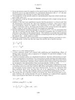
3. Aggregate demand and supply in r, Y Space
The relevant version of an aggregate demand and supply diagram in r, Y space is
illustrated in Fig. 15.1. In the figure, the C
d
(demand for commodities) or aggre-
gate demand schedule is negatively-sloped with respect to the real rate of inter-
est, and the supply curve, Y
s

, is positively-sloped. It should be stressed that this
formulation has little to do with Hicks’s (1937) IS/LM model, which deals only
with the demand side. There is an analogy between a standard IS curve and the
C
d
schedule. However, the C
d
,Y
s
construct omits any discussion of money, and
there is no analogue to the LM curve. The model exhibits a purely ‘real theory of
the real of interest’ as opposed to a ‘monetary theory of the real rate of interest’
(Burstein 1995). The upward slope of the aggregate supply function emerges as a
result of the new classical intertemporal substitution theory of labour supply,
whereby a higher interest rate supposedly stimulates more work effort.
In the present context, the most interesting feature of the re-labelling of the
axes, given that neither of the schedules has a vertical slope, is that (at least in
principle) there now appears to be some scope once again for effective demand
J. SMITHIN
152
Y
s
C
d
Y
0
r
*
r
Figure 15.1 An aggregate demand and supply diagram in r, Y space