Next generation wireless systems and networks phần 7 ppt

296 MULTIPLE ACCESS TECHNOLOGIES FOR B3G WIRELESS
As its name suggests, the system is based on OFDM, however, OFDMA is much more than just
a physical layer solution. It is a cross-layer-optimized technology that exploits the unique physical
properties of OFDM, enabling significant higher layer advantages that contribute to very efficient
packet data transmission in a cellular network.
Packet-switched air interface
The telephone network, designed basically for voice, is an example of circuit-switched systems.
Circuit-switched systems exist only at the physical layer that uses the channel resource to create an
end-to-end bit pipe. They are conceptually simple as the bit pipe is a dedicated resource, and the pipe
does not need to be controlled once it is created (some control may be required in setting up or tearing
down the pipe). Circuit-switched systems, however, are very inefficient for burst data traffic. Packet-
switched systems, on the other hand, are very efficient for data traffic but require that the upper layers
be controlled in addition to the physical layer that creates the bit pipe. The MAC layer is required for
the many data users to share the bit pipe. The data link layer is needed to take the error-prone pipe
and create a reliable link for the network layers to pass packet data flows over. The Internet is the best
example of a packet-switched network. Because all conventional cellular wireless systems, including
3G, were fundamentally designed for circuit-switched voice, they were designed and optimized pri-
marily at the physical layer. Some people suggested that the choice of CDMA as the physical layer
multiple access technology was also dictated by voice requirements. OFDMA, on the other hand, is a
packet-switched scheme designed for data and is optimized across the physical, MAC, data link, and
network layers. The choice of OFDM as the multiple access technology is based not only on physical
layer consideration, but also on the MAC layer, data link layer, and network layer requirements.
Physical layer advantages: OFDMA
As discussed earlier, most of the physical layer advantages of OFDM are well understood. Most
notably, OFDM creates a robust multiple access technology to deal with the impairments of the
wireless channel, such as multipath fading, delay spread, and Doppler shifts. Advanced OFDM-based
data systems typically divide the available spectrum into a number of equally spaced tones. For each
OFDM symbol duration, information carrying symbols (based on modulation such as QPSK, QAM,
etc.) are loaded on each tone.
The OFDMA can also use fast hopping across all tones in a predetermined pseudorandom pattern,
making it an SS technology. With fast hopping, a user that is assigned one tone does not transmit every

symbol on the same tone, but uses a hopping pattern to jump to a different tone for every symbol.
Different BSs use different hopping patterns, and each uses the entire available spectrum (thus to
realize frequency reuse of 1). In cellular deployment, this adds to the advantages of CDMA systems,
including frequency diversity and out of cell (intercell) interference averaging spectral efficiency
benefit that narrowband systems such as conventional TDMA do not have.
As discussed earlier, different users within the same cell use different resources (tones) and hence
do not interfere with each other. This is similar to TDMA, where different users in a cell transmit
at different time slots and do not interfere with one another. In contrast, CDMA users in a cell do
interfere with each other, increasing the total interference in the system. OFDMA therefore has the
physical layer benefits of both CDMA and TDMA and is at least three times (3times) more efficient
than CDMA. In other words, at the physical layer, OFDMA creates the biggest pipe of all cellular
technologies. Even though the 3times advantage at the physical layer is a huge advantage, the most
significant advantage of OFDMA for data is at the MAC and link layers.
MAC and link layer advantages
OFDMA exploits the granular nature of resources in OFDM to come up with extremely efficient
control layers. In OFDM, when designed appropriately, it is possible to send a very small amount
MULTIPLE ACCESS TECHNOLOGIES FOR B3G WIRELESS 297
(as little as one bit) of information from the transmitter to the receiver with virtually no overhead.
Therefore, a transmitter that is previously not transmitting can start transmitting as little as one bit of
information, and then stop, without causing any resource overhead. This is unlike CDMA or TDMA,
in which the granularity is much coarser, and merely initiating a transmission wastes a significant
resource. Hence, in TDMA, for example, there is a frame structure, and whenever a transmission
is initiated, a minimum of one frame (a few hundred bits) of information is transmitted. The frame
structure does not cause any significant inefficiency in user data transmission, as data traffic typically
consists of a large number of bits. However, for the transmission of control-layer information, the
frame structure is extremely inefficient, as the control information typically consists of one or two
bits but requires a whole frame. Not having a granular technology can therefore be very detrimental
from a MAC layer and link layer point of view.
OFDMA takes advantage of the granularity of OFDM in its control-layer design, enabling the
MAC layer to perform efficient packet switching over the air and at the same time provide all the

hooks to handle QoS. It also supports a data link layer that uses local (as opposed to end-to-end)
feedback to create a very reliable link from an unreliable wireless channel, with very low delays.
The network layer’s traffic therefore experiences small delays and no significant delay jitter. Hence,
interactive applications such as (packet) voice can be supported. Moreover, Internet protocols such
as TCP/IP run smoothly and efficiently over an OFDMA air link. As discussed in Chapter 3, TCP/IP
performance on 3G networks is very inefficient because the data link layer introduces significant delay
jitter so that channel errors are misinterpreted by TCP as network congestion and TCP responds by
backing off to the lowest rate.
Packet switching leads to efficient statistical multiplexing of data users and helps the wireless
operators to support a much greater number of users for a given user experience. This desirable feature
in OFDMA, together with QoS support and a three times bigger pipe, allows the operators to profitably
scale their wireless networks to meet the burgeoning data traffic demand in an all-you-can-eat pricing
environment.
7.6 Ultra-Wideband Technologies
As mentioned in Section 2.2.3, the UWB technology can be viewed as a derivative from the spreading
spectrum technology, in particular, the time hopping spread spectrum (THSS) technique, which is
also considered as a multiple access technology, being particularly suited for extreme narrow pulse
transmissions. Before discussing the technical details about the UWB technologies, we would like to
review briefly the history as well as the recent research activities carried out in this area.
Since the introduction of UWB technology to commercial applications in the early 1990s [674],
much of its initial research has been focused on the application of the THSS [675], where sev-
eral pulses in each symbol duration are sent with a particular time offset pattern determined by a
unique signature code for multiple access. The implementation of a THSS-UWB system requires a
precise network-wise synchronization clock. This inevitably increases overall hardware complexity
at a transceiver, which used to be a major concern in realizing a feasible UWB system at its early
stage. On the other hand, DS techniques can also work jointly with UWB systems to provide multiple
access among different users within the same wireless personal area network (WPAN). The operation
of a DS-UWB system does not need an accurate synchronization clock and the use of antipodal
pulses in DS modulation can boost up effective transmission power, which is very important to
improve the detection efficiency of a UWB receiver, due to the severe emission constraints imposed

on the power spectral mask specified in the FCC Part15.209, in which the maximal transmitting
power for a UWB transmitter should be lower than −41.3 dBm within the bandwidth from 3.1 to
10.6 GHz.
The UWB technologies have been standardized in IEEE 802.15.3a as a technology for WPANs.
Figure 7.18 shows all IEEE 802 standards, including those for WLANs as IEEE 802.11 standards,
298 MULTIPLE ACCESS TECHNOLOGIES FOR B3G WIRELESS
Figure 7.18 Various IEEE 802 standards, in which UWB technologies have been covered in IEEE
802.15.3a standard for WPAN applications.
wireless metropolitan area networks (WMANs) as IEEE 802.16 standards, WPANs as IEEE 802.15
standards, and so on. It is noted that IEEE 802.15.4.a is emerging as the standard for low-data-rate
transmission.
The FCC issued a notice of inquiry (NOI) in September 1998 and within a year the Time Domain
Corporation, US Radar, and Zircon Corporation had received waivers from the FCC to allow limited
deployment of a small number of UWB devices to support continued development of the technology,
and the University of Southern California (USC) UltRa Lab had an experimental licence to study
UWB radio transmissions. A notice of proposed rule making (NPRM) was issued in May 2000. In
April 2002, after extensive commentary from the industry, the FCC issued its first report and order
on UWB technology, thereby providing regulations to support deployment of UWB radio systems.
This FCC action was a major change in the approach to the regulation of RF emissions, allowing
a significant portion of the RF spectrum, originally allocated in many smaller bands exclusively for
specific uses, to be effectively shared with low-power UWB radios.
The FCC regulations classify UWB applications into several categories (see Table 7.5) with differ-
ent emission regulations in each case. Maximum emissions in the prescribed bands are at an effective
Table 7.5 The application categories specified by FCC UWB regulations
Application Frequency band for operation User limitations
at Part 1 limit
Communications and
measurement systems
3.1 to 10.6 GHz (different
out-of-band emission

limits for indoor and
outdoor devices)
No
Imaging: ground penetrating
radar, wall, medical
imaging
<960 MHz or 3.1 to
10.6 GHz
Yes
Imaging: through wall <960 MHz or 1.99 to
10.6 GHz
Yes
Imaging: surveillance 1.99 to 10.6 GHz Yes
Vehicular 24 to 29 GHz No
MULTIPLE ACCESS TECHNOLOGIES FOR B3G WIRELESS 299
−40
−45
−50
−55
−60
−65
−70
−75
0.96 1.61
1.99
3.1
10.6
GPS
10
0

10
1
Frequency in GHz
UMB EIRP Emission Level in dBm
−40
−45
−50
−55
−60
−65
−70
−75
0.96 1.61
1.99
3.1
10.6
GPS
10
0
10
1
Frequency in GHz
UMB EIRP Emission Level in dBm
Indoor Limit
Part 15 Limit
Outdoor Limit
Part 15 Limit
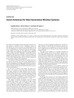
Figure 7.19 FCC regulated spectral masks regarding the indoor and outdoor UWB communications
applications.
Figure 7.20 Other communications applications in the vicinity of UWB operating bands.

isotropic radiated power (EIRP) of −41.3 dBm per MHz, and the −10 dB level of the emissions must
fall within the prescribed band, as shown in Figure 7.19, which should be compared with Figure 7.20
to know other communication applications in the vicinity of the UWB operating bands.
7.6.1 Major UWB Technologies
There are four major UWB technologies that have been proposed in the literature. The first type
is Time Hopped (TH) UWB or Time-modulated (TM) UWB,
1
which is a traditional UWB scheme
1
The traditional impulse radio technology can be called as either time hopped (TH) UWB or time modulated
(TM) UWB. It should be noted that both names are used very often.
300 MULTIPLE ACCESS TECHNOLOGIES FOR B3G WIRELESS
and is often called impulse radio (IR) UWB. The TH-UWB is by far the earliest version of UWB
technology and remains an important solution even today. The TH-UWB can be further divided into
two subcategories, that is, analog impulse radio multiple access (AIRMA) and digital impulse radio
multiple access (DIRMA), which were suggested and studied in [613, 624, 637]. The second UWB
technology is called direct-sequence CDMA-based UWB and can be implemented with a multi-carrier
CDMA architecture. The DS-CDMA UWB scheme will be discussed in detail in Subsections 7.6.1,
7.6.2, 7.6.3, 7.6.4, and 7.6.5. Another UWB scheme that has gained much popularity is based on
OFDM technology, namely, OFDM-UWB, which can be implemented on a multiband (MB) OFDM
scheme. The MB-OFDM UWB technology is particularly useful when cognitive radio technology is
used, as discussed in Chapter 9. In addition, some people also proposed frequency-modulation (FM)
based UWB systems, which can be implemented by swept frequency technology. Figure 7.21 shows
a family tree for all possible UWB technologies that have been proposed so far. Because of limited
space, we will only focus on the discussions on TH-UWB (or TM-UWB) and DS-CDMA UWB in
this subsection.
TH-UWB technology
The basic concept of a TH-UWB system is shown in Figure 7.22, where the system consists of
four major parts, namely, modulator
2

, delay unit, transmission time controller, and a pseudorandom
sequences generator. Obviously, in such a TH-UWB system, the data is sent in bursts and transmission
time is controlled by the pseudorandom sequences generator.
Understandably, the bandwidth of such a TM-UWB system is determined by the width and shape
of impulses, which usually takes some special waveforms, such as “monocycle.” The design of the
monocycles suitable for IR applications is a very interesting research topic in that the shape of the
monocycles should provide a very good time ACF for a better detection efficiency and fit FCC spectral
mask as illustrated in Figure 7.19. There are many pulse waveforms that have been proposed, such as
Gaussian pulse and its derivative functions, Hermite pulse and its modified versions, prolate spheroidal
waveforms, Laplacian monocycle, cubic monocycle, wavelets, and so on. For more information on
these popular impulses suitable for UWB applications, please refer to the large number of references
given at the end of this book [604–691].
Figure 7.21 Family tree for various UWB technologies proposed so far.
2
The most commonly used modulator scheme in an IR (or time hopping UWB) is pulse position modulation
(PPM), although many other modulation schemes can also be used, such as pulse amplitude modulation (PAM),
on-off-keying (OOK), pulse shape modulation (PSM), and so on.
MULTIPLE ACCESS TECHNOLOGIES FOR B3G WIRELESS 301
Figure 7.22 Block diagram for a TH-UWB IR transmitter.
The data signal should be sent out from an IR system, as shown in Figure 7.22, using carrier-
less transmission. The base band signal can be converted directly from the received signal and no
intermediate frequency unit is required, thus reducing the implementation complexity. The TM-UWB
scheme can provide a relatively large PG due to the fact that it has a very narrow impulse (whose
width is of the order of a nanosecond). This large PG also entails several other operational advantages,
which are explained as follows. First of all, it offers an excellent multipath immunity because of its
very high so time resolution that almost all multipath components can be separated and combined
coherently at a receiver. If the time between two pulses is longer than the channel delay spread,
there will be no ISI between two consecutive pulses, nor between two symbols.
3
Second, it gives a

good resistance to external interference based on the same reasons as any SS system. The big PG
also ensures a relatively low-power spectral density, which helps in not causing interference to other
existing wireless applications, as shown in Figure 7.20.
It is to be noted that the data-carrying modulation in an IR-UWB system is usually PPM, which
controls the appearance position of a pulse in a certain duration to represent different data-information.
On the other hand, the multiple access capability of an IR-UWB system is implemented through time
hopping schemes, as briefly discussed in Subsection 2.2.3. Different users in a pico-cell can be
assigned different PN sequences that control the timing of pulses, as shown in Figure 7.23, where
only three users are present for simplicity of illustration and 13 hopping slots are shown in one
symbol duration. In this case, there is no overlapping in the hopping slots among the three users,
implying that there will be no MAI.
A TH-UWB can offer a very good time diversity gain if multiple hopping patterns can be assigned
to a single user. Therefore, it is intuitively true that it can be made very robust against time-selective
fading, especially suitable for the applications where fast mobility is present.
4
DS-CDMA UWB technology
The direct-sequence CDMA UWB scheme is the focus of discussion in this subsection. The analysis
of a DS-CDMA UWB system is given in the following subsections. A DS-CDMA UWB scheme
works like a conventional DS-CDMA system. The pulse trains are used to perform DS modulation
to spread the signal. A PN code is assigned to a particular user and will be used to spread its data bit
into multiple chips. In the same way as in IR, various data modulation schemes, such as PAM, OOK,
PSM, and so on, can also be used in the DS-CDMA UWB system. Figure 7.24 shows an example
of the PAM-modulated DS-CDMA UWB scheme.
3
This is particularly true if a UWB system is operating in an indoor environment where the delay spread is
relatively small.
4
Because of the fact that most UWB systems are operated in an indoor environment, this advantage may not
be well exploited.
302 MULTIPLE ACCESS TECHNOLOGIES FOR B3G WIRELESS

U
U
U
Figure 7.23 Multiple access capability provided by a TH-UWB IR system.
Figure 7.24 Conceptual diagram of a DS-CDMA UWB system with PAM.
Many results have been reported on the performance of the DS-CDMA-based UWB systems, as
shown in [594–673]. Srinivasa [677] presents a comparison between a TH-PPM UWB and a TH
DS spreading with antipodal signaling (TH/DS-BPSK) in terms of their multiple access performance,
where the study was limited to an AWGN channel only. Foester [678] characterized the performance
of a direct sequence UWB system in the presence of multipath and narrowband interferences. It was
shown that the code design that tries to minimize sequence autocorrelation sidelobes as well as cross
correlation among spreading codes is critical for a good performance under multipath, multiuser, and
narrowband interferences at the same time.
A comprehensive review on almost all possible multiple access techniques suitable for UWB-
based WPANs or piconet was given in [679]. It was suggested that, among all multiple access schemes
(i.e. FDMA, TDMA, and CDMA), CDMA is the most suitable for UWB applications. The use of
CDMA allows multiple piconets to be relatively independent, and it is able to produce the highest
aggregate data rate. It was also pointed out that CDMA is completely compatible with high QoS,
MULTIPLE ACCESS TECHNOLOGIES FOR B3G WIRELESS 303
video streaming capable MAC layer protocols, such as the TDMA-based IEEE 802.15.3. On the
implementation side, to map to high-speed low-voltage low-power IC technologies, UWB systems
must use low peak-to-average pulse trains with a relatively high chip rate. These high chip rates are
perfectly suited for building UWB CDMA systems.
Qinghua Li and Rusch [680, 681] studied the effectiveness of an adaptive MMSE multiuser
detection for a DS-CDMA-based UWB system, particularly under the interference of an IEEE 802.11a
OFDM transmitter, as shown in Figure 7.20. Extensive simulations were performed using channel
sounding techniques in the 2- to 8-GHz band in a residential environment, which was characterized
by a high level of multipath fragmentation. It was demonstrated that the adaptive MMSE is able to
reject intersymbol and interchip interference for those channels much more effectively than by using
a RAKE receiver with four to eight fingers. It was also shown that the same receiver setting can

reject a narrowband interferer generated from an adjacent IEEE 802.11a transmitter. The majority of
the work was carried out on the basis of computer simulations.
Sadler and Swami [682] investigated a DS-UWB system with so-called episodic transmission,
that is, the system should send n pulses per information bit and allow for off time separation between
pulses. Several issues on the design of a DS-UWB system, such as PG, jamming margin, coding gain,
and multiple access interference, power control, and so on, were investigated. The BER performance
was studied using a Chernoff bound and considering a single-user matched-filter receiver in an AWGN
channel scenario.
The comparison between two UWB techniques for implementing multiple access communications,
specifically TH-PPM and DS-BPSK schemes, was made by Canadeo et al. [683]. They carried out a
spreading-code-dependent study on both UWB schemes. A generic channel model based on a very
simple delay tapped line was used. The coefficients in this multipath channel model were constants,
implying that no fading was considered.
Boudaker and Letaief [684] outlined the attractive features of DS-UWB multiple access systems
employing antipodal signaling and compared it with the TH scheme. An appropriate DS-UWB trans-
mitter and receiver were designed, and the system signal processing formulation was investigated.
The performance of such communication systems in an AWGN channel in terms of multiple access
capability, error rate performance, and achievable transmission rate were evaluated without MI. Only
a single matched-filter detector was considered.
An interesting method for implementing a DS-UWB system based on a new multi-carrier pulse
waveform was proposed in [685]. A unique frequency domain processing technique was used at the
receiver side to exploit diversity in the frequency domain and provide resistance against intersymbol
interference and multiple access interference. The performance of such a frequency domain processing
DS-UWB scheme was compared with a DS-UWB system using traditional time-domain processing
techniques.
An UWB system with PPM for data modulation and DS spreading for multiple access in an
indoor fading environment was considered in [686]. A RAKE receiver was used to combine a subset
of the resolvable multipath components using MRC technique. In the following subsections, we will
consider a multipath environment, modeled by a discrete-time linear filter with an impulse response
whose coefficients are lognormally distributed random variables.

Runkle et al. [688] compared a multi-carrier UWB with a DS-CDMA UWB. The results illustrated
that a significant advantage can be obtained if a UWB system is implemented by DS-CDMA tech-
niques. The multi-carrier UWB was implemented by a MB OFDM architecture. The authors explained
how the DS-CDMA UWB architecture could support robust and flexible multiuser capabilities, pro-
tect against in-band interference, and provide high resolution ranging capability for safety-of-life
applications.
A comparison of the average BER and outage probability performance of the three UWB multiple
access and modulation combinations for a single-user UWB radio was reported by [689]. The three
schemes are TH with bit flipping modulation, TH-PPM, and DS with bit flipping modulation. The
authors used the channel models recommended for use in the IEEE 802.15.3a evaluation. The results
304 MULTIPLE ACCESS TECHNOLOGIES FOR B3G WIRELESS
showed that direct sequence multiple access coding was more likely to achieve the lowest BER for
a fixed channel.
Unfortunately, most of the currently reported researches on UWB have separated the issues
on pulse waveform design from system-level performance, such as bit error probability, and so
on. In other words, the previous system-level analysis on BER performance seldom considered the
characteristic features of UWB pulses used in the system, as seen from all the papers referred in the
preceding text [675–689]. On the other hand, most of the current research on UWB pulse waveforms
was focused on the requirements concerning their spectral shapes and has little to do with the overall
system BER performance. In the following subsections, we demonstrate a BER performance analysis
that is associated with the characteristic feature of UWB pulse waveforms. We give a unified approach
to derive a closed form BER expression by taking into account major factors of a UWB system, such as
noninteger chip asynchronous transmission of the signals, multiple access interference, MI, and so on,
as well as their impact on the BER performance. In particular, we introduce a merit parameter, namely,
normalized mean squared autocorrelation function (NMSACF) of the pulse waveform denoted by
σ
2
mp
normal
. It will be used to characterize different UWB pulses in terms of their ACF. In fact,

σ
2
mp
normal
measures the average interchip interference level associated with the autocorrelation side
lobes of the pulse waveforms. We will illustrate from the analysis that σ
2
mp
normal
should be made as
small as possible to ensure a desirable BER performance.
7.6.2 DS-CDMA UWB System Model
Let us consider a DS-CDMA UWB radio system with K users. An ultranarrow pulse waveform g(t)
defined over
(
0,T
c
)
is used to directly modulate the binary data stream {b
(k)
j
}
k=1, ,K
j =−∞, ,∞
without
using a sinusoidal carrier. The k-th user is assigned a signature sequence {a
(k)
n
}
k=1, ,K

n=0, ,N−1
to modulate
antipodal pulses. Presumably, a pulse covers just a chip duration T
c
, and a signature code has N
chips such that T
b
= NT
c
,whereN is the PG.
The block diagram of this generic DS-CDMA UWB transceiver is shown in Figure 7.25, where
each transmitted signal will experience fading in the channel with its impulse response being h
k
(t) for
the k-th user. The receiver model is tuned to the first user’s transmitted signal with its signature code
being {a
(1)
n
}
N−1
n=0
. The received signal will be processed by signature code matched filtering as well
as pulse waveform–correlation before making a decision for the j-th bit, or at time t = (j + 1)T
b
.
The transmitted signal from the k-th user can be written as
s
k
(t) =
∞


j =−∞
N−1

n=0
b
(
k
)
j
a
(
k
)
n
g(t −jT
b
− nT
c
) (7.6)
where g(t) is defined as



g(t) = 0, 0 ≤ t ≤ T
c
g(t) = 0,t<0,t>T
c
max


g(t)

= 1, 0 ≤ t ≤ T
c
(7.7)
We are considering an asynchronous DS-CDMA UWB system and its pulse waveform–dependent
bit error performance analysis. The k-th user’s channel impulse response is h
k
(t) = αδ(t −τ
k
),where
α is a fading coefficient, which may obey any distribution dependent on a particular environment,
and δ(t −τ
k
) is an impulse function being unit at t = τ
k
and zero elsewhere. The received signal can
be expressed as
r(t) =
K

k=1
s
k
(t) ⊗ h
k
(t) + n(t) =
K

k=1

αs
k
(t −τ
k
) + n(t) (7.8)
where symbol ⊗ denotes the convolution operation, {τ
k
}
K
k=1
is the delay of the k-th user, n(t) obeys
Gaussian Distribution N(0,σ
2
n
) or can simply be denoted as n(t) ∼ N(0,σ
2
n
), which specifies a
MULTIPLE ACCESS TECHNOLOGIES FOR B3G WIRELESS 305
Figure 7.25 A block diagram of a DS-CDMA UWB transceiver. (a) Transmitter model; (b) Receiver
model, where the receiver is intended for user k and a flat fading channel is used.
relationship between n(t) and a Gaussian distribution with zero mean and variance σ
2
n
. Here, the
receiver intends to detect the first user’s transmission. Without loss of generality, let τ
1
= 0andτ
k
be the relative delay between the first and k-th users’ transmissions. Inserting s

k
(t) and h
k
(t) into
Equation (7.8), we obtain
r(t) =
∞

j =−∞
N−1

n=0
αb
(
1
)
j
a
(
1
)
n
g(t −jT
b
− nT
c
)
+
K


k=2
∞

j =−∞
N−1

n=0
αb
(
k
)
j
a
(
k
)
n
g(t −τ
k
− jT
b
− nT
c
) + n(t) (7.9)
The decision variable at the receiver can be written as
y

(
j + 1
)

T
b

=

(
j +1
)
T
b
jT
b
r(t)
N−1

n=0
a
(
1
)
n
g(t −jT
b
− nT
c
)dt = S +I +η (7.10)
306 MULTIPLE ACCESS TECHNOLOGIES FOR B3G WIRELESS
where decision variable y

(

j + 1
)
T
b

has been decomposed into three components, useful signal S,
multiple access interference I, and noise η. The useful signal component is written as
S =

(
j +1
)
T
b
jT
b
∞

j =−∞
N−1

n=0
αb
(
1
)
j
a
(
1

)
n
g(t −jT
b
− nT
c
)
N−1

n=0
a
(
1
)
n
g(t −jT
b
− nT
c
)dt
= αNb
(
1
)
j
E
mp
(7.11)
where E
mp

=

T
c
0
g
2
(
t
)
dt gives the energy of a single pulse. The MAI component can be expressed
by
I =
K

k=2
I
k
=
K

k=2

(
j +1
)
T
b
jT
b

∞

j =−∞
N−1

n=0
αb
(
k
)
j
a
(
k
)
n
g(t −τ
k
− jT
b
− nT
c
)
×
N−1

n=0
a
(
1

)
n
g(t −jT
b
− nT
c
)dt (7.12)
The noise term becomes
η =

(
j +1
)
T
b
jT
b
n(t)
N−1

n=0
a
(
1
)
n
g(t −jT
b
− nT
c

)dt (7.13)
As n(t) ∼ N

0,σ
2
n

,wehaveE
(
η
)
= 0 and the variance of η becomes
σ
2
η
= E

η
2

= E


(
j +1
)
T
b
jT
b

n(t)
N−1

n=0
a
(
1
)
n
g(t −jT
b
− nT
c
)dt

2
(7.14)
Letting q
(
t
)
=

N−1
n=0
a
(
1
)
n

g(t −jT
b
− nT
c
),weobtain
σ
2
η
= E

η
2

= E


(
j +1
)
T
b
jT
b
n(t)q
(
t
)
dt

2

=

(
j +1
)
T
b
jT
b

(
j +1
)
T
b
jT
b
E
[
n(t)n(ζ )
]
q
(
t
)
q
(
ζ
)
dt dζ

= σ
2
n

(
j +1
)
T
b
jT
b
N−1

n=0

a
(
1
)
n

2
g
2
1
(
t −jT
b
− nT
c

)
dt = σ
2
n
NE
mp
(7.15)
Therefore, we have η ∼ N

0,σ
2
n
NE
mp

.
7.6.3 Flat Fading Channel
In this subsection, we will proceed to determine the MAI term in a flat fading channel. In general,
the calculation of the variance of multiple access interference component I involves ACF of pulse
waveforms on a chip-by-chip basis, which is to be explained in the sequel.
MULTIPLE ACCESS TECHNOLOGIES FOR B3G WIRELESS 307
Chip-wise pulse autocorrelation function
Assume that the signal of interest is the first user’s transmission. Let us first consider the interference
component caused by the k-th transmission, which can be written as
I
k
=

(
j +1

)
T
b
jT
b
∞

j =−∞
N−1

n=0
αb
(
k
)
j
a
(
k
)
n
g(t −τ
k
− jT
b
− nT
c
)
N−1


n=0
a
(
1
)
n
g(t −jT
b
− nT
c
)dt (7.16)
The relative delay between the first and k-th users is τ
k
∈
(
0,T
b
)
, and two consecutive interfering
bits with respect to b
(1)
j
are b
(k)
j −1
and b
(k)
j
. We obtain
I

k
= α

(
j +1
)
T
b
jT
b


∞

j =−∞
N−1

n=0
b
(
k
)
j
a
(
k
)
n
g(t −τ
k

− jT
b
− nT
c
)


×
N−1

n=0
a
(1)
n
g(t −jT
b
− nT
c
)dt
= α

b
(
k
)
j −1

τ
k
0

N−1

n=0
a
(
k
)
n
g(t −τ
k
+ T
b
− nT
c
)
N−1

n=0
a
(
1
)
n
g(t −nT
c
)dt
+ b
(
k
)

j

T
b
τ
k
N−1

n=0
a
(
k
)
n
g(t −τ
k
− nT
c
)
N−1

n=0
a
(
1
)
n
g(t −nT
c
)dt


(7.17)
As shown in Appendix A, the k-th interfering component can be determined by
I
k
=

(
j +1
)
T
b
jT
b
∞

j =−∞
N−1

n=0
αb
(
k
)
j
a
(
k
)
n

g(t −τ
k
− jT
b
− nT
c
)
N−1

n=0
a
(
1
)
n
g(t −jT
b
− nT
c
)dt
= α

b
(
k
)
j −1

C
k,1

(
i
k
− N + 1
)

γ
k
T
c
0
g(t)g(t +
(
1 −γ
k
)
T
c
)dt
+ C
k,1
(
i
k
− N
)

T
c
γ

k
T
c
g(t)g(t −γ
k
T
c
)dt

+ b
(
k
)
j

C
k,1
(i
k
)

T
c
γ
k
T
c
g(t)g(t − γ
k
T

c
)dt
+ C
k,1
(i
k
+ 1)

γ
k
T
c
0
g(t)g(t +(1 −γ
k
)T
c
)dt

(7.18)
where γ
k
is the fractional-chip relative delay between the first and k-th users (as shown in Figure 7.26),
and C
k,1
(i) is the discrete aperiodic partial cross-correlation between signature codes of the first and
k-th users, which is defined as
C
k,1
(i) =


















N−1−i

j =0
a
(k)
j
a
(1)
j +i
, 0 ≤ i ≤ N − 1
N−1+i

j =0

a
(k)
j −i
a
(1)
j
, −(N −1) ≤ i ≤ 0
0, otherwise
(7.19)
Let us define chip-wise pulse waveform autocorrelation function as
R
p
(
τ
)
=

T
c
−T
c
g(t)g(t −τ)dt (7.20)
308 MULTIPLE ACCESS TECHNOLOGIES FOR B3G WIRELESS
Figure 7.26 Calculation of asynchronous cross-correlation function with fractional-chip delay, that
is, τ
k
= (j + γ
k
)T
c

, between transmitting signals from the first and k-th users, where γ
k
takes a real
value such that 0 ≤ γ
k
≤ 1.
Thus,wehave
R
p
(
γ
k
T
c
)
=

T
c
γ
k
T
c
g(t)g(t − γ
k
T
c
)dt (7.21)
R
p

(
−
(
1 −γ
k
)
T
c
)
=

γ
k
T
c
0
g(t)g(t +T
c
− γ
k
T
c
)dt (7.22)
The illustrations of R
p
(
γ
k
T
c

)
and R
p
(
−
(
1 −γ
k
)
T
c
)
have been given in Figure 7.27. Therefore, the
k-th interfering component can be written as
I
k
= α

b
(
k
)
j −1

C
k,1
(
i
k
− N + 1

)
R
p
(
−
(
1 −γ
k
)
T
c
)
+ C
k,1
(
i
k
− N
)
R
p
(
γ
k
T
c
)

+ b
(

k
)
j

C
k,1
(
i
k
)
R
p
(
γ
k
T
c
)
+ C
k,1
(
i
k
+ 1
)
R
p
(
−
(

1 −γ
k
)
T
c
)


(7.23)
which contains four random variables. b
(k)
j −1
and b
(k)
j
are two consecutive bits of the k-th user, γ
k
is
the fractional-chip relative delay between the first and k-th users, and α is the flat fading coefficient
of the channel. Theoretically speaking, if we know the distributions of all four random variables, it is
possible to obtain the distribution of I
k
from Equation (7.23), and thus the distribution of I =

K
k=2
I
k
by convolution of f
I

(x) = f
I
2
⊗ f
I
3
⊗ ⊗ f
I
K
. Unfortunately, the intricate relationship between
the four random variables in Equation (7.23) makes it almost impossible to calculate explicitly the
distribution of I
k
. Therefore, we will use the Gaussian approximation to obtain the close form of
BER.
MULTIPLE ACCESS TECHNOLOGIES FOR B3G WIRELESS 309
Figure 7.27 This figure illustrates how to calculate chip-wise pulse autocorrelation functions R
p
(γ
k
T
c
)
and R
p
(−(1 −γ
k
)T
c
).

MAI statistics in a flat fading channel
If K is sufficiently large, we can approximate the multiple access interference term, that is, I ,asa
Gaussian random variable. Therefore, the decision variable y

(j + 1)T
b

defined in Equation (7.10)
will also be Gaussian. It is assumed that the appearance frequency of two consecutive bits for the
k-th user is independently equiprobable; that is, P(b
(k)
j
= 1) = P(b
(k)
j
=−1) =
1
2
. Besides, we also
have
E

(b
(k)
j −1
)
2

= E


(b
(k)
j
)
2

= 1; E

b
(k)
j −1
b
(k)
j

= E

b
(k)
j −1
)E(b
(k)
j

= 0 · 0 = 0 (7.24)
Therefore, the conditional mean of I
k
can be calculated as
E
(

I
k
|i
k
,γ
k
)
=
1
2
α

C
k,1
(
i
k
− N + 1
)
R
p

−
(
1 −γ
k
)
T
c


+ C
k,1
(
i
k
− N
)
R
p
(
γ
k
T
c
)
+ C
k,1
(
i
k
)
R
p
(
γ
k
T
c
)
+ C

k,1
(
i
k
+ 1
)
R
p

−
(
1 −γ
k
)
T
c

+
1
2
α
c

C
k,1
(
i
k
− N + 1
)

R
p

−
(
1 −γ
k
)
T
c

+ C
k,1
(
i
k
− N
)
R
p
(
γ
k
T
c
)
− C
k,1
(
i

k
)
R
p
(
γ
k
T
c
)
− C
k,1
(
i
k
+ 1
)
R
p

−
(
1 −γ
k
)
T
c

= α


C
k,1
(
i
k
− N + 1
)
R
p

−
(
1 −γ
k
)
T
c

+ C
k,1
(
i
k
− N
)
R
p
(
γ
k

T
c
)

(7.25)
Using the results given in Equation (7.24), we obtain the conditional second order moment of I
k
as
E

I
2
k
|i
k
,γ
k

= α
2


C
k,1
(
i
k
− N +1
)
R

p
(
−
(
1 −γ
k
)
T
c
)
+ C
k,1
(
i
k
− N
)
R
p
(
γ
k
T
c
)

2
+

C

k,1
(
i
k
)
R
p
(
γ
k
T
c
)
+ C
k,1
(
i
k
+ 1
)
R
p
(
−
(
1 −γ
k
)
T
c

)

2

(7.26)
310 MULTIPLE ACCESS TECHNOLOGIES FOR B3G WIRELESS
Therefore, the conditional variance of I
k
becomes
Var
(
I
k
|i
k
,γ
k
)
= E

I
2
k
|i
k
,γ
k

−


E
(
I
k
|i
k
,γ
k
)

2
= α
2

C
k,1
(
i
k
)
R
p
(
γ
k
T
c
)
+ C
k,1

(
i
k
+ 1
)
R
p

−
(
1 −γ
k
)
T
c

2
(7.27)
Because of I =

K
k=2
I
k
, we have the conditional mean of I as
E
(
I |i, γ
)
=

K

k=2
E
(
I
k
|i
k
,γ
k
)
=
K

k=2
α

C
k,1
(
i
k
− N + 1
)
R
p

−
(

1 −γ
k
)
T
c

+ C
k,1
(
i
k
− N
)
R
p
(
γ
k
T
c
)

(7.28)
We also have
I
2
=
K

k=2

I
2
k
+
K

x=2
K

x=y,y=2
I
x
I
y
(7.29)
If all interference components, that is, I
2
, ,I
K
, are mutually independent, the conditional variance
can be written as
Var
(
I |i, γ
)
= E

I
2
|i

k
,γ
k

−

E
(
I |i
k
,γ
k
)

2
=
K

k=2
E

I
2
k
|i
k
,γ
k

+

K

x=2
K

x=y,y=2
E
(
I
x
|i
x
,γ
x
)
E

I
y
|i
y
,γ
y

−
K

k=2
E
2

(
I
k
|i
k
,γ
k
)
−
K

x=2
K

x=y,y=2
E
(
I
x
|i
x
,γ
x
)
E

I
y
|i
y

,γ
y

=
K

k=2
E

I
2
k
|i
k
,γ
k

−
K

k=2
E
2
(
I
k
|i
k
,γ
k

)
(7.30)
Therefore we obtain
Var
(
I |i, γ
)
=
K

k=2
E

I
2
k
|i
k
,γ
k

−
K

k=2
E
2
(
I
k

|i
k
,γ
k
)
=
K

k=2
α
2

C
k,1
(
i
k
− N + 1
)
R
p

−
(
1 −γ
k
)
T
c


+ C
k,1
(
i
k
− N
)
R
p
(
γ
k
T
c
)

2
+

C
k,1
(
i
k
)
R
p
(
γ
k

T
c
)
+ C
k,1
(
i
k
+ 1
)
R
p

−
(
1 −γ
k
)
T
c

2

−
K

k=2
α
2


C
k,1
(
i
k
− N + 1
)
R
p

−
(
1 −γ
k
)
T
c

+ C
k,1
(
i
k
− N
)
R
p
(
γ
k

T
c
)

2
=
K

k=2
α
2

C
k,1
(
i
k
)
R
p
(
γ
k
T
c
)
+ C
k,1
(
i

k
+ 1
)
R
p

−
(
1 −γ
k
)
T
c

2
(7.31)
MULTIPLE ACCESS TECHNOLOGIES FOR B3G WIRELESS 311
from which we observe that the variance of the combined interference component is closely related
to three parameters; one being the square of the fading coefficient α, the other being the partial CCF
of the signature codes of the first and k-th users, and the last being the ACF of UWB pulse waveform
R
p
(γ
k
T
c
) and R
p

−

(
1 −γ
k
)
T
c

. In fact, both partial cross-correlation function of the signature
codes and ACF of the pulse waveform can be calculated explicitly if we have the knowledge of user
signature codes and pulse waveforms, and thus the variance of MAI can also be determined.
Random sequences
In this subsection, purely random sequences will be used as spreading sequences, whose chips
{a
(k)
n
}
k=1, ,K
n=0, ,N−1
will take “−1” and “+1” equally likely. In addition, a
(k)
i
and a
(k)
j
should be indepen-
dent if i = j . The integer-chip relative delay between the first and k-th users’ transmissions, {i
k
}
K
k=1

,
is uniformly distributed over (0,N − 1); and the fractional-chip relative delay between the first and
k-th users’ transmissions, {γ
k
}
K
k=1
, is uniformly distributed over (0, 1). On the basis of these assump-
tions, we can calculate the unconditional expectation of discrete partial cross-correlation functions of
the first and k-th spreading sequences as follows:















E

C
k,1
(

i
)
|i

= E


N−1−i

j =0
a
(k)
j
a
(1)
j +i


= 0, 0 ≤ i ≤ N − 1
E

C
k,1
(
i
)
|i

= E



N−1+i

j =0
a
(k)
j −i
a
(1)
j


= 0, −(N −1) ≤ i ≤ 0
(7.32)
The unconditional second order moment of discrete partial CCFs can be calculated section by
section as
E


C
k,1
(
i
)

2
|i

= E



N−1−i

l=0
N−1−i

j =0
a
(k)
j
a
(1)
j +i
a
(k)
l
a
(1)
l+i


=
N−1−i

l=0
N−1−i

j =0
E


a
(k)
j
a
(1)
j +i
a
(k)
l
a
(1)
l+i

=
N−1−i

l=0
N−1−i

j =0
E

a
(1)
j +i
a
(1)
l+i

E


a
(k)
j
a
(k)
l

=
N−1−i

j =0
E


a
(1)
j +i

2

E


a
(k)
j

2


= N −i,
(
0 ≤ i ≤ N − 1
)
(7.33)
and
E


C
k,1
(
i
)

2
|i

= E


N−1+i

l=0
N−1+i

j =0
a
(k)
j −i

a
(1)
j
a
(k)
l−i
a
(1)
l


=
N−1+i

l=0
N−1+i

j =0
E

a
(k)
j −i
a
(1)
j
a
(k)
l−i
a

(1)
l

312 MULTIPLE ACCESS TECHNOLOGIES FOR B3G WIRELESS
=
N−1+i

l=0
N−1+i

j =0
E

a
(k)
j −i
a
(k)
l−i

E

a
(1)
j
a
(1)
l

=

N−1+i

j =0
E


a
(k)
j −i

2

E


a
(1)
j

2

= N +i,
[
−(N −1) ≤ i ≤ 0
]
(7.34)
Inserting the above results into Equation (7.28), we obtain
E
(
I |γ

)
= E

E
(
I |i, γ
)

=
K

k=2
N−1

i
k
=0
α
N

E

C
k,1
(
i
k
− N + 1
)


R
p
(
−
(
1 −γ
k
)
T
c
)
+ E

C
k,1
(
i
k
− N
)

R
p
(
γ
k
T
c
)


= 0 (7.35)
Applying Equations (7.33) and (7.34) to Equation (7.31), we have
Var
(
I |γ
)
= E

Var
(
I |i, γ
)

=
K

k=2
N−1

i
k
=0
1
N
α
2
E


C

k,1
(
i
k
)
R
p
(
γ
k
T
c
)
+ C
k,1
(
i
k
+ 1
)
R
p
(
−
(
1 − γ
k
)
T
c

)

2

=
K

k=2
N−1

i
k
=0
1
N
α
2

(
N −i
k
)

R
p
(
γ
k
T
c

)

2
+
(
N −i
k
− 1
)

R
p
(
−
(
1 −γ
k
)
T
c
)

2

=
K

k=2
α
2


(
N +1
)
2

R
p
(
γ
k
T
c
)

2
+
(
N −1
)
2

R
p
(
−
(
1 −γ
k
)

T
c
)

2

(7.36)
Let us define parameter σ
2
mp
as
σ
2
mp
= E

R
2
p
(
τ
)

=
1
2T
c

T
c

−T
c


T
c
−T
c
g(t −τ)g(t)dt

2
dτ, (7.37)
then we have
Var
(
I
)
= E

Var
(
I |γ
)

=
K

k=2
α
2


(
N +1
)
2
E


R
p
(
γ
k
T
c
)

2

+
(
N −1
)
2
E


R
p
(

−
(
1 −γ
k
)
T
c
)

2


=
(
K −1
)
α
2
Nσ
2
mp
(7.38)
Now that we have identified all deterministic and random components in the decision variable as





S = αNb
(

1
)
j
E
mp
η ∼ N

0,σ
2
n
NE
mp

I ∼ N

0,
(
K −1
)
α
2
Nσ
2
mp

,
(7.39)
together with the decision rule of
z
(

j
)
=

+1,y
((
j + 1
)
T
b
)
> 0
−1,y
((
j + 1
)
T
b
)
≤ 0,
(7.40)
MULTIPLE ACCESS TECHNOLOGIES FOR B3G WIRELESS 313
we can proceed to derive the BER expression as
P
e
=

∞
−∞
Q






αNE
mp

σ
2
n
NE
mp
+
(
K −1
)
α
2
Nσ
2
mp





f
α
(α) dα

=

∞
−∞
Q







1

1
α
2
σ
2
n
NE
mp
+
(
K −1
)
σ
2
mp
NE

2
mp







f
α
(α) dα
=

∞
−∞
Q







1

1
α
2
1

SNR
+
(
K −1
)
σ
2
mp
normal
NE
mp







f
α
(α) dα (7.41)
where σ
2
mp
normal
has been defined as
σ
2
mp
normal

=
σ
2
mp
E
mp
(7.42)
and f
α
(α) is the probability density function of fading coefficient α.
7.6.4 Frequency-Selective Fading Channels
In this subsection, we analyze pulse waveform–dependent BER performance of a DS-CDMA UWB
radio under a frequency-selective fading environment. The multipath fading channel is modeled by a
modified Saleh–Valenzuela (S–V) indoor channel model, which was initially proposed by A. Saleh
and R. Valenzuela [690] and was modified by J. Foerster and Q. Li [691].
Modified S–V channel model
The basic idea of the modified S–V channel model can be summarized as follows [691].
• The signal arrivals from an indoor channel can be decomposed into several clusters, each of
which consists of several multipath rays. Different clusters are formed because of the building’s
structure, such as different storeys; while different rays in the same cluster are formed owing
to different reflecting objects in the propagation path of the cluster.
• The amplitude of the rays attenuates according to a Lognormal distribution (instead of a
Rayleigh Distribution as suggested in the original S–V model [690]). In addition, the vari-
ance of amplitude attenuation decays exponentially with the delays of different clusters as well
as different rays in the same cluster.
• The arrival processes of both clusters and rays obey Poisson distributions and thus their interar-
rival times are exponentially (instead of uniform, as specified in the original S–V model [690])
distributed.
The modified S–V channel model can be expressed mathematically by
h

(
t
)
=
Q

q=1
L

l=1
w
q,l
α
q,l
δ

t −T
q
− τ
q,l

(7.43)
314 MULTIPLE ACCESS TECHNOLOGIES FOR B3G WIRELESS
where q ∈ (1,Q) and l ∈ (1,L) stand for cluster and ray indices, respectively; {w
q,l
}
q=1, ,Q
l=1, ,L
takes
either +1or−1 to denote either positive or negative path return; {T

q
}
Q
q=1
is the delay of the first ray
in the q-th cluster; {τ
q,l
}
q=1, ,Q
l=1, ,L
is the relative delay between the first and l-th rays in the q-th cluster
with T
1
= 0and{τ
q,1
}
Q
q=1
= 0, without losing generality. To model the exponential distributions of
interarrival times for both clusters and rays, we need to define two parameters,  and λ,which
represent cluster arrival rate and ray arrival rate, respectively, with their distributions being

p

T
q
|T
q−1

=  exp


−

T
q
− T
q−1

,q>0
p

τ
q,l
|τ
q,l−1

= λ exp

−λ

τ
q,l
− τ
q,l−1

,l>0
(7.44)
Because of the properties of exponentially distributed interarrival times for both clusters and rays,
we have


T
q
− T
1
=

T
q
− T
q−1

+

T
q−1
− T
q−2

+···+
(
T
2
− T
1
)
τ
q,l
− τ
q,1
=


τ
q,l
− τ
q,l−1

+

τ
q,l−1
− τ
q,l−2

+···+

τ
q,2
− τ
q,1

(7.45)
and thus the mean interarrival times for both clusters and rays can be expressed by

E

T
q

=
(

q − 1
)
1

E

τ
q,l

=
(
l − 1
)
1
λ
(7.46)
The mean relative delay between the l-th ray in the q-th cluster and the first ray in the first cluster
is
E

T
q
+ τ
q,l

=
(
q − 1
)
1


+
(
l − 1
)
1
λ
(7.47)
The channel gain α
q,l
is a Lognormal random variable, whose relation can be written as
20 log
10

α
q,l

∼ N

µ
q
,σ
2

(7.48)
Also, α
q,l
in Equation (7.43) is always positive and its second order moment obeys a dual-
exponential distribution as
E


α
2
q,l

= 
1
e
−T
q
/
e
−τ
q,l
/γ
(7.49)
where  and γ are the attenuation coefficients for the clusters and rays, respectively; 
1
is the mean
power of the first ray in the first cluster. Therefore, the mean of α
q,l
in Equation (7.48) can be written
as
µ
q
=
10 ln
(

1

)
− 10T
q
/ −10τ
q.l
/γ
ln
(
10
)
−
σ
2
ln
(
10
)
20
(7.50)
Received signal in modified S– V channel
The transmitter block diagram for a DS-CDMA UWB radio under frequency-selective fading chan-
nels is almost exactly the same as Figure 7.25(a). The only difference is that the channel impulse
responses {h
k
(t)}
K
k=1
in Figure 7.25(a) should be replaced by the modified S–V model defined in
Equation (7.43), or
h

k
(
t
)
=
Q
k

q=1
L
k

l=1
w
k,q,l
α
k,q.l
δ

t −T
k,q
− τ
k,q,l
− τ
k

; (7.51)
where {τ
k
}

K
k=1
is the relative delay between the first and k-th users’ transmissions and τ
1
= 0. The
receiver model is shown in Figure 7.28, where a RAKE receiver is used for the reception of the
signal from user 1. The transmitted signal from the k-th user can be written as
s
k
(
t
)
=
∞

j =−∞
N−1

n=0
b
(
k
)
j
a
(
k
)
n
g(t −jT

b
− nT
c
) (7.52)
MULTIPLE ACCESS TECHNOLOGIES FOR B3G WIRELESS 315
Figure 7.28 The RAKE receiver for reception of the signal from the first user using the modified
S–V channel model, where there are totally L
1
fingers, the combining coefficients are {β
p
}
L
1
p=1
,and
τ
1,1
= 0 without losing generality.
where {b
(k)
j
}
K
k=1
is the input binary information from the k-th user, T
b
is the bit duration, {a
(k)
n
}

N−1
n=0
is the spreading sequence for the k-th user with its length being N, T
c
is the chip duration with
T
b
= NT
c
,andg(t) denotes the pulse waveform, which was defined in Equation (7.7).
The received signal can be written as
r(t) =
K

k=1
s
k
(t) ⊗ h
k
(
t
)
+ n(t)
=
K

k=1
Q
k


q=1
L
k

l=1
w
k,q,l
α
k,q,l
s
k

t −T
k,q
− τ
k,q,l
− τ
k

+ n(t) (7.53)
where ⊗ denotes convolution operation; n(t) is the AWGN component added in the channel with its
mean and variance being zero and σ
2
n
, respectively, or simply represented by n(t) ∼ N(0,σ
2
n
).After
the convolution, the received signal can be rewritten as
r(t) =

Q
1

q=1
L
1

l=1
∞

j =−∞
N−1

n=0
w
q,l
α
q,l
b
(
1
)
j
a
(
1
)
n
g(t −T
q

− τ
q,l
− jT
b
− nT
c
)
+
K

k=2
Q
k

q=1
L
k

l=1
∞

j =−∞
N−1

n=0
w
k,q,l
α
k,q,l
b

(
k
)
j
a
(
k
)
n
g(t −T
k,q
− τ
k,q,l
− τ
k
− jT
b
− nT
c
)
+ n(t) (7.54)
316 MULTIPLE ACCESS TECHNOLOGIES FOR B3G WIRELESS
It is assumed that an L
1
-finger RAKE receiver will capture the L
1
rays in the first cluster multipath
returns. The output from the p-th finger is
y
p


τ
1,p
+
(
j + 1
)
T
b

=

τ
1,p
+
(
j +1
)
T
b
τ
1,p
+jT
b
r(t)β
p
N−1

n=0
a

(
1
)
n
g(t −τ
1,p
− jT
b
− nT
c
)dt (7.55)
Then, the decision variable for the j-th bit, v(j), becomes
v(j) =
L
1

p=1
y
l

τ
1,p
+
(
j + 1
)
T
b

=

L
1

p=1

τ
1,p
+
(
j +1
)
T
b
τ
1,p
+jT
b
r(t)β
p
N−1

n=0
a
(
1
)
n
g(t −τ
1,p
− jT

b
− nT
c
)dt (7.56)
which can be decomposed into four terms, that is, useful signal, MI, MAI, and noise, as
v(j) = S +I
L
+ I
K
+ η =
L
1

p=1

S
p
+ I
L,p
+ I
K,p
+ η
p

(7.57)
where S
p
, I
L,p
, I

K,p
,andη
p
are the useful signal, MI, MAI, and noise terms generated from the
p-th finger, respectively. The useful signal component can be written as
S
p
=

τ
1,p
+
(
j +1
)
T
b
τ
1,p
+jT
b
β
p
∞

j =−∞
N−1

n=0
w

1,p
α
1,p
b
(
1
)
j
a
(
1
)
n
g(t −τ
1,p
− jT
b
− nT
c
)
×
N−1

n=0
a
(
1
)
n
g(t −τ

1,p
− jT
b
− nT
c
)dt
= β
p
w
1,p
α
1,p
Nb
(
1
)
j
E
mp
(7.58)
where E
mp
=

T
c
0
g
2
(

t
)
dt denotes the energy of a single pulse. The weighted sum of the useful
signal component yields
S =
L
1

p=1
S
p
= Nb
(
1
)
j
E
mp
L
1

p=1
β
p
w
1,p
α
1,p
(7.59)
AW GN s ta tis ti c s

The noise component from the first finger can be written as
η
1
=

(
j +1
)
T
b
jT
b
β
1
n(t)
N−1

n=0
a
(
1
)
n
g(t −jT
b
− nT
c
)dt (7.60)
Obviously, since n(t) ∼ N


0,σ
2
n

we readily get E
(
η
1
)
= 0 from Equation (7.60). The variance of
the noise component from the first finger can be calculated as
σ
2
η
1
= E

η
2
1

= E


(
j +1
)
T
b
jT

b
β
1
n(t)
N−1

n=0
a
(
1
)
n
g(t −jT
b
− nT
c
)dt

2
(7.61)
MULTIPLE ACCESS TECHNOLOGIES FOR B3G WIRELESS 317
Let q
(
t
)
= β
1

N−1
n=0

a
(
1
)
n
g(t −jT
b
− nT
c
). Equation (7.61) can be written as
σ
2
η
1
= E

η
2
1

= E


(
j +1
)
T
b
jT
b

n(t)q
(
t
)
dt

2
=

(
j +1
)
T
b
jT
b

(
j +1
)
T
b
jT
b
E
[
n(t)n(ζ )
]
q
(

t
)
q
(
ζ
)
dt dζ
= σ
2
n

(
j +1
)
T
b
jT
b
q
2
(
t
)
dt = σ
2
n

(
j +1
)

T
b
jT
b
β
2
1
N−1

n=0

a
(
1
)
n

2
g
2
1
(
t −jT
b
− nT
c
)
dt
= σ
2

n
β
2
1
NE
mp
(7.62)
Therefore, the noise term in the output from the first finger is still Gaussian as η
1
∼ N

0,σ
2
n
β
2
1
NE
mp

.
The weighted sum of all noise terms in the output of the RAKE receiver will be Gaussian too, or
η ∼ N


0,σ
2
n
NE
mp

L
1

p=1
β
2
p


(7.63)
MI statistics in modified S–V channel
From Equation (7.57) we have the MI component in the decision variable v(j) as I
L
=

L
1
p=1
I
L,p
.
It is known from Equations (7.54) and (7.56) that the MI term obtained from the output of the first
finger is
I
L,1
=
L
1

l=2

I
1,l,1
+
Q
1

q=2
L
1

l=1
I
q,l,1
=
L
1

l=2

(
j +1
)
T
b
jT
b
β
1
w
1,l

α
1,l
∞

j =−∞
N−1

n=0
b
(
1
)
j
a
(
1
)
n
g(t −τ
1,l
− jT
b
− nT
c
)
×
N−1

n=0
a

(1)
n
g(t −jT
b
− nT
c
)dt
+
Q
1

q=2
L
1

l=1

(
j +1
)
T
b
jT
b
β
1
w
q,l
α
q,l

∞

j =−∞
N−1

n=0
b
(
1
)
j
a
(
1
)
n
g(t −T
q
− τ
q,l
− jT
b
− nT
c
)
×
N−1

n=0
a

(1)
n
g(t −jT
b
− nT
c
)dt (7.64)
Using the approach as shown in Appendix B, we can obtain
I
L,1
=
L
1

l=2
I
1,l,1
+
Q
1

q=2
L
1

l=1
I
q,l,1
=
L

1

l=2
β
1
w
1,l
α
1,l

b
(
1
)
j −1

C
1

i
1,l
− N +1

R
p

−

1 −γ
1,l


T
c

+ C
1

i
1,l
− N

R
p

γ
1,l
T
c

318 MULTIPLE ACCESS TECHNOLOGIES FOR B3G WIRELESS
+ b
(
1
)
j

C
1

i

1,l

R
p

γ
1,l
T
c

+ C
1

i
1,l
+ 1

R
p

−

1 −γ
1,l

T
c


+

Q
1

q=2
L
1

l=1
β
1
w
q,l
α
q,l

b
(
1
)
j −1

C
1

i
q,l
− N + 1

R
p


−

1 −γ
q,l

T
c

+ C
1

i
q,l
− N

R
p

γ
q,l
T
c

+ b
(
1
)
j


C
1

i
q,l

R
p

γ
q,l
T
c

+ C
1

i
q,l
+ 1

R
p

−

1 −γ
q,l

T

c


(7.65)
Similarly, we can also have
I
L,p
=
L
1

l=1,l=p
I
1,l,p
+
Q
1

q=2
L
1

l=1
I
q,l,p
=
L
1

l=1,l=p

β
p
w
1,l
α
1,l

b
(
1
)
j −1

C
1

i
1,l,p
− N + 1

R
p

−

1 −γ
1,l,p

T
c


+ C
1
(i
1,l,p
− N)R
p
(γ
1,l,p
T
c
)

+ b
(
1
)
j

C
1

i
1,l,p

R
p

γ
1,l,p

T
c

+ C
1

i
1,l,p
+ 1

R
p

−

1 −γ
1,l,p

T
c


+
Q
1

q=2
L
1


l=1
β
p
w
q,l
α
q,l

b
(
1
)
j −1

C
1

i
q,l,p
− N +1

R
p

−

1 −γ
q,l,p

T

c

+ C
1
(i
q,l,p
− N)R
p
(γ
q,l,p
T
c
)

+ b
(
1
)
j

C
1

i
q,l,p

R
p

γ

q,l,p
T
c

+ C
1

i
q,l,p
+ 1

R
p

−

1 −γ
q,l,p

T
c


(7.66)
Assume that the first user sends its binary bit stream with “+1” and “−1” appearing equal
likely or P(b
(
1
)
j

= 1) = P(b
(
1
)
j
=−1) =
1
2
, and thus E{[b
(1)
j −1
]
2
}=E{[b
(1)
j
]
2
}=1andE[b
(1)
j −1
b
(1)
j
] =
E[b
(1)
j −1
]E[b
(1)

j
] = 0 ·0 = 0. From Equation (7.66) we can proceed to derive the conditional mean and
variance of I
1,l,1
, which corresponds to the signal captured from the l-th ray in the first cluster of the
first user, as
E

I
1,l,1
|i
1,l,1
,γ
1,l,1
,w
1,l
,α
1,l
,β
1

= β
1
w
1,l
α
1,l

C
1


i
1,l,1
− N + 1

R
p

−

1 −γ
1,l,1

T
c

+ C
1

i
1,l,1
− N

R
p

γ
1,l,1
T
c


Var

I
1,l,1
|i
1,l,1
,γ
1,l,1
,w
1,l
,α
1,l
,β
1

= β
2
1
w
2
1,l
α
2
1,l

C
1

i

1,l,1

R
p

γ
1,l,1
T
c

+ C
1

i
1,l,1
+ 1

R
p

−

1 −γ
1,l,1

T
c

2
Similarly, we can derive the conditional mean and variance for the signal captured from the l-th

rayintheq-th cluster of the first user as
E

I
q,l,1
|i
q,l,1
,γ
q,l,1
,w
q,l
,α
q,l
,β
1

= β
1
w
q,l
α
q,l

C
1

i
q,l,1
− N + 1


R
p

−

1 −γ
q,l,1

T
c

+ C
1

i
q,l,1
− N

R
p

γ
q,l,1
T
c

Var

I
q,l,1

|i
q,l,1
,γ
q,l,1
,w
q,l
,α
q,l
,β
1

= β
2
1
w
2
q,l
α
2
q,l

C
1

i
q,l,1

R
p


γ
q,l,1
T
c

+ C
1

i
q,l,1
+ 1

R
p

−

1 −γ
q,l,1

T
c

2
MULTIPLE ACCESS TECHNOLOGIES FOR B3G WIRELESS 319
Therefore, the conditional mean and variance of the MI term from the first finger become
E

I
L,1

|i
q,l,1
,γ
q,l,1
,w
q,l
,α
q,l
,β
1

=
L
1

l=2
E

I
1,l,1
|i
1,l,1
,γ
1,l,1
,w
1,l
,α
1,l
,β
1


+
Q
1

q=2
L
1

l=1
E

I
q,l,1
|i
q,l,1
,γ
q,l,1
,w
q,l
,α
q,l
,β
1

=
L
1

l=2

β
1
w
1,l
α
1,l

C
1

i
1,l,1
− N + 1

R
p

−

1 −γ
1,l,1

T
c

+ C
1

i
1,l,1

− N

R
p

γ
1,l,1
T
c

+
Q
1

q=2
L
1

l=1
β
1
w
q,l
α
q,l

C
1

i

q,l,1
− N + 1

R
p

−

1 −γ
q,l,1

T
c

+ C
1

i
q,l,1
− N

R
p

γ
q,l,1
T
c

(7.67)

Var

I
L,1
|i
q,l,1
,γ
q,l,1
,w
q,l
,α
q,l
,β
1

=
L
1

l=2
Var

I
1,l,1
|i
1,l,1
,γ
1,l,1
,w
1,l

,α
1,l
,β
1

+
Q
1

q=2
L
1

l=1
Var

I
q,l,1
|i
q,l,1
,γ
q,l,1
,w
q,l
,α
q,l
,β
1

=

L
1

l=2
β
2
1
w
2
1,l
α
2
1,l

C
1

i
1,l,1

R
p

γ
1,l,1
T
c

+ C
1


i
1,l,1
+ 1

R
p

−

1 −γ
1,l,1

T
c

2
+
Q
1

q=2
L
1

l=1
β
2
1
w

2
q,l
α
2
q,l

C
1

i
q,l,1

R
p

γ
q,l,1
T
c

+ C
1

i
q,l,1
+ 1

R
p


−

1 −γ
q,l,1

T
c

2
(7.68)
Here, again we take purely random sequences as the spreading codes to derive a closed form of
the BER expression because in such a case the partial ACF, as defined in (C.4), can be quantified. It
is shown in Appendix B that the conditional mean and variance of the MI component seen from the
output of the first finger can be written as
E

I
L,1


γ
q,l,1
,w
q,l
,α
q,l
,β
1

= E


E

I
L,1


i
q,l,1
,γ
q,l,1
,w
q,l
,α
q,l
,β
1

=
L
1

l=2
β
1
w
1,l
α
1,l


E

C
1
(i
1,l,1
− N + 1)

R
p

−(1 −γ
1,l,1
)T
c

+E

C
1
(i
1,l,1
− N)

R
p
(γ
1,l,1
T
c

)

320 MULTIPLE ACCESS TECHNOLOGIES FOR B3G WIRELESS
+
Q
1

q=2
L
1

l=1
β
1
w
q,l
α
q,l

E

C
1
(i
q,l,1
− N + 1)

R
p


−(1 −γ
q,l,1
)T
c

+ E

C
1
(i
q,l,1
− N)

R
p

γ
q,l,1
T
c

(7.69)
Var

I
L,1
|w
q,l
,α
q,l

,β
1

=
L
1

l=2
β
2
1
w
2
1,l
α
2
1,l

N −
l − 1
λT
c
+
1
2

σ
2
mp
+


N −
l − 1
λT
c
−
1
2

σ
2
mp

+
Q
1

q=2
L
1

l=1
β
2
1
w
2
q,l
α
2

q,l

N −
q − 1
T
c
−
l − 1
λT
c
+
1
2

σ
2
mp
+

N −
q − 1
T
c
−
l − 1
λT
c
−
1
2


σ
2
mp

=
L
1

l=2
β
2
1
w
2
1,l
α
2
1,l

2N −
2
(
l − 1
)
λT
c

σ
2

mp

+
Q
1

q=2
L
1

l=1
β
2
1
w
2
q,l
α
2
q,l

2N −
2
(
q − 1
)
T
c
−
2

(
l − 1
)
λT
c

σ
2
mp

(7.70)
where σ
2
mp
is defined in Equation (7.37). It is to be noted that parameter σ
2
mp
is used here to char-
acterize pulse waveforms used in a DS-CDMA UWB radio system and it plays an important role in
determining overall BER performance of the UWB system. Finally, the conditional variance of the
MI term generated by the RAKE receiver is
Var

I
L
|w
q,l
,α
q,l
,β


=
L
1

p=1
Var

I
L,p
|w
q,l
,α
q,l
,β
p

=
L
1

p=1


L
1

l=1,l=p
β
2

p
w
2
1,l
α
2
1,l

2N −
2
(
l − 1
)
λT
c

σ
2
mp

+
Q
1

q=2
L
1

l=1
β

2
p
w
2
q,l
α
2
q,l

2N −
2
(
q − 1
)
T
c
−
2
(
l − 1
)
λT
c

σ
2
mp




(7.71)
MAI statistics in modified S–V channel
From Equation (7.57), the MAI component from the first finger of the RAKE receiver, as shown in
Figure 7.28, can be written as
I
K,1
=
K

k=2
Q
k

q=1
L
k

l=1
I
k,q,l,1
=
K

k=2
Q
k

q=1
L
k


l=1

(
j +1
)
T
b
jT
b
β
1
w
k,q,l
α
k,q,l