Next generation wireless systems and networks phần 8 docx

348 MIMO SYSTEMS
where (x) is used to calculate the real part of x, the first term in Equation (8.49) is the useful
component that has achieved a full diversity gain, the second term, I
1
, is the MAI vector caused by
other unwanted transmissions, and the last term,
¯
n
1
, is because of noise. Therefore, the decision on
the block can be made from Equation (8.49) corrupted by MAI and noise. Now let us first fix H
1
as
a constant matrix and treat H
k
as a matrix with all its elements being Rayleigh distributed random
variables. It can be shown that the variance of each element in the MAI vector or I
1
is
σ
2
MAI
= σ
2
I
n
t

j =1
h
2

1,j
(8.50)
where
σ
2
I
= 2n
t
K

k=2
ξ
2
k
σ
2
(8.51)
in which we have generalized the results to the cases with n
t
transmitter antennae. Similarly, the
variance for each element in the noise vector or
¯
n
1
in Equation (8.49) is
σ
2
noise
= N
o

n
t

j =1
h
2
1,j
(8.52)
If a BPSK modem is used for carrier modulation and demodulation, we can immediately write down
the BER for an unitary code–based STBC-CDMA system as
P
unitary
= Q


2α
M
SNR
n
t
(1 + SNR σ
2
I
/n
t
)

(8.53)
where SNR = E
b

/N
o
and the random variable α
M
is defined as
α
M
=
n
t

j =1
h
2
1,j
(8.54)
which obeys the following distribution
f
α,n
t
(r) =

1
2σ
2

n
t
r
n

t
−1
(n
t
− 1)!
exp

−
r
2σ
2

, 0 ≤ r<∞. (8.55)
Therefore, the average BER for downlink transmissions in a unitary code STBC-CDMA system can
be expressed by
¯
P
unit ary
=

∞
0
Q


2rSNR
n
t
(1 + SNR σ
2

I
/n
t
)

f
α,n
t
(r) dr
=

∞
0
Q


2rSNR
n
t
(1 + SNR σ
2
I
/n
t
)


1
2σ
2


n
t
r
n
t
−1
(n
t
− 1)!
e
−
r
2σ
2
dr (8.56)
8.7 Complementary Coded STBC-CDMA System
As the analysis for an STBC-CDMA system with OC codes can be more complicated than that with
the unitary codes, we address the issue in two separate steps: We first start the analysis with a relatively
simple two-antenna system, and then extend the analysis to an OC code–based STBC-CDMA system
with an arbitrary number of transmitter antennae.
MIMO SYSTEMS 349
8.7.1 Dual Transmitter Antennae
To study an STBC-CDMA system based on OC codes,
1
the assumption of M>1 should be applied
in the system models illustrated in Figures 8.7, 8.8, and 8.9.
On the basis of the Alamouti STBC algorithm [693], an encoded signal block (for the m-th
element code) from two transmitter antennae of the k-th user in an OC code–based STBC-CDMA
system can be written as

s
1,k,m
= (b
1,o
c
o,k,m
+ b
1,e
c
e,k,m
) (8.57)
s
2,k,m
= (b
1,e
c
o,k,m
− b
1,o
c
e,k,m
) (8.58)
where k ∈ (1,K)and m ∈ (1,M). If a perfect coherent demodulation process is assumed, the received
signal at a receiver tuned to user 1 in the m-th carrier frequency f
m
becomes
r
1,m
=
K


k=1

(b
k,o
c
o,k,m
+ b
k,e
c
e,k,m
)h
k,1
+ (b
k,e
c
o,k,m
− b
k,o
c
e,k,m
)h
k,2
+ n
k,m

(8.59)
where m ∈ (1,M),h
k,1
and h

k,2
are independent Rayleigh fading channel coefficients due to two
sufficiently spaced antennae at transmitter 1, and n
k,m
is an AWGN term with zero mean and variance
being N
o
/(2N) observed in each chip interval.
As shown in Figure 8.9, the received signal should first undergo separate matched filtering for
different element codes before summation. Let the first user’s transmission be the signal of interest
or k = 1. The received signal r
1,m
from different carrier frequencies should be matched-filtered with
respect to different extended element codes or c
o,1,m
+ c
e,1,m
, m ∈ (1,M). For analytical simplicity,
we would like to carry out the EWP operation first, followed by the HLA operation, as shown in the
sequel.









w

1,1
= r
1,1
⊗ (c
o,1,1
+ c
e,1,1
)
w
1,2
= r
1,2
⊗ (c
o,1,2
+ c
e,1,2
)
.
.
.
w
1,M
= r
1,M
⊗ (c
o,1,M
+ c
e,1,M
)
(8.60)

or










































w
1,1
=
K

k=1

(b
k,o
c
o,k,1
+ b
k,e
c
e,k,1
)h
k,1
+ (b

k,e
c
o,k,1
− b
k,o
c
e,k,1
)h
k,2
+ n
k,1

⊗(c
o,1,1
+ c
e,1,1
)
w
1,2
=
K

k=1

(b
k,o
c
o,k,2
+ b
k,e

c
e,k,2
)h
k,3
+ (b
k,e
c
o,k,2
− b
k,o
c
e,k,2
)h
k,4
+ n
k,2

⊗(c
o,1,2
+ c
e,1,2
)
.
.
.
w
1,M
=
K


k=1

(b
k,o
c
o,k,M
+ b
k,e
c
e,k,M
)h
k,(2M−1)
+ (b
k,e
c
o,k,M
− b
k,o
c
e,k,M
)h
k,2M
+ n
k,M

⊗(c
o,1,M
+ c
e,1,M
)

(8.61)
1
This new STBC scheme based on complementary codes is also called a Space–Time Complementary Coding
(STCC) scheme.
350 MIMO SYSTEMS
which can be rewritten into


























w
1,1
=

(b
1,o
c
o,1,1
+ b
1,e
c
e,1,1
)h
1,1
+ (b
1,e
c
o,1,1
− b
1,o
c
e,1,1
)h
1,2
+ I
1,1
+ n
1,1


⊗(c
o,1,1
+ c
e,1,1
)
w
1,2
=

(b
1,o
c
o,1,2
+ b
1,e
c
e,1,2
)h
1,3
+ (b
1,e
c
o,1,2
− b
1,o
c
e,1,2
)h
1,4
+ I

1,2
+ n
1,2

⊗(c
o,1,2
+ c
e,1,2
)
.
.
.
w
1,M
=

(b
1,o
c
o,1,M
+ b
1,e
c
e,1,M
)h
1,(2M−1)
+ (b
1,e
c
o,1,M

− b
1,o
c
e,1,M
)h
1,2M
+ I
1,M
+ n
1,M

⊗(c
o,1,M
+ c
e,1,M
)
(8.62)
where I
1,m
,m ∈ (1,M), is the interference term defined by
I
1,m
=
K

k=2

(b
k,o
c

o,k,m
+ b
k,e
c
e,k,m
)h
k,(2m−1)
+ (b
k,e
c
o,k,m
− b
k,o
c
e,k,m
)h
k,2m

(8.63)
To proceed with the correlation process, we need to sum up all the items given in Equation (8.62) to
obtain
w =
M

m=1
w
1,m
= (h
1,1
+ h

1,3
+···+h
1,2M−1
)

b
1,o
[1, 1, ,1, 0, 0, ,0] + b
1,e
[0, 0, ,0, 1, 1, ,1]

+ (h
1,2
+ h
1,4
+···+h
1,2M
)

b
1,e
[1, 1, ,1, 0, 0, ,0] −b
1,o
[0, 0, ,0, 1, 1, ,1]

+
M

m=1
(I

1,m
+ n
1,m
) ⊗ (c
o,1,m
+ c
e,1,m
) (8.64)
which results in a row vector. To complete the correlation process, we need the HLA operator that
will generate the output from the matched filter as
[d
1,1
,d
1,2
] = w ⊕w
=

(h
1,1
+ h
1,3
+···+h
1,2M−1
)b
1,o
+ (h
1,2
+ h
1,4
+···+h

1,2M
)b
1,e
−(h
1,2
+ h
1,4
+···+h
1,2M
)b
1,o
+ (h
1,1
+ h
1,3
+···+h
1,2M−1
)b
1,e

T
+

M

m=1
(I
1,m
+ n
1,m

) ⊗ (c
o,1,m
+ c
e,1,m
)

⊕

M

m=1
(I
1,m
+ n
1,m
) ⊗ (c
o,1,m
+ c
e,1,m
)

(8.65)
In Appendix F, we show the validity of the following equation

M

m=1
I
1,m
⊗ (c

o,1,m
+ c
e,1,m
)

⊕

M

m=1
I
1,m
⊗ (c
o,1,m
+ c
e,1,m
)

= [0, 0] (8.66)
MIMO SYSTEMS 351
Define
[v
1,1
,v
1,2
] =

M

m=1

n
1,m
⊗ (c
o,1,m
+ c
e,1,m
)

⊕

M

m=1
n
1,m
⊗ (c
o,1,m
+ c
e,1,m
)

. (8.67)
Equation (8.65) can be rewritten as

d
1,1
= (h
1,1
+ h
1,3

+···+h
1,2M−1
)b
1,o
+ (h
1,2
+ h
1,4
+···+h
1,2M
)b
1,e
+ v
1,1
d
1,2
=−(h
1,2
+ h
1,4
+···+h
1,2M
)b
1,o
+ (h
1,1
+ h
1,3
+···+h
1,2M−1

)b
1,e
+ v
1,2
which can be further written into a matrix form as

d
1,1
d
1,2

=

h
1,1,sum
−h
1,2,sum
h
1,2,sum
h
1,1,sum

b
1,o
b
1,e

+

v

1,1
v
1,2

(8.68)
where we have used the following equations

h
1,1,sum
= h
1,1
+ h
1,3
+···+h
1,2M−1
h
1,2,sum
= h
1,2
+ h
1,4
+···+h
1,2M
(8.69)
Thus, we obtain
d
1,sum
= H
1,sum
b

1,1
+ v
1,sum
(8.70)
where we have used the following definitions:

















d
1,sum
=

d
1,1
d
1,2


H
1,sum
=

h
1,1,sum
−h
1,2,sum
h
1,2,sum
h
1,1,sum

b
1,1
=

b
1,o
b
1,e

v
1,sum
=

v
1,1
v

1,2

(8.71)
Next we can perform an STBC decoding by multiplying both the sides of Equation (8.70) with
H
H
1,sum
and retaining only the real part to get the decision variables as

g
1,o
g
1,e

=

H
H
1,sum
d
1,sum



H
H
1,sum
H
1,sum
b

1,1

+

H
H
1,sum
v
1,sum

=

| h
1,1,sum
|
2
+|h
1,2,sum
|
2
0
0
| h
1,1,sum
|
2
+|h
1,2,sum
|
2


b
1,o
b
1,e

+

H
H
1,sum
v
1,sum

(8.72)
where the operators x
H
and (x) are used to calculate the Hermitian form and to retain the real part of
a complex vector x, respectively. The significance of Equation (8.72) is to show that the output from
352 MIMO SYSTEMS
an STBC decoder in an OC code STBC-CDMA system with two transmitter antennae can achieve a
full diversity gain, in addition to the inherent MAI-free property of the system.
8.7.2 Arbitrary Number of Transmitter Antennae
Similarly, the above analysis for a two-antenna OC code–based STBC-CDMA system can be extended
to the cases with n
t
transmitter antennae at each user, while every receiver will still use a single
antenna for signal reception.
It can be shown that the generalized form of Equation (8.72), which is the output from an STBC
decoder or the decision variable vector, becomes












˜g
1,o
=

| h
1,1,sum
|
2
+|h
1,2,sum
|
2
+···+|h
1,n
t
,sum
|
2


b
1,o
+
n
t

j =1
h
∗
1,j,sum
v
1,j
˜g
1,e
=

| h
1,1,sum
|
2
+|h
1,2,sum
|
2
+···+|h
1,n
t
,sum
|
2


b
1,e
+
n
t

j =1
h
1,j,sum
v
∗
1,j
(8.73)
Note that now h
1,j,sum
,j ∈ (1,n
t
), results from the summation of M Rayleigh fading channel coef-
ficients, or









h

1,1,sum
= h
1,1
+ h
1,1+n
t
+···+h
1,n
t
M−(n
t
−1)
h
1,2,sum
= h
1,2
+ h
1,2+n
t
+···+h
1,n
t
M−(n
t
−2)
.
.
.
h
1,n

t
,sum
= h
1,n
t
+ h
1,2n
t
+···+h
1,n
t
M
(8.74)
Equation (8.74) will be reduced to Equation (8.69) if n
t
= 2. The right-hand side of each equation
in (8.74) is the summation of M terms, each of which is an identical and independent distributed
(i.i.d.) Rayleigh random variable. Let h
1,i
,i ∈ (1,n
t
M), be a generic term at the right-hand side of
Equation (8.74), whose probability density function (pdf) is
f
h
1,i
(r) =
r
σ
2

exp

−
r
2
2σ
2

, 0 ≤ r<∞ (8.75)
with its variance being σ
2
.Letβ=(h
1,i
)
2
, which obeys exponential distribution as
f
β
(r) =
1
2σ
2
exp

−
r
2σ
2

, 0 ≤ r<∞. (8.76)

In this OC code–based STBC-CDMA system there are K users in total, each of which is assigned
M element codes as its signature codes sent via M different carriers. Therefore, we have
Var(h
1,j,sum
) = Mσ
2
,j∈ (1,n
t
). (8.77)
The BER of the system can be derived from Equation (8.73) due to the fact that either ˜g
1,o
or ˜g
1,e
is Gaussian under the condition of fixing all h
1,j,sum
,j ∈ (1,n
t
). As shown in Figure 8.9, the BPSK
modem here is used in the system. Therefore, the average BER of an OC code–based STBC-CDMA
system can be obtained if we know the SNR at the input side of the decision unit in Figure 8.9.
Define ˜α
M
as
˜α
M
=
n
t

j =1

| h
1,j,sum
|
2
(8.78)
MIMO SYSTEMS 353
From Equation (8.73), fixing h
1,j,sum
and thus h
∗
1,j,sum
we obtain the variance of the noise terms as
σ
2
n−total
= Var


n
t

j =1
h
∗
1,j,sum
v
1,j


=

n
t

j =1
| h
1,j,sum
|
2
Var(v
1
) =˜α
M
MN
o
(8.79)
where we have used Var(v
1
) = 2M
N
o
2
from Equation (8.67). Thus, the SNR at the output of an
STBC decoder becomes
˜α
2
M
E
b
σ
2

n−total
=
˜α
2
M
E
b
˜α
M
MN
o
=
˜α
M
E
b
MN
o
(8.80)
Therefore, we have the average BER of an OC code–based STBC-CDMA system as
P
OCC
=

∞
0
Q


2E

b
r
n
t
MN
o

f
β,n
t
(r) dr (8.81)
where the factor n
t
counts for the normalization of transmitting power for n
t
antennae and f
β,n
t
(r)
is the pdf function for α
M
, which takes the form of
f
β,n
t
(r) =

1
2Mσ
2


n
t
r
n
t
−1
(n
t
− 1)!
exp

−
r
2Mσ
2

, 0 ≤ r<∞. (8.82)
which differs from Equation (8.55) only on a factor of M multiplying with σ
2
. Thus, the BER
expression can be rewritten as
P
OCC
=

∞
0
Q



2E
b
r
n
t
MN
o


1
2Mσ
2

n
t
r
n
t
−1
(n
t
− 1)!
exp

−
r
2Mσ
2


dr (8.83)
If letting z =
E
b
r
n
t
MN
o
, we can simplify Equation (8.83) into
P
OCC
=

∞
0
Q

√
2z

(n
t
N
o
)
n
t
z
n

t
−1
(2E
b
σ
2
)
n
t
(n
t
− 1)!
exp

−
n
t
N
o
z
2E
b
σ
2

dz
=

1 −µ
2


n
t
n
t
−1

n=1

n
t
− 1 +n
n

1 +µ
2

n
(8.84)
where µ has been defined as
µ =





2E
b
σ
2

n
t
N
o
1 +
2E
b
σ
2
n
t
N
o
=

γ
1 +γ
(8.85)
Here, we have used the expression
γ =
2E
b
σ
2
n
t
N
o
(8.86)
as a normalized SNR with respect to the number of transmitter antennae or n

t
. As long as 2σ
2
= 1
or σ
2
= 0.5, we will have γ =
E
b
n
t
N
o
, which just gives normalized SNR in an OC code–based STBC-
CDMA system with n
t
transmitter antennae. Therefore, we can see from Equations (8.84) to (8.86)
that the average BER performance of an OC code STBC-CDMA system is under complete control
by a single parameter n
t
and has nothing to do with the other system variables, including K, M, N,
and so on, implying that it is a noise-limited system with a full STBC diversity gain.
It is also in our interest to note that Equation (8.84) resembles the analytical BER results obtained
in [699], which concerned a point-to-point Rayleigh fading downlink channel with a single trans-
mitter antenna and n
t
receiver antennae. However, the system in [699] was a non-CDMA digital
communication system with ordinary BPSK modulation and coherent detection.
354 MIMO SYSTEMS
8.8 Discussion and Summary

On the basis of the analysis carried out in the above sections, we can evaluate the performance
of an STBC-CDMA system using different signature codes, such as OC codes, Gold codes, and M-
sequences. We take Gold codes and M-sequences as examples here for traditional unitary codes for the
following reasons. Gold code has a relatively well-controlled three-level cross-correlation function,
representing a good model of the unitary codes; on the other hand, M-sequence does not have regular
cross-correlation functions, thus being a bad model of the unitary codes. With these two unitary codes
we can make an objective and yet unbiased comparison with OC codes, which is the focal point here.
As a benchmark to the theoretical analysis, computer simulations have also been carried out and
the results obtained from both will be compared with each other.
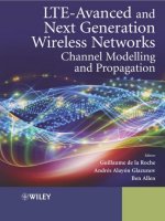
Figure 8.10 shows BER versus SNR for an STBC-CDMA system using OC codes with variable
numbers of transmitter antennae, from 2 up to 32 antennae. It illustrates that a great advantage can
be obtained by using a relatively large number of transmitter antennae. The results reveal that the
BER performance for an OC code STBC-CDMA system under the Rayleigh fading channels can
monotonously approach that of the single user noise only bound if a sufficiently large number of
antennae can be made available. Figure 8.10 gives purely theoretical results and deals with only the
OC codes.
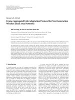
The comparison between STBC-CDMA systems under flat Rayleigh fading with different codes
is made in Figure 8.11, which shows the BER performance versus SNR for a system setup with two
transmitter antennae and one receiver antenna. The PG values are 31 and 63 for Gold codes, but
only 63 for M-sequence. In this figure, we do not give simulation results. It is seen from the figure
that an STBC-CDMA with the OC codes perform much better than that with either Gold codes or
M-sequences.
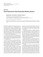
Figure 8.12 compares the BER results obtained from the theoretical analysis and computer simu-
lations for an STBC-CDMA system with either OC codes or M-sequences. The number of users in the
STBC-CDMA with M-sequences changes from 2, 4, and 8. It is not surprising that the STBC-CDMA
10
0
10
−5
10

−10
BER
10
−15
10
−20
Figure 8.10 BER versus signal-to-noise-ratio for an STBC-CDMA system in Rayleigh fading chan-
nels with a variable number of transmitter antennae. The performance is independent of the number
of users and PG values, showing the MAI-free property of the proposed system.
MIMO SYSTEMS 355
10
0
10
−1
10
−2
10
−3
10
−4
10
−5
10
−6
BER
Figure 8.11 The BER performance comparison under the Rayleigh fading channel for an STBC-
CDMA system using orthogonal complementary code, Gold codes (PG = 31 and 63) and M-sequence
(PG = 63), where eight users are present in the system. Only theoretical results are shown. Two
transmitter antennae and one receiver antenna are used.
OC theory

M-sequence 2 users theory
M-sequence 4 users theory
M-sequence 8 users theory
M
-sequence 2 users simulation
M
-sequence 4 users simulation
M
-sequence 8 users simulation
OC simulation
10
0
10
−1
10
−2
10
−3
10
−4
BER
10
−5
10
−6
Figure 8.12 BER performance comparison for an STBC-CDMA system with orthogonal complemen-
tary codes and M-sequences (PG = 63) with both theoretical analysis and computer simulation. A flat
Rayleigh fading channel is present and the number of users varies from 2, 4, and 8. Two transmitter
antennae and one receiver antenna are used.
356 MIMO SYSTEMS

10
0
10
−1
10
−2
10
−3
10
−4
BER
10
−5
10
−6
10
−7
Figure 8.13 Comparison of BER versus signal-to-noise-ratio for an OC STBC-CDMA and an STBC
Gold code DS-CDMA systems in Rayleigh fading channels with a variable number of users. The
PG for OC codes and Gold codes is 64 and 63 respectively. Two transmitter antennae and a single
receiver antenna are used.
10
0
10
−2
10
−4
10
−6
10

−8
BER
10
−10
10
−12
Figure 8.14 Comparison of BER versus signal-to-noise-ratio for STBC-CDMA and STBC Gold code
DS-CDMA systems in Rayleigh fading channels with a variable number of users. The PG for OC
codes and Gold codes is 64 and 63 respectively. Four transmitter antennae and a single receiver
antenna are used.
MIMO SYSTEMS 357
M
M
Figure 8.15 Capacity comparison for an STBC-CDMA system with orthogonal complementary codes,
Gold codes (PG = 31 and 63) and M-sequences (PG = 31 and 63). Two transmitter antennae and one
receiver antenna are used. The BER requirement is fixed at 0.001. A flat Rayleigh fading channel is
considered.
system with the M-sequences is very sensitive to the change in user population; while the system with
the OC codes offers a BER performance independent of user population, manifesting an MAI-free
operation. A very good match between the results obtained from analysis and simulation is also shown
in the figure. Similar conclusions can be made with respect to a system using other unitary codes.
Figures 8.13 and 8.14 compare the BER performance of an STBC-CDMA system with OC codes
and Gold codes (PG = 63). The two figures are obtained by using a similar system setup, except for
the difference in the number of transmitter antennae, being two in Figure 8.13 and four in Figure 8.14,
respectively. The number of users in the system with Gold codes varies from 2 to 64, demonstrating
how BER will change with the MAI level. It is clearly shown that the curve for the OC code behaves
like a single user bound for the curves obtained for Gold codes. A similar observation can also be
made from Figure 8.12, where an OC code is compared with M-sequences.
To explicitly show how much the difference in terms of capacity can be by using different
codes, Figures 8.15 and 8.16 are given, which basically concern a similar working environment,

except for the difference in the number of transmitter antennae, being two in Figure 8.15 and four in
Figure 8.16, respectively. Both the figures were obtained by fixing the BER at 0.001. Three different
codes are compared with one another, which are OC code, Gold codes with PG being 31 and 63, and
M-sequences with PG being 31 and 63.
The capacity advantage for an STBC-CDMA system based on an OC code over its counterpart,
either Gold codes or M-sequences, can be significant due to its interference-free operation. Assume,
for instance, that the required BER is about 10
−3
as specified in both the figures. It is observed
from Figure 8.16 that an OC code–based STBC-CDMA system with four antennae can support as
many as 64 users at SNR = 10.06, which is in fact limited only by the set size of the OC code
set (PG = 64). However, either a Gold code (PG = 63) or an M-sequence (PG = 63) STBC-CDMA
with four antennae can only support about 2 users, differing from that of the OC code STBC-CDMA
system by as many as 62 users! Alternatively, in order to achieve the same capacity, an unitary
code–based STBC-CDMA system has to use much more (which must be more than 32 antennae
358 MIMO SYSTEMS
M
M
Figure 8.16 Capacity comparison for an STBC-CDMA system with orthogonal complementary codes,
Gold codes (PG = 31 and 63) and M-sequences (PG = 31 and 63). The four transmitter antennae and
one receiver antenna are concerned. The BER requirement is fixed at 0.001. A flat Rayleigh fading
channel is considered.
10
0
10
−2
10
−4
10
−6

10
−8
10
−10
BER
Figure 8.17 BER comparison versus the number of users for an STBC-CDMA system under a
normalized three-path channel (whose delay profile is [
√
0.6,
√
0.3,
√
0.1]) with orthogonal comple-
mentary codes (PG = 8 ×8), Gold codes (PG = 63) and OVSF code (PG = 64). Two transmitter
antennae and one receiver antenna are concerned.
MIMO SYSTEMS 359
from our study) transmitter antennae at the same BER performance (10
−3
), thus definitely resulting
in much greater complexity.
Figure 8.17 shows the performance of an STBC-CDMA scheme using different CDMA codes
under a multipath channel with its delay profile being (
√
0.6,
√
0.3,
√
0.1). The three codes used here
are Gold code, OVSF code, and OC code with their PG values being 63, 64 and 8 ×8, respectively.
It is seen from the figure that the scheme with the OC code offers a superior BER performance under

various scenarios of user population in the system. The OVSF code performs worst and the Gold
code gives a slightly better BER than that of the OVSF code, but is never comparable to that of the
OC code.
We can summarize the results obtained so far regarding the OC codes–based STBC-CDMA
systems as follows. In these sections we have studied an STBC-CDMA system in downlink Rayleigh
fading channels. A comprehensive analysis has been carried out to derive the BER performance
expression of such a system under MAI and flat fading. It has been shown through the analysis that
an OC code–based STBC-CDMA system can achieve an ideal MAI-free operation and a full diversity
gain jointly under a single system framework. The results obtained from the theoretical study have
also been compared with those generated from computer simulations, and they have been shown to
match one another, for the most part. A unitary code–based STBC-CDMA still suffers serious MAI
problems even with the help of the full diversity gain of the STBC scheme. On the other hand, an
OC code STBC-CDMA system can offer a capacity limited only by noise and fading, and not by
interference. The results obtained here concluded that the integration of an OC code–based CDMA
and STBC system is technically feasible.

9
Cognitive Radio Technology
Cognitive radio (CR) is a newly emerging technology [789, 790], which has been recently proposed
to implement some kind of intelligence to allow a radio terminal to automatically sense, recognize,
and make wise use of any available radio frequency spectrum at a given time. The use of the available
frequency spectrum is purely on an opportunity driven basis. In other words, it can utilize any idle
spectrum sector for the exchange of information and stop using it the instant the primary user of the
spectrum sector needs to use it. Thus, cognitive radio is also sometimes called smart radio, frequency
agile radio, police radio,oradaptive software radio,
1
and so on. For the same reason, the cognitive
radio techniques can, in many cases, exempt licensed use of the spectrum that is otherwise not in use
or is lightly used; this is done without infringing upon the rights of licensed users or causing harmful
interference to licensed operations.

9.1 Why Cognitive Radio?
The discussion on cognitive radio technology can best begin with the remark made by Ed Thomas,
former Chief Engineer of the Federal Communication Commission (FCC). “If you look at the entire
radio frequency (RF) up to 100 GHz, and take a snapshot at any given time, you’ll see that only 5
to 10 % of it is being used. So there’s 90 GHz of available bandwidth.” This shows that the usage of
the radio spectrum is severely inefficient, and therefore the cognitive radio can be extremely useful
to exploit the unused spectrum from time to time, as long as the vacancy appears in the spectrum.
The radio spectrum, as regulated by the FCC in the United States (in a similar way in many other
countries also), is divided into channels which are usually licensed by individuals, corporations, and
municipalities as primary users. Most of these channels actively transmit only for the duration of a
small fraction of time. This is an inefficient use of the available spectrum. Clearly, if all those unused
spectra can be utilized, many more radio users can be accommodated without the need to create a
new spectrum.
Radio spectrum is one of the most important natural resources in the world today, and it is
necessary to build up a wireless information infrastructure. Insufficient radio spectrum has always
been a serious bottleneck for the deployment of a wireless information superhighway in the world. For
a long time, we have been resorting to three major strategies to accommodate growing radio/wireless
1
There is a difference between Software Definable Radio (SDR) and cognitive radio, which has to be explained
later. SDR has been discussed briefly in Section 6.1.5.
Next Generation Wireless Systems and Networks Hsiao-Hwa Chen and Mohsen Guizani
 2006 John Wiley & Sons, Ltd
362 COGNITIVE RADIO TECHNOLOGY
based applications. First of all, we have been trying hard to persuade existing radio spectrum owners
or licencees to vacate their legacy radio applications (for instance, the terrestrial microwave relay
trunk systems) to make way for the deployment of newly emerging wireless services, such as mobile
cellular networks, and so on. Nowadays, almost all (if not all) legacy radio users in most developed
countries who can possibly be reallocated have been moved away from the prime spectrum sectors
(roughly from 800 MHz to 5 GHz bands). Therefore, this strategy for spectrum clearance will be
of little help in solving the problem with severe spectrum shortage. The second traditional way of

accommodating new wireless applications is to move the carrier frequency to new high spectrum
sectors, which have been occupied by very few radio applications. Those new high radio spectra
includes millimeter waves from 10–30 GHz bandwidth. The positive aspect of using a relatively
high frequency spectrum is the ease with which broadband applications where very high data rates
can be implemented are supported. However, the shortcomings of using a very high carrier frequency
are obvious. One of the most problematic issues is that radio propagation properties in very high
frequency spectra are very sensitive to rain, dust, water vapor, and other small particles in the air. In
other words, the radio transmission in very high frequency ranges will no longer be weather-proof.
Therefore, the outage rate will become unacceptably high under rain, snow, and/or other weather
conditions. Finally, the third approach used to support more radio applications in an already crowded
spectrum is to overlay/underlay the new wireless applications on top of existing radio services.
The second generation mobile cellular standard, IS-95A/B, which works on direct-sequence CDMA
technology, was initially proposed for the work on the 900 MHz PCS spectrum in North America to
overlay many existing radio applications. The success of the overlay operation is largely based on
relatively low power spread spectrum transmissions from the CDMA technology. Another example
of such overlay applications is the ultra-wideband (UWB) technology, whose bandwidth overlaps
with those previously allocated for GPS, radar, and satellite services. Therefore, a strict low power
spectral density (PSD) emission mask is necessary to control the UWB transmission power level
below a certain threshold in order to not interfere with them.
It is obvious that all the above three major strategies to introduce new radio applications on top of
an already very crowded spectrum chart cannot solve the problem. Therefore, the need to search for
a more effective solution to solve the problems of severe spectrum shortage has become imperative.
Cognitive radio technology was introduced for this purpose.
To have a real picture of the current radio spectrum allocation situation, the readers may refer to
the US Frequency Allocation Chart [792] (in this chart, all radio spectrum allocations from 3 kHz up
to 300 GHz are shown), which is available from the web site of US National Telecommunications
and Information Administration. Similar situations can be found in many other developed countries,
such as Japan and in Europe. The US Frequency Allocation Chart is shown in Figure 9.1, which is
too large to show all spectrum allocation details clearly within a page. We use it here just to give
readers an idea of what it looks like.

The justification to use cognitive radio technology on top of the existing spectrum licencees to
provide various wireless applications on a licensed exempt basis can be summarized as follows.
Firstly and as discussed above, an unused spectrum is not desirable. Users should not be allowed
to own a spectrum that they do not use. It is also recommended that allocated spectra should not be
underutilized. Whatever the reasons for not fully using the allocated spectrum (economic, historic,
or other systemic reasons), it does not represent the best and highest use of this valuable and scarce
public resource.
Secondly, layering more licensed allocations on top of existing allocations as a solution to the
underutilized spectrum does not, in many people’s view, increase the economic incentives for new
applications in these spectrum slots, since obtaining investor support required to build licensed
services becomes problematic when the economic history of a particular allocation in a particular
geographic area has shown little promise for significant profits. On the other hand, licence exempt
use can support business models which do not require large capital investment to roll out services
because of the low cost of unlicensed equipment and the lack of the high up-front costs of acquiring
COGNITIVE RADIO TECHNOLOGY 363
Figure 9.1 US Frequency Allocation Chart [792] from 3 kHz up to 300 GHz. It should be noted that
a vacancy can only be found from 3 kHz to 9 kHz, which is shown in the left corner of the first row.
a spectrum at an auction (especially the case in the United States, Europe, and many other developed
countries). As a result, rural and other low population density areas could obtain services which would
otherwise be unavailable from the business entities which operate on licensed spectra and tend to
focus their investments on the larger, more profitable, urban and suburban marketplaces. For similar
reasons, community based networks and other not-for-profit groups could make use of otherwise
unused spectra to offer their constituencies innovative services and applications that would otherwise
be viewed as uneconomic, and, as a result, ignored by profit-oriented entities.
Thirdly, the assertions made by some people that licence exempt use interferes with business
opportunities flies in the face of the clear evidence that a vast amount of spectrum remains unused
because the high cost of rolling out licensed infrastructure is not justified on investment basis. Without
the opportunity to reclaim this spectrum in the public interest using cognitive radio technology under
licence exempt rules, this fallow spectrum would continue to be underutilized. In the broader context
of licence exempt sharing of licensed spectrum, it is widely believed that opportunities exist to apply

sophisticated cognitive radio technologies to recover otherwise underutilized spectrum for uses which
have significant economic and societal benefits without harming the interests of licensed services.
Finally, the current state-of-the-art radio technology has made it possible to implement a practical
cognitive radio in various wireless applications, such as wireless regional area networks (WRANs),
wireless metropolitan area networks (WMANs), wireless local area networks (WLANs), and wireless
personal area networks (WPANs), and so on, at a reasonable cost. Therefore, the radio terminals can be
given some intelligence to work automatically on the available frequency spectrum at any given time.
364 COGNITIVE RADIO TECHNOLOGY
In fact, a cognitive radio extends the functionality of a software-definable radio (SDR) to permit it to
react and adapt intelligently to its environment. It provides a central nervous system to communications
and computing platforms. This permits intelligent access and configuration by the radio devices.
9.2 History of Cognitive Radio
The cognitive radio is an emerging new technology, which is far from mature in terms of real applications
in current wireless systems and networks. Today, to implement a practical cognitive radio, many hurdles
should be overcome, and it is still too early to tell what a cognitive radio should look like for different
wireless applications. Therefore, the history of cognitive radio technology is still relatively short.
Mitola’s work
A comprehensive description of the term cognitive radio was first discussed in a paper written by J.
Mitola III and Gerald Q. Maguire in 1999 [793]. In 2000, J. Mitola III wrote his PhD dissertation
[794] on cognitive radio as a natural extension of the SDR concept. When addressing the broad
issue of wireless personal digital assistants (PDAs) in his dissertation, Mitola mentioned that the term
cognitive radio identifies the point at which wireless PDAs and the related networks are sufficiently
computationally intelligent regarding radio resources and related computer-to-computer communica-
tions to (a) detect user communications needs as a function of use context, and (b) to provide radio
resources and wireless services most appropriate to those needs.
FCC’s initiatives
In 2002, the FCC’s Spectrum Policy Task Force Report [797] identified that most spectra go unused
most of the time, as shown in Figure 9.2. Consequently, it was then realised that spectrum scarcity is
driven mainly by archaic systems for spectrum allocation and not by a fundamental lack of spectra.
Figure 9.2 A sample of the snapshot of radio spectrum utilization up to 6 GHz. It is shown that most

frequency bands were not used at the time when this snap shot was taken.
COGNITIVE RADIO TECHNOLOGY 365
How to open up additional spectra, whether it should be licensed or unlicensed, and the economic
implications of these decisions, have been topics of considerable debate [798]. Cognitive radio tech-
nology offers a possible solution based on a more sophisticated or intelligent system for allocating
spectra that can dramatically increase the amount of spectra available to network operators and indi-
vidual users. In particular, on December 20, 2002, it was stated in FCC’s “Notice of Inquiry” (NOI)
titled “Additional Spectrum for Unlicensed Devices Below 900 MHz and in the 3 GHz Band” (FCC-
02-328) that it opens the question of using fallow TV band channels for unlicensed services on a
noninterference basis. In the NOI, the FCC states that specifically, an unlicensed device should be
able to identify unused frequency bands before it can transmit, that is, by using Dynamic Frequency
Selection (DFS) and Incumbent Profile Detection (IPD) algorithms.
On November 13 of 2003, FCC issued NOI and “Notice of Proposed Rulemaking” (NPRM) titled
“Establishment of an Interference Temperature Metric ” (FCC-03-289), in which it proposed an
interference temperature model for quantifying and managing interference. The interference temper-
ature is calculated by T
int
=
N+I
kB
. It also stated that for an interference temperature limit to function
effectively on an adaptive or real-time basis, a system (cognitive radio) would be needed to measure,
and a response process would also be needed.
In another NPRM and order titled “Facilitating Opportunities for Flexible, Efficient, and Reliable
Spectrum Use Employing Cognitive Radio Technologies” (FCC-03-322), issued by FCC on December
17, 2003, it was stated that a wide ranging NPRM exploring a broad range of issues related to cognitive
radio technology will be required. It pointed out that the FCC wants to push for advances in technology
which support more effective spectrum use. Among these advances are cognitive radio technologies
that can possibly make more intensive and efficient spectrum use by licencees within their own
networks, and by spectrum users sharing spectrum access on a negotiated or an opportunistic basis.

The FCC’s action sparked a lot of response from both industry and academia, and some research
activities on cognitive radio [798–801] in the last few years. However, the most important event in
the development of cognitive radio happened in 2004, when the FCC issued yet another NPRM that
raised the possibility of permitting unlicensed users to temporarily “borrow” spectrum from licensed
holders as long as no excessive interference was seen by the primary user [795]. Devices that borrow
spectrum on a temporary basis without generating harmful interference are commonly referred to as
“cognitive radios” [796]. Basic cognitive radio techniques, such as DFS and transmit power control
(TPC), already exist in many unlicensed devices. However, to make a practical cognitive radio termi-
nal, we have to deal with many serious challenges.
The FCC is proposing specific rulemaking in the unlicensed arena related to cognitive technology
as follows:
• Opening three new bands to unlicensed operation based on DFS and TPC protocols (inter-
ference temperature NPRM), which include 6525–6700 MHz (175 MHz), 12.75–13.15 GHz
(400 MHz), and 13.2125–13.25 GHz (37.5 MHz);
• Allowing six times more transmitter power for cognitive radio devices (under Part 15.247 and
Part 15.249) where the ISM band is lightly used (cognitive radio NPRM);
• DFS thresholds at which frequency change is required: For Tx power levels < 23 dBm:
−62 dBm; For Tx power levels > 23 dBm: −64 dBm; DFS threshold averaging time varies
with rule: unlicensed national information infrastructure (U-NII) is 1 µs, new interference tem-
perature bands: 1 ms; DFS thresholds are referenced to the output of an omni-directional
antenna.
• The definition of an unoccupied band: RSL < −83 dBm measured in a 1.25 MHz bandwidth
using an omni-antenna.
• Minimum TPC backoff from maximum allowed Tx power: −6 dB, triggered by a vendor
specific criterion for link quality.
366 COGNITIVE RADIO TECHNOLOGY
Related IEEE standards
On the other hand, the standardization work done by the Institute of Electrical and Electronics
Engineers (IEEE) has also been carried out parallel to the FCC’s action. Recent IEEE 802 standards
activity in cognitive radio includes a recently approved amendment to the IEEE 802.11 operation, or

the IEEE 802.11h, which incorporates DFS and TPC protocols for 5-GHz operations under the IEEE
802.11a standard [449–451].
Because 802.11a wireless networks operate in the 5-GHz radio frequency band and support as
many as 24 nonoverlapping channels, they are less susceptible to interference than their 802.11b/g
counterparts. However, regulatory requirements governing the use of the 5-GHz band vary from
country to country, hampering 802.11a deployment. In response, the International Telecommunication
Union (ITU) recommended a harmonized set of rules for WLANs to share the 5-GHz spectrum
with primary-use devices such as military radar systems. Approved in September 2004, the IEEE
802.11h standard defines mechanisms that 802.11a WLAN devices can use to comply with the ITU
recommendations. These mechanisms are DFS and TPC. WLAN products supporting 802.11h have
already been available in the second half of 2005. DFS detects other devices using the same radio
channel, and it switches the WLAN operation to another channel if necessary. DFS is responsible for
avoiding interference with other devices, such as radar systems and other WLAN segments, and for
uniform utilization of channels.
Among other activities carried out by the IEEE is 802.18 SG1, which was established at the
Albuquerque Plenary in November 2003, and focused on creating the following: (1) Recommenda-
tions for a rule making proposal to the FCC on TV band use by unlicensed devices. (2) A Project
Authorization Request (PAR) and associated five Criteria documents to create a network standard
aimed at unlicensed operation in the TV band. In “Reply to Comments of IEEE 802.18” prepared by
Carl R. Stevenson () in May 2004, it indicated clearly that IEEE 802.18 sup-
ports the opportunistic use of fallow spectrum by licence exempt networks on a noninterfering basis
with licensed services using cognitive radio techniques. IEEE 802.18 supports the FCC’s approach
to rural applications of cognitive radio technology as a means to increase the coverage area of wisps
and other unlicensed services in the ISM bands.
Earlier similar works
It has to be noted that, although the terminology of “cognitive radio” was only proposed recently,
the concept of intelligent radio is not completely new. Many previously carried out researches on
wireless communications and networks bear some similarity to what a cognitive radio does. The
first example of such research is the collision avoidance protocol used in IEEE 802.3 standard or
Ethernet standard: carrier sense multiple access (CSMA).

2
The basic idea for CSMA is to sense
before transmitting, which works in a very similar way to what a cognitive radio unerringly does.
This polite radio transmission etiquette forms the core of today’s cognitive radio technology.
Another example of similar research is the so-called “dynamic channel selection/allocation,”
which has been extensively used in user traffic channel assignment schemes in mobile cellular systems.
A new mobile terminal will be assigned a traffic channel with an available idle channel from the
traffic channel pool. Its utilization will be released back to the pool when its transmission ends, thus
making it available to others’ use. Naturally, the intelligence level possessed in a cognitive radio will
be much higher than that available in all previous wireless applications.
9.3 What is Cognitive Radio?
In this section, we define cognitive radio and investigate the algorithms and types of technologies
that already exist.
2
CSMA has been discussed in Section 2.3.4 of this book.
COGNITIVE RADIO TECHNOLOGY 367
9.3.1 Definitions of Cognitive Radio
As any newly emerging technology, the definition of “cognitive radio” can be seen in many dif-
ferent ways. In fact, the term Cognitive Radio means different things to different audiences. The
earlier definition by Joseph Mitola in his dissertation titled “Cognitive Radio – An Integrated Agent
Architecture for Software Defined Radio” [794], was given as follows. The cognitive radio iden-
tifies the point at which wireless PDAs and the related networks are sufficiently computationally
intelligent on the subject of radio resources and related computer-to-computer communications to (a)
detect user communications needs as a function of use context, and (b) to provide radio resources
and wireless services most appropriate to those needs. Cognitive radio increases the awareness that
computational entities in radios have of their locations, users, networks, and the larger environ-
ment. Mitola included the concept of machine learning as a property of cognitive radio. Mitola’s
definition on cognitive radio includes a high level of awareness and autonomy, in a sense that cog-
nition tasks, that might be performed, range in difficulty from the goal driven choice of RF band,
air interface, or protocol to higher-level tasks of planning, learning, and evolving new upper layer

protocols.
The FCC gave the following definition on cognitive radio [795]. A cognitive radio is a radio that
can change its transmitter parameters based on interaction with the environment in which it operates.
At the same time, it should also note that FCC refers to a SDR as a transmitter in which the operating
parameters can be altered by making a change in software that controls the operation of the device
without changes in the hardware components that affect the radio frequency emissions. It went on
to claim that the majority of cognitive radios will probably be SDRs, but neither having software nor
being field reprogrammable are requirements of a cognitive radio.
To summarize from the aforementioned two versions of definitions on cognitive radio, we can
see that Mitola emphasized the level of device/network intelligence which adapts to user activity;
while the FCC seems primarily concerned with a regulatory friendly view, focused on transmitter
behavior at the moment. Therefore, the relationship between the cognitive radio and SDR from
the views of Mitola and the FCC can be seen in Figure 9.3, where cognitive radio adapts to the
spectrum environment; while SDR adapts to the network environment. They partially overlap in their
functionalities.
9.3.2 Basic Cognitive Algorithms
It is therefore not difficult to discern that a fully functional cognitive radio should have the ability to
do the following works: (1) Tune to any available channel in the target band. (2) Establish network
communications and operate in all or part of the channel. (3) Implement channel sharing and power
Figure 9.3 The cognitive radio adapts to the spectrum environment; while SDR adapts to the network
environment. Their functionalities are partially overlapped.
368 COGNITIVE RADIO TECHNOLOGY
control protocols which adapt to spectra occupied by multiple heterogeneous networks. (4) Implement
adaptive transmission bandwidths, data rates, and error correction schemes to obtain the best through-
put possible. (5) Implement adaptive antenna steering to focus transmitter power in the direction
required to optimize received signal strength.
The core of a cognitive radio is its inherent intelligence, which makes it different from any normal
wireless terminal available today, in either 2- or 3G systems. This intelligence will allow a cognitive
radio to scan all possible frequency spectra before it makes an intelligent decision on how and when
to make use of a particular sector of the spectrum for communications. Therefore, it is inevitable

that a cognitive radio needs great signal processing power to deal with the vast amounts of data it
captures from various radio channels. Thus, the capability to process all those enormous amounts of
data on a real-time or quasi-real-time basis is a must for any cognitive radio.
It is still too early to specify exactly the algorithms that a cognitive radio should use at the moment
of writing this book. However, we would like to provide some evidence as to how a primitive cognitive
radio may behave. Obviously, any cognitive radio has to use the following two protocols for its very
basic operation: (1) DFS, and (2) TPC.
The DFS was originally used to describe a technique to avoid radar signals by 802.11a networks
which operate in the 5 GHz U-NII band. Now, it has been generalized to refer to an automatic
frequency selection process intended to achieve some specific objective (like avoiding harmful inter-
ference to a radio system with a higher regulatory priority). On the other hand, TPC was originally
a mechanism for 802.11a networks to lower aggregate transmit power by 3 dB from the maximum
regulatory limit to protect Earth Exploration Satellite Systems (EESS) operations. Now it has been
generalized to a mechanism that adaptively sets transmit power based on the spectrum or regulatory
environment. These two protocols will become a must for all cognitive radios.
In addition, a cognitive radio should have IPD capability [799], which is another key cognitive
radio behavior. The IPD is the ability to detect an incumbent user (one with regulatory priority)
based on a specific spectrum signature. The operation of IPD bears the following characteristics: (1)
DFS requires an IPD protocol to identify unoccupied, or lightly used frequencies. (2) IPD includes
detection schemes focused on the characteristics of the specific incumbents in the band, or bands, that
the cognitive radio is designed to support. (3) IPD eliminates the need for geo-location techniques
(GPS, etc.) to determine the location of the radio and, using a database, identifies unused channels.
As both TPC and IPD algorithms are intuitive, as suggested by its name, we will only explain
the implementation of the DFS cognitive algorithms in depth, in the following text.
The DFS algorithm was originally proposed in the ITU-R recommendation M.1461 [807] to avoid
possible interference to existing radar operations in the vicinity. Many radar systems and unlicensed
devices operating co-channels in proximity could produce a scenario where mutual interference is
experienced. The DFS methodology is used to compute the received interference power levels at
the radar and unlicensed device receivers. A DFS algorithm may provide a means of mitigating this
interference by causing the unlicensed devices to migrate to another channel once a radar system

has been detected on the currently active channel. This model first considers the interference caused
by the radar to the unlicensed device at the output of the unlicensed device antenna. If the received
interference power level at the output of the unlicensed device antenna exceeds the DFS detection
threshold, the unlicensed device will cease transmissions and move to another channel. The algorithm
then computes the aggregate interference to the radar from the remaining unlicensed devices. Each of
the technical parameters used in the method and the radar interference criteria will also be described.
The received signal level from the radar at the output of the unlicensed device antenna can be
evaluated by using the following equation:
I
U
= P
Radar
+ G
Radar
+ G
U
− L
Radar
− L
U
− L
P
− L
L
− FDR (9.1)
where I
U
is the received interference power at the output of the unlicensed device antenna in dBm,
P
Radar

is the peak power of the radar in dBm, G
Radar
is the antenna gain of the radar in the direction
COGNITIVE RADIO TECHNOLOGY 369
of the unlicensed device in dBi, G
U
is the antenna gain of the unlicensed device in the direction of
the radar in dBi, L
Radar
is the radar transmit insertion loss in dB, L
U
is the unlicensed device receive
insertion loss in dB, L
P
is the propagation loss in dB, L
L
is the building and nonspecific terrain
losses in dB, and FDR is the frequency dependent rejection in dB.
Equation (9.1) is calculated for each unlicensed device in the distribution. The value obtained is
then compared to the DFS detection threshold under investigation. Any unlicensed device for which
the threshold has been exceeded will begin to move to another channel, and consequently is not
considered in the calculation of interference to the radar, as given by
I
RADAR
= P
U
+ G
U
+ G
Radar

− L
U
− L
Radar
− L
P
− L
L
− FDR (9.2)
where I
RADAR
is the received interference power at the input of the radar receiver in dBm, P
U
is
the power of the unlicensed device in dBm, G
U
is the antenna gain of the unlicensed device in the
direction of the radar in dBi, G
Radar
is the antenna gain of the radar in the direction of the unlicensed
device in dBi, L
U
is the unlicensed device transmit insertion loss in dB, L
Radar
is the radar receive
insertion loss in dB, L
P
is the radio-wave propagation loss in dB, L
L
is the building and nonspecific

terrain losses in dB, and FDR is the frequency dependent rejection in dB.
With the help of equation (9.2), we can calculate each unlicensed device being considered in the
analysis that has not detected energy from the radar in excess of the DFS detection threshold. These
values are then used in the calculation of the aggregate interference to the radar by the unlicensed
devices using the following equation:
I
AGG
=
N

j =1
I
RADAR
j
(9.3)
where I
AGG
is the aggregate interference to the radar from the unlicensed devices in Watts, N is the
number of unlicensed devices remaining in the simulation, and I
RADAR
is the interference caused to
the radar from an individual unlicensed device in Watts.
It is necessary to convert the interference power calculated in Equation (9.2) from dBm to Watts
before calculating the aggregate interference seen by the radar using Equation (9.3).
The parameters used in the above DFS algorithm can be explained as follows: To obtain “radar
antenna gain” (G
Radar
), we need to know the azimuth and elevation antenna pattern models for the
radar considered. The models should provide the antenna gain as a function of an off-axis angle
for a given main beam antenna gain. The unlicensed device power level (P

U
) in this analysis is
assumed to be 38 dBm and 6.6 dBm. The building and nonspecific terrain losses (L
L
) include build-
ing blockage, terrain features, and multipath. In the above analysis, this loss has been treated as a
uniformly distributed random variable between 1 and 10 dB for each radar unlicensed device path.
When determining Radar and Unlicensed Device Transmit and Receive Insertion Losses (L
Radar
and
L
U
), we have assumed that the analysis includes a nominal 2 dB for the insertion losses between
the transmitter and receiver antenna and the transmitter and receiver inputs for the radar and the
unlicensed device. Finally, to compute the radio-wave propagation loss (L
P
), the NTIA Institute
for Telecommunication Sciences Irregular Terrain Model (ITM) was used [808]. The ITM model
computes radio-wave propagation based on the electromagnetic theory and on the statistical analysis
of both terrain features and radio measurements to predict the median attenuation as a function of
distance and variability of the signal in time and space.
9.3.3 Conceptual Classifications of Cognitive Radios
The characteristic features of a cognitive radio have a lot to do with the spectrum facts in different
regions or countries. If we are only looking at the US market, we will see that a lot of spectra have
been assigned for licensed use by the FCC. Actual spectrum use varies dramatically from region to
370 COGNITIVE RADIO TECHNOLOGY
region: spectrum is more congested in urban areas, and hardly used in rural areas. Some licensed
services only operate in a few locations nationally (for example, Fixed Satellite Services). Even in
urban areas, only a fraction of available spectra is in continuous use. We have to admit that, in terms
of reclaiming fallow spectrum, a lot of low hanging fruit is available for harvest using cognitive

techniques. Regulatory activity is just beginning to open up opportunities to reclaim lightly used
spectra for new services.
Currently, there are two conceptual forms of cognitive radios. One is called full cognitive radio,
in which every possible parameter observed by the wireless node and/or the network is taken into
account while making a decision on the transmission and/or reception parameter change. The other is
called Spectrum Sensing Cognitive Radio, which is a special case of Full Cognitive Radio in which
only the RF spectrum is observed.
Also, depending on the parts of the spectrum available for cognitive radio, we can distinguish
“Licensed Band Cognitive Radio” and “Unlicensed Band Cognitive Radio.” When a cognitive radio
is capable of using bands assigned to licensed users, apart from the utilization of unlicensed bands
such as the U-NII band or the ISM band, it is called a Licensed Band Cognitive Radio. One of the
Licensed Band Cognitive Radio-like systems is the IEEE 802.15 Task group 2 [802] specification.
On the other hand, if a cognitive radio can only utilize the unlicensed parts of a RF spectrum, it is
an Unlicensed Band Cognitive Radio. An example of an Unlicensed Band Cognitive Radio is IEEE
802.19 [803].
Although cognitive radio was initially thought of as an SDR extension (Full Cognitive Radio),
most of the current research work is focused on Spectrum Sensing Cognitive Radio, particularly on
the utilization of TV bands for communication. The essential problem of Spectrum Sensing Cognitive
Radio is the design of high-quality spectrum sensing devices and algorithms for exchanging spectrum
sensing data between different nodes in a cognitive radio network. It has been shown in [804] that
a simple energy detector cannot guarantee the accurate detection of signal presence. This calls for
more sophisticated spectrum sensing techniques and requires that information about spectrum sensing
must be regularly exchanged between nodes. In [805], the authors showed that the increasing number
of cooperating sensing nodes decreases the probability of false detection. To adaptively fill free RF
bands, OFDM seems to be a perfect candidate. Indeed in [801] T. A. Weiss and F. K. Jondral
from the University of Karlsruhe, Germany, proposed a Spectrum Pooling system in which free
bands sensed by nodes were immediately filled by OFDM subbands. Some of the applications of
Spectrum Sensing Cognitive Radio include emergency networks and WLAN higher throughput, and
transmission distance extensions.
9.4 From SDR to Cognitive Radio

SDR has now been widely accepted as the implement of choice for a variety of platforms and
applications. The success in harnessing the promised flexibility and incredible processing power of
the SDR has led designers to consider implementing cognitive radios that adapt to their environment
by analyzing the RF environment and adjusting the spectrum use appropriately. The key components
for the successful implementation of cognitive radio are low latency and adaptability to the operating
conditions. These are the essential characteristic features that are needed for the deployment of
cognitive radios in multiservice scenarios such as communications, electronic warfare (EW), and
radar. Cognitive radios thus represent a huge evolution of SDRs.
Therefore, the cognitive radio has a lot to do with SDR [789–791]. As a matter of fact, the cogni-
tive radio works largely on the basis of many functionalities of SDR.
3
It is of imperative importance
for us to understand how a software definable radio works in order to gain a better understanding of
cognitive radio. The discussion on SDR is to be covered in the subsection that follows.
3
A very brief introduction on SDR is also available in 6.1.5.
COGNITIVE RADIO TECHNOLOGY 371
9.4.1 How Does SDR Work?
An SDR is a collection of hardware and software technologies that enable reconfigurable system
architectures for wireless networks and user terminals. It provides an efficient and comparatively
inexpensive solution to the problem of building multimode, multiband, and multifunction wireless
devices that are able to work adaptively in a complex radio environment. In an SDR, all functions,
operation modes, and applications can be configured and reconfigured by various software. If the
configuration automation can be implemented in an SDR, a primitive cognitive radio will result.
The fundamental idea of SDR is to sample the received signal in the RF band right after the RF
low noise amplifier. It is also noted that the most important part of an SDR is its receiver part, rather
than its transmitter part. The reason is simple: the major difference between a conventional radio and
an SDR lies mainly in their methods of recovering required signals. Therefore, in this subsection we
will concentrate on the discussions on the SDR receiver.
The best way to describe what an SDR system looks like is to compare it with a traditional

heterodyne radio, as shown in Figure 9.4, which consists of a bandpass filter (BPF), a low noise
amplifier (LNA), a mixer, a frequency synthesizer, an intermediate frequency (IF) amplifier, an
automatic gain controller (AGC), a demodulator, an analog to digital converter (ADC), and a digital
signal processor (DSP), and so on. It is noted that filtering, amplification, and carrier down conversion
are implemented by analogue circuits. There might be several stages of IF amplification, thus needing
several IF filters, which makes it very difficult to miniaturize the terminal design due to their bulky
sizes.
On the contrary, in an ideal SDR receiver, as shown in Figure 9.5, the signal captured from a
wideband antenna will be directly sampled and analogue-to-digital converted; thus all postantenna
signal processing will be carried out in the digital domain. Therefore, the physical layer (PHY) air
interface signaling format will be determined “over the air,” or controlled by either a network or
a terminal operator. This feature is critical for the implementation of a cognitive radio. The only
difference is that a cognitive radio needs to scan a wide range of frequency spectra before deciding
which band to use, instead of a predefined one, as an SDR terminal does.
One of the most important characteristic features of an SDR terminal is that its signal is processed
almost completely in the digital domain, needing very little analogue circuit. This brings a tremendous
benefit to make the terminal very flexible (for a multimode terminal) and ultrasmall size with the
help of state-of-the-art microelectronics technology.
To implement an SDR receiver as shown in Figure 9.5, we have to raise the sampling frequency
up to at least twice as high as the carrier frequency seen from the antenna. For instance, if we are
interested in receiving the signals in a 10 GHz band, an ADC with a sampling rate of at least 20 Giga
samples per second has to be used. This will pose an even higher challenge if a cognitive radio needs to
scan an entire frequency spectrum up to millimeter bands. A compromise is to retain the RF front-end
Antenna
BPF BPFLNA Mixer
IF amplifiers
Demod ADC
I
Q
DSP

Output format
Synthesizer
Figure 9.4 A traditional heterodyne radio receiver structure used in a GSM terminal.
372 COGNITIVE RADIO TECHNOLOGY
RF
ADC DSP Decode
Audio
Video
Data
Figure 9.5 A generic SDR receiver structure, which directly samples signals in the RF band.
RF
RF front end
and down-
conversion
IF
ADC DSP
DSP
DSP
Output Format
Digital data bus
Figure 9.6 An SDR receiver structure with IF sampling implementation.
IF amplifier, and the signal will be sampled only at the IF bands, which will be much lower than RF
bands of interest and an ADC with a fixed sampling rate can be applied to all RF signals if the IF is
fixed. This can greatly simplify the architecture of an SDR receiver and lower the implementation cost.
An SDR receiver with IF sampling is shown in Figure 9.6, where different DSP chips will be used for
decoding different pay-loads carried in the RF signals.
9.4.2 Digital Down Converter (DDC)
An SDR terminal should be able to work under different air interface standards/modes. As mentioned
earlier, this requires that the signal be digitized as early as possible at a receiver, preferably right
after the antenna’s front end. However, the complexity of implementing direct RF sampling can be

formidable, so that the compromise that uses IF sampling is usually an attractive solution.
However, the use of the IF sampling technique gives rise to a new problem where the DSP
bandwidth and processing speed sometimes do not match the output signal from the ADC placed
after the IF amplifiers. Therefore, it is commonplace to use a digital down converter (DDC) to bridge
the gap between the DSP and the ADC output signal. The block diagram for the DDC is shown in
Figure 9.7, where signal processing algorithms can be explained by the following analysis.
First, the input wideband signal should be converted into complex baseband signal as
x
[
n
]
= r
[
n
]
e
−j 2πf
c
nT
s
= r
[
n
]
{
cos
(
2πf
c
nT

s
)
− j sin
(
2πf
c
nT
s
)
}
(9.4)
where r[n] is the sampled IF signal, f
c
is the carrier frequency, and T
s
is the sampling interval.
Now, this complex baseband signal is fed into an M-stage finite impulse response (FIR) filter, whose