Operational Risk Modeling Analytics phần 8 docx
Bạn đang xem bản rút gọn của tài liệu. Xem và tải ngay bản đầy đủ của tài liệu tại đây (2.29 MB, 46 trang )
BAYESIAN ESTIMATION
305
As
before, the parameter
6
may be scalar or vector valued. Determination
of the prior distribution has always been one of the barriers to the widespread
acceptance of Bayesian methods. It is almost certainly the case that your
experience has provided some insights about possible parameter values before
the first data point has been observed. (If you have no such opinions, perhaps
the wisdom of the person who assigned this task to you should be questioned.)
The difficulty is translating this knowledge into a probability distribution. An
excellent discussion about prior distributions and the foundations of Bayesian
analysis can be found in Lindley
[76],
and for a discussion about issues sur-
rounding the choice of Bayesian versus frequentist methods, see Efron
[26].
A
good source for
a
thorough mathematical treatment of Bayesian methods
is the text by Berger
[15].
In recent years many advancements in Bayesian
calculations have occurred.
A
good resource is
[21].
The paper by Scollnik
??
addresses
loss
distribution modeling using Bayesian software tools.
Because of the difficulty of finding
a
prior distribution that is convincing
(you will have to convince others that your prior opinions are valid) and the
possibility that you may really have no prior opinion, the definition of prior
distribution can be loosened.
Definition
10.21
An
improper prior distribution
is one for which the
probabilities (or pdf) are nonnegative
but
their sum (or integral)
is
infinite.
A great deal of research has gone into the determination of a so-called
noninformative
or
vague
prior. Its purpose is to reflect minimal knowledge.
Universal agreement on the best way to construct
a
vague prior does not exist.
However, there is agreement that the appropriate noninformative prior for
a
scale parameter is
~(6)
=
l/6,
6
>
0.
Note that this
is
an improper prior.
For
a
Bayesian analysis, the model is no different than before.
Definition
10.22
The
model distribution
is the probability distribution for
the data as collected giiien a particular value for the parameter. Its pdf is
denoted
fXp(xlO),
where vector notation for
x
is used to remind
us
that all
the data appear here. Also note that this
is
identical to the likelihood function
and
so
that name may
also
be used at tames.
If
the vector of observations
x
=
(XI,.
.
.
,
x,)~
consists of independent and
identically distributed random variables, then
We use concepts from multivariate statistics to obtain two more definitions.
In both cases,
as
well
as
in the following, integrals should be replaced by sums
if the distributions are discrete.
Definition
10.23
The
joint distribution
has pdf
306
PARAMETER ESTIMATION
Definition
10.24
The
marginal distribution
of
x
has pdf
Compare this definition to that of a mixture distribution given by formula
(4.5)
on page
88.
The final two quantities of interest are the following.
Definition
10.25
The
posterior distribution
is the conditional probability
distribution
of
the parameters given the observed data. It is denoted
.iro~~(Oix).
Definition
10.26
The
predictive distribution
is the conditional proba-
bility
distribution
of
a new observation y given the data
x.
It
is denoted
fulx(Ylx).g
These last two items
are
the key output of
a
Bayesian analysis. The pos-
terior distribution tells us
how
our opinion about the parameter has changed
once we have observed the data. The predictive distribution tells us what
the next observation might
look
like given the information contained in the
data
(as
well as, implicitly, our prior opinion). Bayes’ theorem tells us how
to compute the posterior distribution.
Theorem
10.27
The posterior distribution can be computed
as
(10.2)
while the predictive distribution can
be
computed as
~YIX(Y~X)
=
/
fuio(dQ)~oix(Qlx)
do,
(10.3)
where fulo(ylQ) is the pdf
of
the new observation, given the parameter value.
The predictive distribution can be interpreted as a mixture distribution
where the mixing is with respect to the posterior distribution. Example
10.28
illustrates the above definitions and results.
Example
10.28
Consider the following losses:
125 132 141 107
133
319 126 104 145 223
this section and in any subsequent Bayesian discussions,
we
reserve
f(.)
for distribu-
tions concerning observations (such
as
the model and predictive distributions) and
K(.)
for
distributions concerning parameters (such
as
the prior and posterior distributions). The
arguments will
usually
make it clear which particular distribution is being used.
To
make
matters explicit, we
also
employ subscripts to enable
us
to keep track
of
the random vari-
ables.
BAYESlA
N
ES
TI
MA
TI0
N
30
7
The amount
of
a single
loss
has the single-parameter Pareto distribution with
6
=
100 and
cu
unknown. The prior distribution has the gamma distribution
with
cu
=
2
and
6
=
1. Determine all
of
the relevant Bayesian quantities.
The prior density has
a
gamma distribution and is
~(a)
=
ae-a,
a
>
0,
while the model is (evaluated
at
the data points)
10
-3.801121a-49.852823
=a
e
ay
100)10*
fXiA(xlQ)
=
The joint density of
x
and
A
is (again evaluated at the data points)
11
-4.801121a-49.852823
fX,A(X,
a)
=
a
e
The posterior distribution of
a
is
cu11e-4.801121a-49.852823
alle-4.801121a
- -
(10.4)
There is no need to evaluate the integral in the denominator. Because we
know that the result must be a probability distribution, the denominator is
just the appropriate normalizing constant.
A
look at the numerator reveals
that we have a gamma distribution with
cu
=
12
and
9
=
1/4.801121.
xAIx(cuIx)
=
cu11e-4.801121a-49.852823
,-ja
(11!)(1/4301121)12'
The predictive distribution
is
00
a,OOa
alle-4.801121a
dcu
fyix(y'x)
=
Jo'
7
(11!)(1/4.801121)12
00
-
1 cu12e-(0.195951+ln
9)"
da
y(
11!)( 1/4.801121)12
Jo'
-
-
1
(12!)
-
y(11!)(1/4.801121)12 (0.195951
+
lny)13
y
>
100.
12( 4.801 121)
l2
~(0.195951
+
lny)I3'
-
-
(10.5)
While this density function may not look familiar, you are asked to show in
Exercise
10.43
that 1nY
-
In
100
has the Pareto distribution.
10.5.2
Inference and prediction
In one sense the analysis
is
complete. We begin with
a
distribution that
quantifies our knowledge about the parameter and/or the next observation
and we end with
a
revised distribution. However, you will likely want to
308
PARAMETER EST/MAT/ON
produce a single number, perhaps with a margin for error, is what is desired.
The usual Bayesian solution is to pose a loss function.
Definition
10.29
A
loss
function
lj(6j,6j)
describes the penalty paid
by
the investigator when
8,
is
the estimate and
6,
is the true value
of
the jth
parameter.
It is also possible to have
a
multidimensional loss function
l(&
0)
that allows
the
loss
to depend simultaneously on the errors in the various parameter
estimates.
Definition 10.30
The
Bayes estimator
for a given
loss
function is the
estimator that minimizes the expected
loss
given the posterior distribution
of
the parameter
in
question.
The three most commonly used
loss
functions are defined
as
follows.
Definition 10.31
For
squared-error
loss
the
loss
function
is
(all subscripts
are dropped for convenience) l(6,6)
=
(6
-
6)2.
For
absolute
loss
it is
l(6,O)
=
16
-
61.
For
zero-one
loss
it
is
l(6,6)
=
0
if
6
=
6
and is
1
otherwise.
Theorem 10.32 indicates the Bayes estimates for these three common loss
functions.
Theorem 10.32
For squared-error
loss,
the Bayes estimator
is
the mean
of
the posterior distribution, for absolute
loss
it is a median, and for zero-one
loss
it
is
a mode.
Note that there is
no
guarantee that the posterior mean exists
or
that the
posterior median
or
mode will be unique. When not otherwise specified, the
term
Bayes estimator
will refer to the posterior mean.
Example 10.33
(Example 10.28 continued)
Determine the three Bayes esti-
mates
of
a.
The mean of the posterior gamma distribution is
a6
=
12/4.801121
=
2.499416. The median of 2.430342 must be determined numerically while the
mode is
(a
-
1)6
=
11/4.801121
=
2.291132.
Note that the
CY
used here is
the parameter of the posterior gamma distribution, not the
CY
for the single-
0
parameter Pareto distribution that we are trying to estimate.
For
forecasting purposes, the expected value
of
the predictive distribution
is often of interest.
It
can be thought of
as
providing a point estimate of the
(n+
1)th observation given the first
n
observations and the prior distribution.
BAYESIAN ESTIMATION
309
It is
J
Equation
(10.6)
can be
distribution
as
weights.
(10.6)
interpreted as a weighted average using the posterior
Example
10.34
(Example
10.28
continued)
Determine the expected value
of
the 11th observation, given the first 10.
For
the single-parameter Pareto distribution, E(Y/a)
=
100a/(a
-
1)
for
a
>
1.
Because the posterior distribution assigns positive probability to values
of
a
5
1,
the expected value of the predictive distribution is not defined.
I7
The Bayesian equivalent of
a
confidence interval is easy to construct. The
following definition will suffice.
Definition
10.35
The points
a
<
b
define a lOO(1-
a)%
credibility inter-
val
for
0,
provided that
Pr(a
<
Oj
5
bjx)
>
1
-
a.
The inequality is present for the case where the posterior distribution
of
0,
is discrete. Then it may not be possible for the probability to be exactly
1
-
a.
This definition does not produce a unique solution. Theorem 10.36
indicates one way to produce
a
unique interval.
Theorem
10.36
If
the posterior random variable
Bjlx
is continuous and uni-
modal, then the lOO(1
-
a)%
credibility interval with smallest width
b
-
a
is
the unique solution to
~b7r~3~x(Bjjx)dBj
=
1
-a,
"qx(al4
=
"o~x(w.
This interval is
a
special case
of
a highest posterior density (HPD) credibility
set.
Example 10.37 may clarify the theorem.
Example
10.37
(Example
10.28
continued)
Determine the shortest
95%
credibility interval for the parameter
a.
Also
determine the interval that places
2.5% probability at each end.
310
PARAMETER ESTIMATION
07
~
06
05
-
-
-I
-~
~~
-Equalprobability
interval
p
04
02
0
1
2
3
4
5
+
Fig.
10.1
Two
Bayesian credibility intervals
The two equations from Theorem
10.36
are
Pr(a
5
A
5
blx)
=
r(12;4.801121b)
-
r(12;4.801121~)
=
0.95,
a11e-4.801121a
=
b11e-4.801121b
7
and numerical methods can be used to find the solution
a
=
1.1832
and
b
=
3.9384.
The width of this interval is
2.7552.
Placing
2.5%
probability at each end yields the two equations
r(12; 4.801121b)
=
0.975,
r(12; 4.801121~)
=
0.025.
This solution requires either access to the inverse of the incomplete gamma
function
or
the use of root-finding techniques with the incomplete gamma
function itself. The solution is
a
=
1.2915
and
b
=
4.0995.
The width is
2.8080,
wider than the first interval. Figure
10.1
shows the difference in the
two intervals. The solid vertical bars represent the HPD interval. The total
area to the left and right of these bars is
0.05.
Any other
95%
interval must
also have this probability. To create the interval with
0.025
probability on each
side, both bars must be moved to the right.
To
subtract the same probability
on the right end that is added on the left end, the right limit must be moved
a
greater distance because the posterior density is lower over that interval than
it is on the left end. This must lead to
a
wider interval.
Definition
10.38
provides the equivalent result for any posterior distribu-
tion.
Definition
10.38
For
any posterior distribution the 100(1-a)%
HPD
cred-
ibility set
is
the set
of
parameter values
C
such
that
Pr(Bj
E
C)
2
1
-
Q
(10.7)
and
C
=
(6,
:
7re,IX(Bjjx)
2
c}
for some
c,
BAYESIAN ESTIMATION
311
where c is the largest value
for
which the inequality
(10.7)
holds.
This set may be the union of several intervals (which can happen with a
multimodal posterior distribution). This definition produces the set
of
mini-
mum total width that has the required posterior probability. Construction of
the set is done by starting with a high value of
c
and then lowering it.
As
it
decreases, the set
C
gets larger, as does the probability. The process contin-
ues until the probability reaches
1
-
a.
It should be obvious to see how the
definition can be extended to the construction of
a
simultaneous credibility
set
for
a
vector
of
parameters,
8.
Sometimes
it
is the case that, while computing posterior probabilities is
difficult, computing posterior moments may be easy. We can then use the
Bayesian central limit theorem. The following theorem is paraphrased from
Berger [15].
Theorem
10.39
If
748)
and
fxp(x10)
are both twice diflerentiable
in
the el-
ements
of
f?
and other commonly satisfied assumptions hold, then the posterior
distribution
of
0
given
X
=
x
is
asymptotically normal.
The “commonly satisfied assumptions” are like those in Theorem 10.13.
As
in that theorem, it is possible to do further approximations. In particular, the
asymptotic normal distribution also results if the posterior mode is substituted
for
the posterior mean and/or if the posterior covariance matrix is estimated
by inverting the matrix
of
second partial derivatives of the negative logarithm
of
the posterior density.
Example
10.40
(Example 10.28 continued)
Construct a
95%
credibility in-
terval
for
CY
using the Bayesian central limit theorem.
The posterior distribution has a mean of 2.499416 and
a
variance of
aQ2
=
0.520590. Using the normal approximation, the credibility interval is 2.499416It
1.96(0.520590)1/2, which produces
a
=
1.0852 and
b
=
3.9136. This interval
(with regard to the normal approximation) is
HPD
because of the symmetry
of the normal distribution.
The approximation is centered
at
the posterior mode of 2.291132 (see Ex-
ample 10.33). The second derivative of the negative logarithm
of
the posterior
density [from formula
(10.4)]
is
11
QI
11
-4.801
121
(1
In[
d2
I=-
da2
(11!)(1/4.801121)12
cy2’
The variance estimate is the reciprocal. Evaluated at the modal estimate of
a
we get (2.291132)’/11
=
0.477208
for
a credibility interval of 2.29113
It
0
1.96(0.477208)1/2, which produces
a
=
0.9372 and
b
=
3.6451.
The same concepts can apply to the predictive distribution.
However,
the Bayesian central limit theorem does not help here because the predictive
31
2
PARA METER ESTIMATION
sample has only one member. The only potential use for it is that for a large
original sample size we can replace the true posterior distribution in equation
(10.3)
with
a
multivariate normal distribution.
Example
10.41
(Example 10.28 continued)
Construct a
95%
highest density
prediction interval for the next observation.
It
is easy to see that the predictive density function (10.5) is strictly de-
creasing. Therefore the region with highest density runs from
a
=
100
to b.
The value of
b
is determined from
12(4.801121)'2
ln(b/lOO)
12
(4.801
12
1)12
~(0.195951
+
In
y)13 dY
dx
s
0.95
=
=
1
(4.801121
+
2)13
=1-[
4.801121
4.801121
+
ln(b/100)
and the solution is
b
=
390.1840. It is interesting to note that the mode of
the predictive distribution is 100 (because the pdf is strictly decreasing) while
the mean is infinite (with
b
=
co
and
an
additional
y
in the integrand, after
the transformation, the integrand
is
like
e2x-13,
which goes to infinity
as
x
goes to infinity).
0
Example 10.42 revisits
a
calculation done in Section 5.3. There the negative
binomial distribution was derived
as
a
gamma mixture of Poisson variables.
Example 10.42 shows how the same calculations arise in
a
Bayesian context.
Example
10.42
The number of losses
in
one year for a given type of trans-
action is known to have a Poisson distribution. The parameter is not known,
but
the prior distribution has a gamma distribution with parameters
a
and
6.
Suppose
in
the past year there were
x
such losses. Use Bayesian methods to
estimate the number
of
losses
in
the next year. Then repeat these calculations
assuming
loss
counts for the past
n
years,
21,
. .
.
,
2,.
BAYESIA
N
ESTIMATION
31
3
The key distributions are (where
x
=
0,1,.
.
.,
A,
a,6
>
0):
~a-1
-X/Q
e
Prior:
r(X)
=
r
(a)&
Axe-’
Model:
p(xJX)
=
-
X!
X”+”-le-(l+l/e)x
x!r(ff)o~
Joint:
p(z,
A)
=
03
~z+a-l~-(l+l/Q)X
Marginal:
p(x)
=
dX
~“+a-l~-(1+1/Q)X(1
+
1/6)z+a
-
-
r(x
+
a)
The marginal distribution is negative binomial with
r
=
a
and
p
=
0.
The
posterior distribution is gamma with shape parameter
“a”
equal to
x
+
a
and
scale parameter
“6”
equal to
(1
+
1/0)-’
=
6/(l
+
6).
The Bayes estimate
of the Poisson parameter is the posterior mean,
(x
+
a)O/(l
+
6).
For
the
predictive distribution, formula
(10.3)
gives
and some rearranging shows this to be a negative binomial distribution with
T
=
x
+
a
and
,l?
=
O/(
1
+
0).
The expected number of losses for the next year
is
(x
+
a)6/(1
+
6).
Alternatively, from
(10.6),
30
XZ+”-le-(1+1/6’))X(1
+
1/@)Z+a
(x
+
ale
r(x
+
a)
1+6
.
dX
=
WlX)
=
.I
For a sample of size
n,
the key change is that the model distribution is now
X”l+ +zne-nX
dXJX)
=
x.!
xn!
.
314
PARAMETER ESTIMATION
Following this through, the posterior distribution is still gamma, now with
shape parameter
z1
+.
.
.
+
xn
+
Q
=
nz
+
Q
and scale parameter
Q/(l
+
no).
The predictive distribution is still negative binomial, now with
T
=
nz
+
Q
0
and
,8
=
Q/(l
+
nQ).
When only moments are needed, iterated expectation formulas can be very
useful. Provided the moments exist, for any random variables
X
and Y,
E(Y)
=
E[E(YIX)I,
(10.8)
Var(Y)
=
E[Var(YIX)]
+
Var[E(YIX)].
(10.9)
For the predictive distribution,
and
Var(Y[x)
=
Eolx[Var(YIO,x)]
+
Varq,[E(YI@,x)]
=
Eelx[Var(Y/@)]
+
Varol,[E(YI@)].
The simplification on the inner expected value and variance results from the
fact that, if
0
is known, the value of
x
provides no additional information
about the distribution of
Y.
This
is
simply a restatement of formula
(10.6).
Example
10.43
Apply
these formulas to obtain the predictive mean and vari-
ance
for
the previous example.
.
The predictive mean uses E(YIA)
=
A.
Then,
(na
+
a)Q
1+nQ
'
E(Y1x)
=
E(Alx)
=
The predictive variance uses Var(Y
/A)
=
A,
and then
Var(Y1x)
=
E(X/x)
+
Var(A1x)
(na
+
a)O
(n3
+
a)Q2
+
-
-
1
+nQ
(1
=
(n?
+
a)-
Q
(I+&)
1
+
n0
These agree with the mean and variance of the known negative binomial
distribution for
y.
However, these quantities were obtained from moments
of the model (Poisson) and posterior (gamma) distributions. The predictive
mean can be written as
nQ
1
1+nQ
l+nQ
z+-
ao,
BAYESIAN ESTIMATION
315
which
is
a
weighted average of the mean
of
the data and the mean
of
the prior
distribution. Note that
as
the sample size increases more weight is placed on
the data and less on the prior opinion. The variance
of
the prior distribution
can be increased by letting
6
become large.
As
it should, this also increases
0
the weight placed on the data.
10.5.3
Computational issues
It should be obvious by now that all Bayesian analyses proceed by taking in-
tegrals
or
sums.
So
at least conceptually it is always possible to do a Bayesian
analysis. However, only in rare cases are the integrals or sums easy to obtain
analytically, and that means most Bayesian analyses will require numerical in-
tegration. While one-dimensional integrations are easy to do to
a
high degree
of accuracy, multidimensional integrals
are
much more difficult to approxi-
mate.
A
great deal
of
effort has been expended with regard to solving this
problem.
A
number
of
ingenious methods have been developed. Some
of
them
are summarized in Klugman
[68].
However, the one that is widely used today
is called Markov chain Monte Carlo simulation.
A
good discussion of this
method can be found in the article by Scollnik
[105].
There is another way that completely avoids computational problems. This
is illustrated using the example (in an abbreviated form) from Meyers
[82],
which also employed this technique. The example also shows how a Bayesian
analysis is used to estimate a function
of
parameters.
Example
10.44
Data were collected on
100
losses
in
excess
of
$100,000.
The single-parameter Pareto distribution is
to
be used with
6
=
$100,000
and
a
unknown. The objective is to estimate the average severity for the portion
of
losses
in
excess
of
$1,000,000
but below
$5,000,000.
This
is
called the "layer
average severity(LAS)
"in
insurance applications'O
.
For the
100
losses, we
have computed that
lnxj
=
1,208.4354.
The model density is
fX(A(X/a)
=
a(
100,000)*
100
j=1
xja+l
100
ln
a
+
100a
In
100,000
-
(a
+
1)
C
In
xj
j=1
loo
I
100lna
-
-
100a
-
1,208.4351) .
1.75
'"LAS
can be used in operational risk modeling to estimate losses below
a
threshold when
the corripany
or
bank obtains insurance to protect it against losses
on
a
per occurrence
basis.
316
PARAMETER ESTIMATION
The density appears in column
3
of Table 10.6. To prevent computer overflow,
the value 1,208.4354 was not subtracted before exponentiation. This makes
the entries proportional to the true density function. The prior density is
given in the second column.
It
was chosen based on
a
belief that the true
value is in the range 1-2.5 and is more likely to be near 1.5 than
at
the ends.
The posterior density is then obtained using (10.2).
The elements
of
the
numerator are found in column 4. The denominator is no longer an integral
but a sum. The sum is
at
the bottom of column
4
and then the scaled values
are in column 5.
We can see from column 5 that the posterior mode is at
ct
=
1.7,
as
compared to the maximum likelihood estimate of 1.75 (see Exercise 10.45).
The posterior mean of
a
could be found by adding the product of columns
1
and 5. Here we are interested in a layer average severity. For this problem it
is
LAS(a)
=
E(X
A
5,000,000)
-
E(X
A
1,000,000)
)
a#L
1
-
1
- -
'","!;
(
1,000,000"-1 5,000,000a-1
'
=
100,000 (ln5,000,000
-
In 1,000,000)
,
a
=
1.
Values of
LAS(a)
for the 16 possible values
of
ct
appear in column 6. The
last two columns are then used to obtain the posterior expected values of the
layer average severity. The point estimate is the posterior mean, 18,827. The
posterior standard deviation is
J445,198,597
-
18,8272
=
9,526.
We can also use columns
5
and 6 to construct a credibility interval. Discard-
ing the first five rows and the last four rows eliminates 0.0406 of posterior
probability. That leaves (5,992, 34,961) as a 96% credibility interval for the
layer average severity. In his paper [82], Meyers observed that even with
a
fairly large sample the accuracy of the estimate is poor.
The discrete approximation to the prior distribution could be refined by
using many more than 16 values. This adds little to the spreadsheet effort.
0
The number was kept small here only for display purposes.
10.6
EXERCISES
10.1
Determine the method-of-moments estimate for
a
lognormal model for
Data Set
B.
10.2
The 20th and 80th percentiles from a sample are 5 and
12,
respectively.
Using the percentile matching method, estimate F(8) assuming the population
has
a
Weibull distribution.
EXERCISES
31
7
Table
10.6
Bayesian estimation
of
a
layer average
severity
.(a)
f(x1a)
n(a)f(xIa)
n(a[x)
LAS(a)
TXL’
n(ajx)l(a)2
1.0
1.1
1.2
1.3
1.4
1.5
1.6
1.7
1.8
1.9
2.0
2.1
2.2
2.3
2.4
2.5
0.0400
0.0496
0.0592
0.0688
0.0784
0.0880
0.0832
0.0784
0.0736
0.0688
0.0640
0.0592
0.0496
0.0448
0.0400
0.0544
1.52~
lowz5
6.93~10-~~
1.37~10-~’
1.36~10-~~
7.40~
lo-”
2.42
x
7.18~10-~~
7.19~10-~~
5.29~
2.95~10-~~
1.28~10-~~
4.42~
1.24x1OW2’
2.89~10-~~
5.07x
10-20
5.65
x
10-23
6.10~
lo-”
3.44
x
8.13~
5.80~10-~~
2.13~10-~’
4.22~
5.63xlO-”
5.29~
1.89~
2.40~
lo-’‘
6.16~10-~~
1.29~
2.26
x
9.33~10-~~
3.64x
10-21
7.57x10⁻²²
0.0000
0.0000
0.0003
0.0038
0.0236
0.0867
0.1718
0.2293
0.2156
0.1482
0.0768
0.0308
0.0098
0.0025
0.0005
0.0001
160,944
118,085
86,826
63,979
47,245
34,961
25,926
19,265
14,344
10,702
8,000
5,992
4,496
3,380
2,545
1,920
0
6,433
2
195,201
29 2:496,935
243 15,558,906
1,116 52,737,840
3,033 106.021,739
4,454 115,480,050
4,418 85,110,453
3,093 44,366,353
1,586 16,972,802
614 4,915,383
185 1.106,259
44 197,840
8
28,650
1
3,413
0 339
1
.0000 2.46~10-~’ 1.0000 18,827 445,198,597
*n(
a
1x)LAS
(a)
10.3
From
a
sample you are given that the mean is 35,000, the standard
deviation is 75,000, the median is 10,000, and the 90th percentile is
100,000.
Using the percentile matching method, estimate the parameters of
a
Weibull
distribution.
10.4
A
sample of size 5 produced the values 4,
5,
21, 99, and 421.
You
fit
a Pareto distribution using the method of moments. Determine the 95th
percentile
of
the fitted distribution.
10.5
From a random sample the 20th percentile is 18.25 and the 80th per-
centile is 35.8. Estimate the parameters of a lognormal distribution using
percentile matching and then use these estimates
to
estimate the probability
of observing a value in excess
of
30.
10.6
A
loss process is
a
mixture of two random variables
X
and
Y,
where
X
has an exponential distribution with
a
mean of
1
and
Y
has an exponential
distribution with
a
mean of 10.
A
weight of
p
is assigned to the distribution
of
X
and
1
-
p
to the distribution of
Y.
The standard deviation of the mixture
is 2. Estimate
p
by the method of moments.
10.7
The following 20 losses (in millions of dollars) were recorded in one year:
$1
$1
$1 $1
$1
$2 $2 $3 $3 $4
$6 $6
$8 $10 $13 $14 $15
$18
$22 $25
Determine the sample 75th percentile using the smoothed empirical esti-
mate.
31
8
PARA METER ESTIMATION
10.8
The observations
$1000,
$850, $750,
$1100, $1250,
and
$900
were ob-
tained
as
a
random sample from
a
gamma distribution with unknown para-
meters
cy
and
6.
Estimate these parameters by the method of moments.
10.9
A
random sample
of
losses has been drawn from
a
loglogistic distri-
bution. In the sample,
80%
of the losses exceed
100
and
20%
exceed
400.
Estimate the loglogistic parameters by percentile matching.
10.10
Let
z1,.
. .
,J:,
be
a
random sample from
a
population with cdf
F(z)
=
zp,
0
<
J:
<
1.
Determine the method of moments estimate of
p.
10.11
A
random sample of
10
losses obtained from a gamma distribution is
given below:
1500
6000
3500
3800
1800
5500 4800 4200 3900 3000.
Estimate
cy
and
6
by the method of moments.
10.12
A
random sample of five losses from
a
lognormal distribution is given
below:
$500
$1000
$1500 $2500 $4500.
Estimate
p
and
c
by the method of moments. Estimate the probability
that a loss will exceed
$4500.
10.13
The random variable
X
has pdf
f(x)
=
p-2xexp(-0.5x2/P2),
z,p
>
0.
For this random variable, E(X)
=
(/3/2)&
and Var(X)
=
2p2
-
7rp2/2.
You are given the following five observations:
4.9 1.8 3.4 6.9 4.0.
Determine the method-of-moments and maximum likelihood estimates of
4.
10.14
The random variable
X
has pdf
f(z)
=
d"(X
+
z)-~-',
J:,
a,
X
>
0.
It
is
known that
X
=
1,000.
You are given the following five observations:
43 145 233 396
775.
Determine the method-of-moments and maximum likelihood estimates of
a.
10.15
Use the data in Table
10.7
to determine the method-of-moments esti-
mate of the parameters of the negative binomial model.
10.16
Use the data in Table
10.8
to determine the method-of-moments esti-
mate of the parameters of the negative binomial model.
Repeat Example
10.8
using the inverse exponential, inverse gamma with
a
=
2,
and inverse gamma distributions.
Compare your estimates with the
method-of-moments estimates.
EXERClSES
31
9
Tabie
10.7
Data
for
Exercise
10.15
No.
of losses
No. of observations
0
1
2
3
4+
9,048
905
45
2
0
~
Table
10.8
Data
for
Exercise 10.16
No.
of
losses
No.
of observations
0
86
1
1
121
2
13
3
3
4
1
5
0
6
1
7+
0
10.17
From Data Set
C,
determine the maximum likelihood estimates for
gamma, inverse exponential, and inverse gamma distributions.
10.18
Determine maximum likelihood estimates
for
Data Set
B
using the
inverse exponential, gamma, and inverse gamma distributions. Assume the
data have been censored at 250 and then compare your answers to those
obtained in Example 10.8 and Exercise 10.16.
10.19
Repeat Example
10.10
using a Pareto distribution with both parame-
ters unknown.
10.20
Repeat Example 10.11, this time finding the distribution of the time
to withdrawal of the machine.
10.21 Repeat Example 10.12, but this time assume that the actual values for
the seven drivers who have five or more accidents are unknown.
Note that
this is a case of censoring.
10.22
The model has hazard rate function
h(t)
=
XI,
0
5
t
<
2,
and
h(t)
=
X2,
t 2
2.
Five items are observed from age zero, with the results in Table
10.9.
Determine the maximum likelihood estimates of
XI
and
X2.
10.23 Five hundred losses are observed. Five
of
the losses are $1100, $3200,
$3300,
$3500, and $3900. All that is known about the other 495 losses is that
320
PARAMETER ESTIMATION
Table
10.9
Data
for
Exercise
10.22
Age last observed Cause
1.7
1.5
2.6
3.3
3.5
Failure
Censoring
Censoring
Failure
Censoring
they exceed
$4000.
Determine the maximum likelihood estimate of the mean
of an exponential model.
10.24
The survival function of the time to finally settle
a
loss (the time it
takes to determine the final loss value) is
F(t)
=
1
-
t/w,
0
5
t
5
w.
Five
losses were studied in order to estimate the distribution
of
the time from the
loss event to settlement. After five years, four of the losses were settled, the
times being
1,
3,
4,
and
4.
Analyst
X
then estimates
w
using maximum
likelihood. Analyst
Y
prefers to wait until all losses are settled. The fifth
loss
is settled after
6
years,
at
which time analyst
Y
estimates
w
by maximum
likelihood. Determine the two estimates.
10.25
Four machines were first observed when they were
3
years old. They
were then observed for
r
additional years. By that time, three of the machines
had failed, with the failure ages being
4,
5,
and
7.
The fourth machine was still
working at age
3+r.
The survival function has the uniform distribution on the
interval
0
to
w.
The maximum likelihood estimate of
w
is
13.67.
Determine
r.
10.26
Ten losses were observed. The values of seven of them (in thousands)
were
$3,
$7,
$8, $12, $12, $13,
and
$14.
The remaining three losses were all
censored at
$15.
The proposed model has a hazard rate function given by
XI,
O<t
<5,
xz,
5
5
t
<
10,
As,
t
2
10.
Determine the maximum likelihood estimates of the three parameters.
10.27
You
are given the five observations
521, 658, 702, 819,
and
1217.
Your
model is the single-parameter Pareto distribution with distribution function
Determine the maximum likelihood estimate of
a.
EXERCISES
321
10.28
You have observed the following five loss amounts:
11.0,
15.2, 18.0,
21.0, and 25.8. Determine the maximum likelihood estimate of
p
for the
following model:
10.29
A random sample of size
5
is
taken from
a
Weibull distribution with
r
=
2. Two of the sample observations are known to exceed
50
and the three
remaining observations are 20, 30, and 45. Determine the maximum likelihood
estimate of
8.
10.30
A sample of 100 losses revealed that 62 were below $1000 and
38
were
above $1000. An exponential distribution with mean
8
is considered. Using
only the given information, determine the maximum likelihood estimate of
8.
Now suppose you are also given that the 62 losses that were below
$1000
totalled $28,140 while the total for the 38 above
$1000
remains unknown.
Using this additional information, determine the maximum likelihood estimate
of
0.
10.31
The following values were calculated from
a
random sample of 10 losses:
Elo
3=1
xT2
3
=
0.00033674,
x:zl
x?'
=
0.023999,
c:p,
xyo.5
=
0.34445,
x3
=
31,939,
xi!?l
~5
=
211,498,983.
Losses come from
a
Weibull distribution with
r
=
0.5
so
that
F(x)
=
1
-
e-(./')'
5.
Determine the maximum likelihood estimate of
8.
10.32
A sample of
n
independent observations
21,.
.
.
,
x,
came from
a
distri-
bution with
a
pdf of
f(x)
=
28xexp(-8x2),
x
>
0.
Determine the maximum
likelihood estimator of
8.
10.33
Let
21,.
.
. , xn
be
a
random sample from
a
population with cdf
F(s)
=
xp,
0
<
3:
<
1.
(a) Determine the maximum likelihood estimate of
p.
(b) Determine the asymptotic variance of the maximum likelihood es-
timator of
p.
(c) Use your answer to obtain
a
general formula for a 95% confidence
interval for
p.
(d) Determine the maximum likelihood estimator of
E(X)
and obtain
its asymptotic variance and a formula for a 95% confidence interval.
322
PARA METER ESTIMATION
10.34
A
random sample of
10
losses obtained from
a
gamma distribution is
given below:
1500 6000 3500 3800 1800 5500 4800 4200 3900 3000
(a) Suppose it is known that
Q
=
12.
Determine the maximum likeli-
(b) Determine the maximum likelihood estimates of
a
and
8.
hood estimate of
8.
10.35
A
random sample of five losses from
a
lognormal distribution is given
below:
$500 $1000 $1500 $2500 $4500
Estimate
p
and
g
by maximum likelihood. Estimate the probability that
a
loss
will exceed
$4500.
10.36
Let
21,.
.
.
,x,
be
a
random sample from
a
random variable with pdf
f(~)
=
e-le s/e,
z
>
0.
(a) Determine the maximum likelihood estimator
of
8.
Determine the
asymptotic variance of the maximum likelihood estimator of
8.
(b) Use your answer to obtain
a
general formula for
a
95%
confidence
interval for
8.
(c) Determine the maximum likelihood estimator of Var(X) and obtain
its asymptotic variance and a formula for a
95%
confidence interval.
10.37
Let
21,.
. .
,
x,
be a random sample from
a
random variable with cdf
F(x)
=
1
-
x-a,
2
>
1,
a
>
0.
(a) Determine the maximum likelihood estimator of
a.
10.38
The following
20
observations were collected. It is desired
to
estimate
Pr(X
>
200).
When
a
parametric model is called for, use the single-parameter
Pareto distribution for which
F(x)
=
1
-
(100/~)~,
x
>
100,
a
>
0.
$132
$149 $476
$147 $135
$110
$176
$107
$147 $165
$135
$117 $110
$111 $226
$108
$102 $108
$227 $102
(a) Determine the empirical estimate of Pr(X
>
200).
(b) Determine the method-of-moments estimate of the single-parameter
(c) Determine the maximum likelihood estimate of the single-parameter
Pareto parameter
a
and use it to estimate Pr(X
>
200).
Pareto parameter
a
and use it to estimate Pr(X
>
200).
EXERCISES
323
Loss
No.
of observations
0-25 5
25-50 37
50-75
28
75-100 31
100-125 23
125-150 9
150-200
22
200-250 17
250-350 15
Loss
No.
of observations
350-500
17
500-750
13
750-1000
12
1,000-1,500 3
1,500-2,500
5
2,500-5,000
5
5,000-10,000
3
10,000-25,000
3
25,000-
2
10.39
The data in Table
10.10
are the results of a sample of
250
losses.
Consider the inverse exponential distribution with cdf
F(x)
=
e-B/x,
x
>
0,
8
>
0.
Determine the maximum likelihood estimate of
8.
10.40
Consider the inverse Gaussian distribution with density given
by
fx
(x)
=
(A)1’2exp[-&
(y,”]
,
x
>
0.
(a)
Show that
where
5
=
(l/n)
C,”=,
xj.
timators of
p
and
8
are
(b)
For
a
sample
(21,
,xn),
show that the maximum likelihood es-
@=3:
10.41
Determine
95%
confidence intervals for the parameters of exponential
and gamma models for Data Set
B.
The likelihood function and maximum
likelihood estimates were determined in Example
10.8.
10.42
Let
X
have a uniform distribution on the interval from
0
to
8.
Show
that the maximum likelihood estimator is
6
=
max(X1,.
. . ,
Xn).
Use Exam-
ples
9.7
and
9.10
to show that this estimator is asymptotically unbiased and
to obtain its variance. Show that Theorem
10.13
yields
a
negative estimate
of the variance and that item (ii) in the conditions does not hold.
324
PARA METER ESTIMATION
10.43
Show that, if
Y
is the predictive distribution in Example 10.28, then
In
Y
-
In
100
has the Pareto distribution.
10.44
Determine the posterior distribution of
a
in Example 10.28 if the prior
distribution is an arbitrary gamma distribution. To avoid confusion, denote
the first parameter of
this
gamma distribution by
y.
Next determine
a
partic-
ular combination of gamma parameters
so
that the posterior mean is the max-
imum likelihood estimate of
a
regardless of the specific values of
51,
. . .
,
x,.
Is
this prior improper?
10.45
For Example 10.44 demonstrate that the maximum likelihood estimate
of
a
is 1.75.
10.46
Let
21,.
.
.
,
x,
be
a
random sample from
a
lognormal distribution with
unknown parameters
p
and
5,
Let the prior density be
~(p,
5)
=
5-l.
(a) Write the posterior pdf
of
p
and
o
up to a constant of proportion-
ality.
(b) Determine Bayesian estimators of
p
and
0
by using the posterior
mode.
(c) Fix
5
at
the posterior mode as determined in
(b)
and then deter-
mine the exact (conditional) pdf of
p.
Then use
it
to determine a
95% HPD credibility interval for
p.
10.47
A
random sample of size
100
has been taken from
a
gamma distribution
with
a
known to be
2,
but
6
unknown. For this sample,
C:zp,xj
=
30,000.
The prior distribution for
6
is inverse gamma with
p
taking the role of
a
and
X
taking the role of
6.
(a) Determine the exact posterior distribution of
8.
At this point the
values of
/3
and
X
have yet to be specified.
(b) The population mean is
26.
Determine the posterior mean of
26
using the prior distribution first with
p
=
X
=
0
[this is equivalent
to
n(6)
=
6-']
and then with
p
=
2 and
X
=
250 (which is
a
prior
mean
of
250). Then, in each case, determine a 95% credibility
interval with 2.5% probability on each side.
(c) Determine the posterior variance of
26
and use the Bayesian central
limit theorem to construct a 95% credibility interval for 26 using
each of the two prior distributions given in (b).
(d) Determine the maximum likelihood estimate of
6
and then use the
estimated variance to construct a 95% confidence interval for
20.
10.48
Suppose that given
0
=
8
the random variables
XI,. .
.
,
X,
are
independent and binomially distributed with pf
EXERCISES
325
and
0
itself is beta distributed with parameters
a
and
b
and pdf
(a) Verify that the marginal pf of
Xj
is
and
E(Xj)
=
aKj/(a+b).
This distribution is termed the binomial-
beta or negative hypergeometric distribution.
(b) Determine the posterior pdf
.irolx(S\x)
and the posterior mean
E(
0
1
x) .
10.49
Suppose that given
0
=
8
the random variables
XI,.
.
.
X,
are inde-
pendent and identically exponentially distributed with pdf
fxJie(xjje)
=
Be-exJ,
xj
>
0,
and
0
is itself gamma distributed with parameters
cr
>
1
and
/3
>
0,
(a) Verify that the marginal pdf of
Xj
is
and that
7
This distribution is one
form
of the Pareto distribution.
E(0lx).
(b)
Determine the posterior pdf
relx(8lx)
and the posterior mean
10.50
Suppose that given
0
=
8
the random variables
XI,.
.
.
X,
are in-
dependent and identically negative binomially distributed with parameters
r
and
0
with pf
and
0
itself is beta distributed with parameters
a
and
b
and pdf
~(0)
=
r(a)r(b)
r(a+b)
oa-l(i
-
qb-1,
o
<
e
<
1.
326 PARAMETER ESTIMATION
(a) Verify that the marginal pf of
Xj
is
xj=o,1,2
, ,
r(r
+
zj)
F(u
+
b)
F(a
+
r)r(b
+
zj)
r(7-)2j!
r(a)r(b)
r(a
+
T
+
b
+
ZJ
'
fX,(Xj)
=
and that
rb
a-
1'
E(Xj)
=
-
This distribution is termed the
generalized Waring distribu-
tion.
The special case where
b
=
1
is the
Waring distribution
and the
Yule distribution
if
r
=
1
and
b
=
1.
(b) Determine the posterior pdf
felx(0lx)
and the posterior mean
E(0lx).
10.51
Suppose that given
0
=
0
the random variables
XI,.
.
.
,
X,
are inde-
pendent and identically normally distributed with mean
/I
and variance
0-l
and
0
is gamma distributed with parameters
Q
and
(0
replaced by)
l/p.
(a) Verify that the marginal pdf of
Xj
is
which is a form of the t-distribution.
(b)
Determine the posterior pdf
felx(0lx)
and the posterior mean
E(0Ix).
10.52
The number of losses in one year,
Y,
has the Poisson distribution
with parameter
6.
The parameter
0
has the exponential distribution with
~(6)
=
ePe.
A
particular risk had no losses in one year. Determine the
posterior distribution
of
0
for this risk.
10.53
The number of losses in one year,
Y,
has the Poisson distribution with
parameter
6.
The prior distribution has the gamma distribution with pdf
n(6)
=
Oe-'.
There was one
loss
in one year. Determine the posterior pdf of
0.
10.54
Each machine's
loss
count has
a
Poisson distribution with parameter
A.
All machines are identical and thus have the same parameter. The prior
distribution is gamma with parameters
cy
=
50
and
0
=
1/500. Over
a
two-
year period, the bank had
750
and 1100 such machines in years
1
and
2,
respectively. There were
65
and 112 losses in years
1
and
2,
respectively.
Determine the coefficient of variation of the posterior gamma distribution.
10.55
The number of losses,
T,
made by an individual risk in one year has the
binomial distribution with pf
f(r)
=
(:)0'(1
-
19)~-'.
The prior distribution
EXERCISES
327
for
8
has pdf
r(0)
=
6(0
-
Q2).
There was one
loss
in a one-year period.
Determine the posterior pdf of
0.
10.56
The number
of
losses of
a
certain type in one year has a Poisson dis-
tribution with parameter
A.
The prior distribution for
X
is exponential with
an expected value of
2.
There were three losses in the first year. Determine
the posterior distribution of
A.
10.57
The number
of
losses in one year has the binomial distribution with
n
=
3
and
8
unknown. The prior distribution for
8
is beta with pdf
r(8)
=
28063(1
-
~9)~~
0
<
8
<
1.
Two losses were observed. Determine each of the
following:
(a) The posterior distribution of
8.
(b) The expected value of
8
from the posterior distribution.
10.58
A
risk has exactly zero or one loss each year.
If
a
loss
occurs, the
amount of the loss has an exponential distribution with pdf
f(x)
=
te-tz,
x
>
0.
The parameter
t
has
a
prior distribution with pdf
~(t)
=
te-t.
A
loss of
5
has been observed. Determine the posterior pdf of
t.
This Page Intentionally Left Blank
Estimation
for
discrete
distributions
Every solution breeds new problems.
-Murphy
11.1
INTRODUCTION
The principles of estimation of parameters of continuous models can be applied
equally to frequency distributions. In this chapter we focus on the application
of the maximum likelihood method for the classes of discrete distributions
discussed in previous chapters. We illustrate the methods of estimation by
first fitting
a
Poisson model.
11.2
POISSON DISTRIBUTION
Example
11.1
The number of liability losses over a 10-year period are given
in Table
11.1.
Estimate the Poisson parameter using the method
of
moments
and the method
of
maximum likelihood.
These data can be summarized in a different way. We can count the number
of years in which exactly zero losses occurred, one loss occurred, and
so
on,
as in Table 11.2.
The total number of losses for the period 1985-1994 is 25. Hence, the
average number of losses per year
is
2.5. The average can also be computed
329