Wideband tdd wcdma for the unpaired spectrum phần 8 docx
Bạn đang xem bản rút gọn của tài liệu. Xem và tải ngay bản đầy đủ của tài liệu tại đây (325.3 KB, 29 trang )
Cell Search 169
Finally, Figure 6.14 compares the raw BER performance of JD and SIC-JD. Also
shown for reference are RAKE receiver performance and theoretical performance of BPSK
in AWGN.
6.4 CELL SEARCH
Cell Search is an important and key function of the UE. It is typically performed when the
UE is turned on and also periodically subsequently in order to determine if a neighboring
cell is preferred over the current cell.
The Cell Search algorithm is used for the synchronization of User Equipment (UE)
to the Base Station (BS). The UE accomplishes this procedure via a common downlink
channel called Synchronization Channel (SCH/P) and via the midamble on the Primary
Common Control Physical Channel (PCCPCH/P). In the following, we shall drop the
suffix ‘/P’ for notational simplicity.
The SCH is composed of a Primary Synchronization Code (PSC) and three Secondary
Synchronization Codes (SSCs). The PSC and SSCs have a length of 256 chips. The PSC
is an unmodulated code transmitted in the SCH. On the other hand, SSCs are modulated
codes transmitted in the SCH. This is depicted in Figure 6.15. The SSC modulation
depends on the frame. Frame 1 indicates an odd SFN (System Frame Number) and
frame 2 indicates an even SFN. The SCH is offset from the timeslot boundary by t
offset
.
The value of t
offset
has a 1-to-1 correspondence to the cell parameter, a number between
0 and 127 inclusive which identifies the basic midamble and scrambling code. A detailed
description of PSC and SSCs code generation and allocation is given in [15].
The relative signal power of PSC is equal to the total SSC power. Hence, if the power
of PSC is P, then the power of each SSC is P/3. The relative power between the SCH
and the P-CCPCH is not specified but the power of P-CCPCH is to be 6 dB higher than
the power of the SCH in all the 3GPP WG4 test cases.
c
p
d
s1
.c
s1
d
s2
.c
s2
d
s3
.c
s3
2560 chips
256 chips
t
offset
c
p
Primary sync code
d
sx
. SSC modulation
c
sx
Secondary sync code
Figure 6.15 Physical Synchronization Channel (SCH/P) Timeslot
170 Receiver Signal Processing
The SCH is transmitted in one or two timeslots of the 15-slot frame. The first slot is
referred to as slot k, the second slot is referred to as slot k + 8. The P-CCPCH contains
Broadcast Channel (BCH) information that is necessary for proper operation of UE. The
P-CCPCH is transmitted in slot k. The transmission patterns of SCH and P-CCPCH in
the frame can be split into two cases:
Case 1 : SCH and P-CCPCH are transmitted in timeslot k, where k = 0, ,14.
Case 2 : SCH is transmitted in two timeslots k and k + 8, where k = 0, ,6and
P-CCPCH is transmitted in slot k.
Essentially, Cell Search must locate the PSC (Step 1), determine the code group based
on the SSCs (Step 2), and determine the cell parameter based on the midamble used for
the P-CCPCH (Step 3).
There are two modes of cell search: Initial Cell Search and Targeted Cell Search
(referred to as Target Cell Search in some TDD documents). Initial Cell Search is
employed when the UE has no information about Node B. Targeted Cell Search is
employed when the UE has some information about Node B. The UE employs Targeted
Cell Search to identify signal strengths of neighboring cells or to measure the strength of
the cell that it is camped on.
6.4.1 Basic Initial Cell Search Algorithm
During Initial Cell Search, the UE does not have any prior knowledge about the Physical
Synchronization Channel (SCH) slot location in the frame or the scrambling code used
on the BCH. Initial Cell Search algorithm consists of three sequential steps. Below is an
initial high level description of the function of each of these three steps. In the subsequent
parts of this chapter, these functions will be optimized for the best overall performance,
resulting in a slight variation to the individual definitions of each of these three steps:
Step 1 identifies the SCH location in the frame and also can determine whether
Case 1 or Case 2 is being utilized.
Step 2 determines the cell code group, the slot index (k or k + 8) and the
even/odd SFN (frame 1 or frame 2).
Finally, Step 3 identifies the cell parameter (basic midamble code number and scrambling
code number) from the P-CCPCH. The UE can now read the BCH and determine the
value of k. The value of k locates the P-CCPCH timeslot within a frame and hence
helps achieve frame synchronization. Step 3 may also be used to compute the midamble
correlation value, for use by subsequent UE algorithms. Figure 6.16 depicts Initial Cell
Search processing.
6.4.2 Basic Targeted Cell Search Algorithm
During the idle mode or active mode operations, the UE performs cell search procedure
periodically to identify the signal strengths of the neighboring cells. This procedure is sim-
ilar to the Initial Cell Search procedure, except that now the UE searches the neighboring
Cell Search 171
Step 1
(PSC-
Processing)
rx-signal
SCH location(s)
Case 1/Case 2
Step 2
(SSC
Processing)
Code
Group
Step 3
(Midamble
Processing)
Cell Parameter
Midamble Correlation
t-offset (timeslot boundary)
frame index
Figure 6.16 Initial Cell Search Algorithm Steps
cells according to a priority list obtained from the base station through the BCH. The
UE has a priori information about the cell parameter (0–127) and the location of the
SCH, thanks to the time synchronization of Node Bs. However, the SCH location is not
exact, due to errors in Node B time synchronization and due to differences in propagation
delays: (1) between the UE and Node B onto which the UE is presently camped: and (2)
between the UE and the neighboring Node B, which is being searched for.
Essentially, there are two possibilities for Targeted Cell Search, which we shall call
Targeted Cell Search 13 and Targeted Cell Search 3. Targeted Cell Search 13 performs
Step 1 to determine the exact location of the PSC and Step 3 to determine the midamble
correlation value. Targeted Cell Search 3 performs a variation of Step 3. It slides a 512-
chip correlation across a window and selects the strongest correlation. Furthermore, the
correlation may be computed in either the time domain or frequency domain. The SCH
location is calculated by means of t
offset
for the associated code group.
6.4.3 Hierarchical Golay Correlator
The Hierarchical Golay Correlator (HGC) is a reduced complexity implementation of the
correlation process between PSC and the chip sampled receive signal at consecutive chip
locations [16]. The HGC requires 13 complex additions rather than 256 complex additions
for the correlation of PSC with the receive signal at each chip location. The details of the
HGC are shown in Figure 6.17. The same HGC structure can also be used to estimate
the noise (Auxiliary HGC).
In Figure 6.17 the weight vector W for the PSC is given as:
W = [W
1
,W
2
, ,W
8
]
= [1, 1, 1, 1, 1, 1, −1, 1]
W
= [1, 1, 1, 1, 1, 1, −1, 1]
D
= [2, 4, 1, 8, 32, 16, 64, 128] PSC
r
(i)
D
1
−
W
1
D
2
−
W
2
D
3
−
W
3
D
4
W
4
D
5
−
W
5
D
6
W
6
D
7
−
W
7
D
8
W
8
HIERARCHICAL GOLAY CORRELATOR
W
= [1−1, −1, −1, 1, −1, 1, 1]
D
= [64, 128, 16, 8, 32, 1, 4, 2] Auxiliary HGC
Figure 6.17 Hierarchical Golay Correlator
172 Receiver Signal Processing
and the delay vector D for the PSC is given as:
D = [D
1
,D
2
, ,D
8
]
= [2, 4, 1, 8, 32, 16, 64, 128]
In Figure 6.17 a possible weight vector W for the Auxiliary HGC is given as:
W = [W
1
,W
2
, ,W
8
]
= [1, −1, −1, −1, 1, −1, 1, 1]
and the delay vector D for the Auxiliary HGC is given as:
D = [D
1
,D
2
, ,D
8
]
= [64, 128, 16, 8, 32, 1, 4, 2]
where the value of each delay element represent the number of registers in that delay.
A similar implementation of HGC with the same complexity and performance is given
in [17].
6.4.4 Auxiliary Algorithms
6.4.4.1 Start-up AGC
Since the Cell Search algorithms are executed at the very beginning of the receiver signal
processing, it is necessary to employ Automatic Gain Control to maintain an adequate
signal level. The output of the AGC amplifier is then converted to digital form by use of
an Analog-to-Digital Converter. AGC is especially important for the Initial Cell Search,
as the UE at this stage can neither distinguish between the Tx and Rx periods of a
timeslot, nor the timeslot where SCH would occur. One approach is to step through
several predetermined gain values from maximum to minimum gains.
6.4.4.2 Over-sampling
Before the onset of Cell Search, the UE does not have any time synchronization to the
Base Station signals. If the input signal is sampled at the chip rate, there is a possibility
that the signal quality at the sampling instants will be poor. Therefore, it is necessary for
Phase Rotation at 3 kHz
rotated psc sequence at -3 kHz
256 chips PSCH received sequence
correlator
correlator
Compare
rotated psc sequence at 3 kHz
stored psc sequence
Phase Rotation at -3 kHz
Correction signal
to Local Oscillator
Figure 6.18 Example Algorithm for Start-up AFC
References 173
the UE to oversample (relative to the chip rate) the received signal, so that there are more
than one rx-signal sample per chip.
6.4.4.3 Start-up AFC
The Start-up Automatic Frequency Control (AFC) may be used to reduce the frequency
offset between Base Station (BS) and User Equipment during initial cell search procedure.
This will allow longer integrations in Step 2. A simple way to do this is to generate multi-
ple phase-rotated PSC sequences and correlate with the received signal. Figure 6.18 shows
the case for 2 phase-rotated PSC sequences. When the two correlation values become equal
on average, the local oscillator frequency matches that of Node B within a Doppler shift.
REFERENCES
[1] TS 25.222 V4.2.0 Technical Specification, 3
rd
Generation Partnership Project (3GPP); Technical Specifi-
cation Group (TSG) Radio Access Network (RAN); Working Group 1 (WG1); Multiplexing and Channel
coding (TDD).
[2] B. Steiner and P. Jung ‘Optimum and Suboptimum Channel Estimation for the Uplink of CDMA Mobile
Radio Systems with Joint Detection’, European Transactions on Telecommunications and Related Tech-
nologies, 5, no. 1, pp. 39–50, Jan.–Feb., 1994.
[3] S. Verdu, Multiuser Detection, Cambridge University Press, 1998.
[4] G. Klein and K. Kaleh, ‘Zero Forcing and Minimum Mean Square-Error Equalization for Multiuser
Detection in Code-Division Multiple-Access Channels’, IEEE Trans. on Vehicular Technology, 45, no. 2,
pp. May 1996.
[5] G.H.GolubandC.F.VanLoan,Matrix Computations, The Johns Hopkins University Press, 1988.
[6] G. Klein, Multiuser Detection of CDMA Signals: Algorithms and their Application to Cellular Mobile
Radio, VDI Verlag, 1996.
[7] H. R. Karimi and N. W. Anderson, ‘A Novel and Efficient Solution to Block-Based Joint-Detection using
Approximate Cholesky Factorization’, Personal, Indoor and Mobile Communications PIMRC’ 98, Con-
ference Proceedings, 3, pp. 1340–1345, Sept. 8–11, 1998, Boston, MA.
[8] Siemens, Computational Complexity of TDD Mode, Tdoc SMG2X 74/98, April 1998.
[9] Motorola, Joint Detection Complexity in UTRA TDD, Tdoc SMG2 UMTS L1 125/98, May 1998.
[10] InterDigital, ‘Approximate Versions of the ZF-BLE and the MMSE-BLE’ and ‘Approximations of
Cholesky Decomposition of Banded Block Toeplitz Matrix’, internal reports, 1998.
[11] Pulin Patel and Jack Holtzman, ‘Analysis of a Sim ple Successive Interference Cancellation Scheme in a
DS/CDMA System’, IEEE J. Select. Areas in Communication, 12 , no. 5, pp. 796–807, June 1994.
[12] Andrew L. C. Hiu and Khaled Ben Letaief, ‘Successive Interference Cancellation for Multiuser Asyn-
chronous DS/CDMA Detectors in Multipath Fading Links’, IEEE Trans. on Communications, 46, no. 3,
pp. 384–391, March 1998.
[13] Lars K. Rasmussen, Teng J. Lim and Ann-Louise Johansson, ‘A Matrix-Algebraic Approach to Successive
Interference Cancellation in CDMA’, IEEE Trans. on Communications, 48, no. 1, pp. 145–151, January
2000.
[14] Raj Misra, Jung-Lin Pan and Ariela Zeira, ‘A Computationally Efficient Hybrid of Joint Detection and
Successive Interference Cancellation’, VTC 2001 Spring, and ‘Multi-user Detection using a Combination
of Linear Sequence Estimation and Successive Interference Cancellation’, IEEE 9th DSP workshop, Texas,
Oct. 2000.
[15] TS 25.223 v4.1.1 Technical Specification, 3rd Generation Partnership Project (3GPP); Technical Specifi-
cation Group (TSG) Radio Access Network (RAN); Working Group 1 (WG1); Spreading and Modula-
tion (TDD).
[16] Siemens and Texas Instruments, ‘Generalized Hierarchical Golay Sequence for PSC with Low Complexity
Correlation Using Pruned Efficient Golay Correlators’, Tdoc TSGR1#5(99) 554, Cheju, South Korea,
June 1–4, 1999.
[17] Texas Instruments, ‘Secondary Synchronization Codes (SSC) Corresponding to the Generalized Hierarchi-
cal Golay (GHG) PSC’, TSGR1#5(99) 574, Cheju, South Korea, June 1–4, 1999.
7
Radio Resource Management
7.1 INTRODUCTION
The behavior of UMTS system is greatly influenced by a large number of factors including
the number of active UEs, UE behavior (which can be influenced by the service being used,
number of supported services, interference generated externally and within the system),
and mobility of active UEs. Most of these factors are time-varying which adds another
unpredictable dimension to the system. A critical element in the system performance is
the optimal usage of the precious shared radio spectrum. Radio Resource Management
(RRM) attempts to ‘optimally’ allocate, deallocate and reallocate radio resources. The
optimization criterion may seek to maximize coverage, capacity or network stability, etc.
The RRM functions can be divided into those which act upon a single link between
a U E and the BS (‘link-based RRM’), those that act upon the multitude of all the radio
links in a cell (‘cell-based RRM’) and those that act upon a group of cells (‘network-
based’). In this chapter, we shall focus on the link-based and cell-based RRM problems
and solutions. The following are specific functions in these categories:
1. Cell-Based RRM Functions:
(a) Cell/Network Initialization
(b) Cell Optimization (for Coverage/Capacity)
(c) Network Stability.
2. Link-Based RRM Functions:
(a) Radio Link Establishment
(b) Radio Link Quality Maintenance.
Cell/Network Initialization deals with initial allocation of Uplink and Downlink Timeslots
as well as radio resources for all the radio channels, such as broadcast, common, dedicated
and shared channel services.
An important aspect of Cell Optimization is a trade-off between the coverage and capac-
ity. For example, large coverage distances may be achieved by increasing the transmitted
power, but this can reduce the capacity due to increased interference. Similarly, support-
ing higher data rates to a larger number of users may increase capacity, but this may
be only possible for UEs which are close to the Base Station, thus limiting the range.
Wideband TDD: WCDMA for the Unpaired Spectrum P.R. Chitrapu
2004 John Wiley & Sons, Ltd ISBN: 0-470-86104-5
176 Radio Resource Management
This optimization/trade-off problem is tackled by Dynamic Channel Allocation (DCA)
algorithms. Since these changes occur relatively slowly, these algorithms are also called
Slow DCA algorithms.
Other algorithms that can be used to optimize coverage and capacity are Handovers
and Common Channel Control. Handovers can optimize coverage by handing over users
between adjacent coverage cells and can optimize capacity by switching users from a con-
gested cell to another cell. Since capacity problems may arise on the Common Channels,
Common Control algorithms could assist in Capacity Optimization.
Network Stability refers to the stability of the network during various phases of its
operation, including periods of network congestion and overload. In such cases, RRM
can be applied to control the number of admitted users, and/or to redistribute the radio
resources among various cells to relieve congestion and overload in the affected cells.
Thus, Network Stability is achieved by User Admission Control and Congestion Control.
Additionally, DCA may also be used to quickly reconfigure physical channels, so as to
avoid instability situations. Such DCA application is referred to as Fast DCA algorithm.
Finally, Common Channel Control is also useful to control Network Stability, as arising
from the common channels.
The establishment of Radio Links consists of configuring various aspects of the Radio
Bearers, such as RLC, MAC, Logical/Transport/Physical Channel, etc. The physical layer
algorithms are of the Fast DCA type.
Maintenance of Radio Link Quality consists of ensuring that the radio link has ade-
quate power and signal quality to support the desired data rates. This may be achieved
through transmit power control and rate adaptation. If the existing link quality cannot
be maintained by any of these techniques, the radio link may be handed over to an
adjacent cell.
Table 7.1 summarizes the relationship between RRM Tasks and RRM Algorithms.
Radio Resource Management algorithms are typically based on a number of radio-
related measurements, made by the UE and/or the Network. In some cases, RRM algo-
rithms may also be implemented with only a set of partial or estimated measurements or
even without any measurements. The measurements related to Link-based RRM tasks are
either on UE-specific dedicated links, or common links, which are not specific to a par-
ticular UE. Measurements related to Cell-based RRM tasks include load and congestion
measurement.
Table 7.1 RRM Functions and Algorithms
RRM Function RRM Algorithms
Network Initialization Slow DCA
Coverage/Capacity
Optimization
Slow DCA Handover Common Channel
Control
Network Stability Fast DCA User Admission
Control
Congestion
Control
Common Channel
Control
Radio Link
Establishment
Fast DCA
Radio Link Quality Power Control Rate Control Handover
RRM Functions 177
In this chapter, we will first describe the RRM Functions in some more detail and then
discuss various core RRM algorithms used to implement these functions. It must be borne
in mind that RRM algorithms are not mandated by the 3GPP standards. As such, only
high-level principles will be provided. When details are given, they are included only as
specific examples. Other realizations are possible.
7.2 RRM FUNCTIONS
In this section, we describe the RRM functions involved in various phases of the system
operation. At the Cell level, we shall address the initial allocation of Cell Radio Resources
and their steady state maintenance and optimization. At the Radio Link level, we shall
describe Radio Bearer Establishment and subsequent maintenance and optimization. Each
of these functions typically involves Physical Layer and Layer 2 aspects.
7.2.1 Cell Initialization
The RRM aspects of Cell Initialization include the following, some of which are discussed
in subsequent sections:
1. Configuration of timeslots.
2. Allocation of Midambles.
3. Allocation of scrambling codes.
4. Allocation of primary synchronization codes.
5. Setup of Common Radio Measurements (details of Radio Measurements are given
later in this chapter).
7.2.1.1 Configuration of Timeslots
Timeslots of a carrier are configured for the following purposes:
• timeslots for Uplink and Downlink;
• timeslots for Dedicated Traffic Channels (DCH);
• timeslots for Circuit Switched and Packet Switched Services;
• timeslots for Synchronization Channel (SCH) and Primary Common Control Physical
Channel (PCCPCH) to carry Broadcast channel information. Note that configuring for
PCCPCH also involves Case 1 or Case 2 determination.
• timeslots for Common Control Channels, namely RACH, FACH and PCH.
The allocation of timeslots should take into account the timeslots used by the adjacent
cells (to minimize inter-cell interference), should provide sufficient capacity (to support
the expected amount of traffic), and allocate timeslot power levels, etc. The allocation
may be optimized by the Slow DCA algorithm.
7.2.1.2 Allocation of Scrambling Codes
Allocation of scrambling codes is an O&M function. This information is configured in
Node B through the ‘Cell Setup Request’ (NBAP) message through the IE ‘Cell Parameter
178 Radio Resource Management
ID’, which identifies unambiguously the code group, t-offset, initial (i.e., even frame)
scrambling code and basic midambles, and cell parameter cycling for a cell.
In TDD, scrambling codes are cell-specific. Recall that there are 128 applicable scram-
bling codes and they are divided into 32 different code groups. However, there are some
codes which have the property that no matter what channelization code is used, the result-
ing ‘spreading code’ (which is understood as the combined channelization and scrambling
code) could become a shifted version of another spreading code in the same cell. This
makes multi-user detection very difficult and hence should be avoided.
Furthermore, when two different scrambling codes are assigned to two adjacent cells,
there are two cases that may cause problems and should be avoided:
• The scrambling code of one cell is the shifted version of the scrambling code of the
other cell, which implies that cross-correlation of the delayed version of the two codes
could be very high. For example, codes #17, 25, 29, 50, 70, 89 and 117 are all shifted
versions of the code #0.
• A spreading code in one cell is the shifted version of a spreading code in the other cell,
which also implies that cross-correlation of delayed version of the two codes could be
very high.
7.2.1.3 Allocation of Primary Synchronization Codes
The Primary Synchronization Code (PSC) sequence is the same for all the cells in the
system. In order for UE to distinguish between different neighboring cells which are
transmitting PSC in the same timeslot, neighboring cells should have different PSC t-
offset, which is the offset from the start of the timeslot to the start of the PSC transmission.
Since there is a 1-1 relationship between the scrambling code groups and t-offset,
neighboring cells should preferably have scrambling codes from different code groups.
7.2.2 Admission Control
The purpose of the admission control is to admit or deny new users during initial UE access
or new radio access bearers during RAB Assignment/Reconfiguration or new radio links
during, for example, handovers. The admission control tries to avoid overload situations
and base its decisions on interference, resource measurements and priority. We shall
discuss the first type of admission control as ‘User Admission Control’ and the latter
two types as ‘Call or Session’ admission control, depending on whether RT or NRT
services are involved. User Admission Control involves the assignment only of Signaling
Radio Bearers, whereas the Call/Session Admission Control involves the assignment of
(Traffic/Data) Radio Bearers.
7.2.2.1 User Admission Control (UAC)
The UAC algorithm is invoked when an Idle Mode UE requests an RRC signaling con-
nection. The purpose of user admission control is to admit or reject the RRC signaling
connection, based on the availability of the common resources (i.e. RACH/FACH), the
availability of dedicated resources and the reason for the RRC connection request. Also
RRM Functions 179
considered is the so-called Dynamic Persistence Level, which controls the rate at which
UEs access RACH. If a UE is admitted, the UAC also determines whether to admit the
UE to the Cell
FACH state or Cell DCH state.
The reason for initiating a call may be one of the following: Originating/
Terminating Conversational/Streaming/Interactive/Background call, Emergency call, Call
re-establishment, Originating/Terminating high/low priority signaling, Cell re-selection,
Inter-RAT cell change order, Registration, Detach, etc. For example, an emergency call
will have highest preference for admission. Another example is when the reason is ‘Orig-
inating Conversational Call’. In this case, the RACH resources are needed only for
RAB setup, so that the user may be admitted even if the RACH/FACH channels are
highly loaded.
Clearly, the UAC depends directly on the current state of loading or congestion of the
RACH/FACH channels. This may be estimated by considering the number of successful
transmissions over a time window.
When a single UE is added to the cell to use the RACH/T channel, the probability of
performing a successful RACH transmission decreases for all UEs in the CELL
FACH
state in the cell. This degradation of performance must be taken into account by the User
Admission Control algorithm.
If the UE is directly admitted into the CELL
DCH state, then the loading or congestion
on the available DCH resources must be considered in a similar manner. This matter is
further addressed in the following section on Call Admission Control.
7.2.2.2 Call Admission Control
The Call Admission Control (CAC) function is responsible for deciding to admit a Call,
based on the data rate and requested other QoS parameters, and finally has to allocate the
required radio resources. The CAC process typically begins when a request is received
by the C-RNC from a S-RNC. Typically, these decisions are based on system load and
interference considerations. These are in turn determined via Radio Measurements (which
may be fully or partially available or unavailable).
For example, if the current load state of the cell is ‘Excessive’, then CAC may consider
admission into the cell only for handover. If the current state is ‘High’, then the CAC may
choose to allocate guaranteed bit rate only. On the other hand, if the current Cell Load
state is ‘Normal’, then CAC may consider to allocate the maximum bit rate requested.
Apart from load considerations, the CAC also verifies various system and UE con-
straints. These include the maximum power, the UE capabilities such as maximum number
of timeslots that can be supported or the maximum number of codes that can be supported
in a single timeslot, etc.
Once the admission decision has been made by the CAC, actual physical resources are
allocated by some optimal algorithm, such as F-DCA.
7.2.3 Radio Bearer Establishment
The Radio Access Bearer (RAB) Establishment procedure is triggered when the Core
Network (CN) wants to set up a bearer service for a specific user. This can be initiated
by the user, in which case the user sends a NAS message (by means of the RRC Direct
180 Radio Resource Management
Transfer procedure) to the CN requesting the bearer service, or by the CN (e.g., for an
incoming call when the UE is already in CELL
FACH state). The signaling involved in
the RAB establishment procedure was discussed in Chapter 5.
The Radio Access Bearer (RAB) is divided into Radio Bearer (RB) Service and Iu
Bearer Service. A RAB can be composed of one or more RBs (up to 8). In this section,
we will discuss the Radio Resource Management (RRM) aspects of the RB Establishment
procedure. The RB establishment takes into account the RAB QoS parameters, the UE
capabilities as well as Radio Measurement information. During the RB establishment
process, RRM decides on the logical, transport and physical channel configuration. The
former two functions are typically implemented in the S-RNC and the latter by the C-RNC,
seeFigure7.1.
The key RAB QoS parameters are:
• traffic Class;
• maximum and guaranteed bit rate;
• delivery order;
• transfer delay;
• traffic handling priority;
• allocation/retention priority;
• maximum or pre-defined SDU size;
• SDU error ratio;
• residual BER;
• delivery of erroneous SDUs;
• RAB sub-flow combination (for AMR services).
For simplicity, we shall treat Conversational and Streaming Traffic Classes as Real Time
(RT) services and the Interactive and Background Traffic Classes as Non-Real Time
(NRT) services.
The outputs from the RRM functions in the SRNC are the ones related to logical and
transport channel parameters, which include:
• Logical Channel and its Identity;
• RLC configuration: RLC size and RLC mode;
RAB QoS Parameters
C-RNC: Logical and Transport Channel Attributes
S-RNC: Physical Channel Attributes
Radio
Measurements
and UE
Capabilities
UE
Capabilities
Figure 7.1 Steps Involved in Radio Bearer Establishment
RRM Functions 181
• Transport Channel Type and (for dedicated channels) its Identity;
• Transport Format parameters (TFS): transport block size and number of blocks, TTI
length, coding type and rate and CRC;
• Mapping to CCTrCH and CCTrCH parameters (TFCS).
The outputs from the RRM functions in the CRNC are related to physical channel param-
eters, which include timeslots and codes.
7.2.3.1 Logical Channel Mapping
A DTCH Logical Channel is used to carry the RB. The logical channel is then mapped
into a transport channel.
Multiple Logical Channels may be mapped into a single TrCH, depending on the
similarity of the QoS parameters of the Radio Bearer supported. The following QoS
parameters are relevant to the decision:
• type of service (RT or NRT);
• traffic handling priority of the RB;
• RLC mode (AM, UM, TM);
• the rate disparity;
• the disparity of the BLER requirements.
When more than one logical channel is multiplexed onto the same Transport Channel
by the MAC layer, two parameters must be defined: the MAC Logical Channel Priority
(MLP) parameter and the Logical Channel Identity. The MLP parameter is used by the
MAC in the transmit side to prioritize data transmission from different logical channels
mapped to the same transport channel. The range of MLP is from 1 to 8, where 1 is the
highest priority. The Logical Channel Identity is represented by the C/T field in the MAC
header (discussed in Chapter 4), which is used by the MAC on the receive side in order
to separate the data flow from one transport channel into different logical channels.
7.2.3.2 RLC Configuration
The RB QoS parameters can be used to determine the RLC mode and RLC PDU size.
The traffic class can be used to determine the RLC mode of operation. For example, for
conversational and streaming classes, carrying real-time traffic flows, Transparent Mode
(RLC-TM) would be typically appropriate. Unacknowledged Mode (RLC-UM) could also
be used for the streaming class (e.g., streaming video). Interactive/Background classes
are intended for traditional non-real time applications, such as WWW browsing, email,
Telnet, FTP, etc., which have looser delay requirements but require lower error rate. Thus
Acknowledge Mode (RLC-AM) is appropriate for such services.
The QoS parameters may define the maximum SDU size or a pre-defined size. Each
SDU received by RLC from the NAS may be segmented into RLC PDUs, whose size
is defined as RLC PDU Size. Higher layer SDUs can also be concatenated into one
RLC PDU. Whether or not the SDUs can be segmented or concatenated depends on the
RLC mode of operation being used. Acknowledged and Unacknowledged modes (AM
182 Radio Resource Management
and UM) allow for segmentation and concatenation. Transparent mode (RLC-TM) can be
segmented or non-segmented.
For segmented RLC-TM, all the RLC PDUs carrying one SDU must be sent in one
TTI and only segments from one SDU can be sent in one TTI (no SDU concatenation
allowed). This implies that one SDU must be segmented into equal length RLC PDUs.
For non-segmented RLC-TM, more than one RLC SDU can be sent in one TTI. In this
case, all RLC PDUs must be the same size, equal to the SDU size.
For non-transparent modes (AM or UM), the choice of RLC Size is a trade-off between
reducing the header overhead (for large RLC sizes) and reduced RLC PDU error rate (for
smaller RLC sizes). Clearly, the radio channel conditions affect this trade-off.
RLC Size has a maximum value of 4992 bits and may or may not include MAC Header,
depending on whether dedicated or common logical channels are used.
7.2.3.3 Transport Channel Mapping
For RT services, DCH/T is normally used. For RT services with Constant Bit Rate (CBR),
the TFS will typically have two transport formats: one with the required maximum bit
rate (as in the ‘RAB Assignment Request’ message) and one with transport block set
size equal to zero. When there is no data to be sent, the transport format with transport
block set size zero is used. Optionally, the network could configure a transport format
with transport block size zero and transport block set size non-zero. In this case, parity
bits (CRC) are sent when there is no data to be sent.
For voice services using AMR vocoders, the TFS/TFCS must have all transport format
combinations required to support the rates supported by the codec (e.g., AMR with rates of
12.2 Kbps, 7.95 Kbps, 5.9 Kbps and 4.75 Kbps). The allowed combinations are given by
the RAB QoS parameter ‘RAB Sub-flow Combination’. Moreover, AMR voice service
uses SID (silence descriptor) frames during silence periods, so that a special transport
format is used in order to support the SID frames.
For NRT services, DCH/T or DSCH/T are typically used, with physical channels/
resources being allocated only when there is data to be transferred. Typically, the DTCH is
initially mapped onto the common channels (RACH and FACH) and the dedicated/shared
channel is allocated when Traffic Volume Measurement (TVM) is reported indicating that
the buffer occupancy has increased. This requires a transport channel type switching (i.e.,
switching from common channels to dedicated channel) on the UE and UTRAN sides.
Another option is to allocate a low-rate dedicated channel in the beginning of the session,
and change the rate allocated on a need basis, increasing the bandwidth when TVM is
reported indicating that the buffer occupancy has increased.
7.2.3.3.1 TFS Determination
Recall that the Transport Format Set consists of a set of Transport Formats, with each
Transport Format consisting of ‘Transport Blocks, Coding and Transmission Time Inter-
val’ as follows:
• Semi-static or dynamic parameters:
• Transmission Time Interval (TTI): 10, 20, 40, or 80 ms.
• Dynamic parameters (can change on a TTI basis):
RRM Functions 183
• transport block size;
• number of transport blocks.
• Semi-static parameters:
• code type: convolutional, turbo or no coding;
• coding rate (for Convolutional Codes): 1/2 or 1/3;
• CRC size: 0, 8, 12, 16, 24 bits;
• rate matching parameter: integer from 1 to 256.
These parameters are typically determined as follows:
• TTI. The most important determinant for the TTI is the delay budget. It is probably
most critical for voice applications, for which TTI may be chosen as 10 or 20 msec.
If the delay budget is not critical, TTI may be set to 40 msecs.
• Transport block size and the number of transport blocks. These determine the data rate
(= No. of Transport Blocks * Transport Block Size/TTI). Also, variable bit rates can
be realized by defining a number of Transport Formats and dynamically varying the
Transport Block Size and/or the Number of Transport Blocks.
• Coding parameters. These determine the actual error rates experienced by the Transport
Blocks (referred to as BLER henceforth) realized in practice.
• Rate matching parameter. The relationship of rate matching parameters between dif-
ferent transport channels mapped into the same CCTrCH will determine the amount
of puncturing/repetition for each transport channel. The RM values for each trans-
port channel is set based on the relative QoS of transport channels multiplexed into
a CCTrCH. This will depend on the requirement on error ratio, the coding type/rate
applied and the RLC mode being used.
7.2.3.3.2 Block Error Rate (BLER) Requirement
Based on the Traffic Class, SDU Error Rate (part of the RAB Assignment Request Infor-
mation) and the Logical Channel type, the SRNC determines a suitable error rate for the
Transport Blocks. This parameter is referred to as Block Error Rate (BLER). Shown in
Table 7.2 are some examples, for various traffic classes and logical channels.
This BLER must be satisfied by each Transport Channel that the Logical Channel is
mapped to.
7.2.3.4 CCTrCH Mapping
The next step is to decide which TrCHs could be combined into composite CCTrCH. On
the one hand, combining transport channels into a single composite increases flexibility
Table 7.2 Mapping of BLER Requirement
Traffic Class Logical
Channel
BLER
(UL and DL)
Conversational DTCH 10
−2
Streaming DTCH 10
−2
Interactive/Background DTCH 10
−3
Signaling AM/UM DCCH 10
−3
184 Radio Resource Management
and reduces channel set-up and overhead times. The latter translates into reduced latencies
and access delays. On the other hand, the transport channels now compete for resources
against each other. This may result in increased delay jitter and may not be appropriate
for very delay sensitive applications.
The following are some guidelines for combining TrCHs:
• It is better not to combine TrCHs:
• If BLER disparity is too high. Note that BLER disparity can, at some extent, be han-
dled via the use of rate matching parameters and different coding type and rate. If the
disparity is too high, however, it may be more appropriate to use separate CCTrCHs.
• If independent power control loops are to be used for each TrCH.
• It is better to combine TrCHs:
• If the added TrCH can be squeezed into the physical resources already predicted
for use by the CCTrCH (without affecting QoS), while separating it will require
more resources.
Note that dynamic mapping of TrCH is not allowed, which means that a TrCH cannot be
mapped into different CCTrCHs in different frames. The mapping of the transport channels
into a CCTrCH is represented by the TFCS, which specifies all allowed combinations of
transport formats from different transport channels into one CCTrCH.
7.2.3.5 Physical Channel Mapping
In order to assign physical channel(s) to a service, the first step is to determine the
‘amount of physical resources’ required by the service (the maximum number of bits that
need to be sent at every frame). For this purpose, we denote a basic unit of Physical
Radio Resource as a radio Resource Unit (RU), and define it as a Single Time Slot and
a Spreading Code with SF = 16.
A single timeslot with other values of SF, namely 8, 4, 2 or 1, can be treated as
multiple RUs, namely 2, 4, 8 or 16 RUs respectively. If more than one timeslot is used,
the equivalent RUs per each timeslot are simply added up. Accordingly, a single frequency
carrier with 15 timeslots equals 15
∗
16 = 240 RUs.
To map services into RUs, we define a Code Set as follows: {n
1
(j ), n
2
(j ), n
4
(j ), n
8
(j ),
n
16
(j )} where n
i
(j ) denotes number of codes with SF = i (i = 1, 2, 4, 8, 16) in the j th
set of codes. Tables 7.3 and 7.4 give example mappings for various services in Uplink
and Downlink (it should be noted that other mappings are possible as well). The Uplink
and Downlink are distinguished as the allowed SFs differ in the two directions (only
SF = 16 and 1 are allowed in the Downlink).
Given a service to be implemented, one of the Code Sets is chosen and the associated
RUs are allocated to specific timeslots and codes in an optimal way. For example, the
optimization process may consider interference and cell loading, and seek to maximize
cell capacity. This topic is discussed in detail in Section 7.3.
Puncturing is often allowed for some services. The maximum amount of punctur-
ing allowed is given by the parameter PL (Puncturing Limit). The PL value should be
taken into account when determining the physical resources that need to be allocated to
the service.
RRM Functions 185
Table 7.3 RUs and Code Sets for Service Rates in the Downlink
Service Data Rate RUs Code Sets {n
1
( j ), n
2
( j ), n
4
( j ),
n
8
( j ), n
16
( j )}
12.2 Kbps 2 j = 1{0, 0, 0, 0, 2}
64 Kbps 5 j = 1{0, 0, 0, 0, 5}
144 Kbps 9 j = 1{0, 0, 0, 0, 9}
384 Kbps 24 j = 1{0, 0, 0, 0, 24}
1024 Kbps 96 j = 1{0, 0, 0, 0, 96}
2038 Kbps 143 J = 1{0, 0, 0, 0, 143}
Table 7.4 RUs and Code Sets for Service Rates in the Uplink
Service Data Rate RUs Code Sets {n
1
( j ), n
2
( j ), n
4
( j ),
n
8
( j ), n
16
( j )}
12.2 kbps 2 j = 1{0, 0, 0, 1, 0}
j = 2{0, 0, 0, 0, 2}
64 Kbps 5 j = 1{0, 0, 1, 0, 1}
j = 2{0, 0, 0, 2, 1}
j = 3{0, 0, 0, 1, 3}
j = 4{0, 0, 0, 0, 5}
144 Kbps 9 j = 1{0, 1, 0, 0, 1}
j = 2{0, 0, 2, 0, 1}
j = 3{0, 0, 1, 2, 1}
j = 4{0, 0, 0, 4, 1}
384 Kbps 24 j = 1{0, 3, 0, 0, 0}
j = 2{0, 2, 2, 0, 0}
j = 3{0, 1, 4, 0, 0}
j = 4{0, 0, 6, 0, 0}
1024 Kbps 96 j = 1{0, 12, 0, 0, 0}
j = 2{0, 8, 8, 0, 0}
During the allocation of timeslots and codes, the UE capabilities must also be taken into
account (e.g., the maximum number of timeslots that the user can support, the maximum
number of physical channels per timeslot and per frame, spreading factor supported).
When assigning physical channels to the service, the RRM has basically three options:
• assign a dedicated channel without duration specified, in which case explicit signaling
to the UE is required in order to release the channel (referred to as ‘permanent DCH’);
• assign a dedicated channel with duration specified, in which case the channel is auto-
matically released by the UE after the duration expires (referred to as ‘temporary
DCH’);
• assign shared channels to the UE.
For real-time services, such as a voice call, a ‘permanent DCH’ would be the preferred
choice. For bursty applications, however, a ‘temporary DCH’ or a shared channel would be
186 Radio Resource Management
preferred in order to maximize the system capacity. Another option for bursty application
is to allocate a low-rate dedicated channel in the beginning of the session, which is used
for signaling control, and change the bandwidth allocated on a need basis.
Besides determining the physical resource allocation, RRM is also responsible for the
determination of initial power control parameters.
7.2.3.6 Example
We present an example showing how various services can be mapped onto CCTrCHs.
More examples can be found in the Appendices of [1] and [2]. In this example, we
consider the mapping of DL and UL 12.2 kbps RT services, which could be used by
Voice Applications, see Table 7.5 and Figure 7.2.
7.2.4 Radio Bearer Maintenance
7.2.4.1 Radio Link Rate Control
As part of maintaining an existing Radio Link due to the intrinsically dynamic nature
of a mobile radio link, in principle, any of the dynamic parameters of the Radio Bearer
described in Section 7.2.3 may be controlled. A main parameter is the data rate, which
maybecontrolledforRTandNRTservices.
During steady state (CELL
DCH), the Rate Control may be triggered by the S-RNC
based on the measurements indicating the quality of radio link such as, UE TX power and
downlink code TX power. It may also be triggered by the CRNC, which is experiencing
radio link congestion. Accordingly, the S-RNC may decide to adjust (reduce, increase
or recover to an old value) the rate of a TrCH or CCTrCH. The actual amount of rate
adjustment must take into account the rate specifications of the TrCH.
For example, if the TrCH has a maximum bit rate and guaranteed bit rate, if the
reduced rate is higher than the guaranteed bit rate, then S-RNC may reduce the rate
without renegotiation with the CN. Otherwise, S-RNC may renegotiate the guaranteed bit
rate with the CN by sending a ‘RAB Modify Request’ to the CN.
If the TrCH has only a maximum bit rate but no guaranteed bit rate, S-RNC can reduce
the rate without renegotiation with the CN. Once the actual rate adjustment is determined,
the rate is controlled by re-configuring the attributes of transport or physical channel.
Table 7.5 Example Parameters for 12.2 kbps RT service
Parameter Value
Information data rate (at the RB level) 12.2 kbps
RU’s allocated 2 RU
Midamble 512 chips
Interleaving 20 ms
Power control 0 Bit/user
TFCI 16 Bit/user
Inband Signaling DCCH 2 kbps
Puncturing level at Code rate 1/3 : DCH of the
DTCH/DCH of the DCCH
5%/0%
RRM Functions 187
MAC Data
244/20 ms 244/20 ms
244
CRC attachment
Tail bit attachment
[(260 + 8)] × 3 = 804 [(260 + 8)] × 3 = 804
8
Conv. Coding 1/3
1st
Interleaving
260
804
Ratemaching
402 bit punct. to 382 bit
puncturing-level: 5%
2 RU
→ 244 × 2 =
488 Bits available
402 bit punct. to 382 bit
puncturing-level: 5%
2 RU
→ 244 × 2 =
488 Bits available
gross
488 bit
-TFCI
-16 bit
-Signal.
-90 bit
punc. to 382 bit
gross
488 bit
-TFCI
-16 bit
-Signal.
-90 bit
punc. to 382 bit
TrCH Multiplex.
2nd Interleaving
16 244 16
96/ 40 ms4
100 12
8
MAC-Header
112
120 × 3 = 360
16
DCCH
382 382 382 382 90 90 90 90
382 90 382 90382 90382 90
472
472
472 472 472
TFCI
Repetition 0%
360
Radio Frame #1 Radio Frame #2 Radio Frame #3 Radio Frame#4
360
8260
804
114 114
TF
CI
TF
CI
16
472
TF
CI
472
TF
CI
16 16
472
TF
CI
TF
CI
88
512
chips
MA
122 122MA
114 114
TF
CI
TF
CI
88
512
chips
MA
122 122MA
114 114
TF
CI
TF
CI
88
512
chips
MA
122 122MA
114 114
TF
CI
TF
CI
88
512
chips
MA
122 122MA
RF-segmentation
402 402 402 402
DTCH
TrCH Processing
360
CCTrCH
Processing
Phy. CH
Processing
Code1
SF= 16
SF= 16
Code2
Timeslot and Code Allocation
Figure 7.2 Example Mapping of Symmetric 12.2 kbps RT service
7.2.4.2 Transmit Power Control
Clearly, Transmit Power Control (or simply Power Control) is a critical aspect of a radio
link that may be controlled to optimize the performance of not only a single radio link,
but all radio links in a timeslot (which overlap in time and frequency). In Chapter 5,
the basic mechanisms and structure of Power Control, namely Inner/Outer Loop Power
Control and Open/Closed Power Control were described. In this section, we shall discuss
the algorithmic aspects of these mechanisms.
In TDD, Power Control is defined at the level of Coded Composite Transport Channel
(CCTrCH). Recall that a CCTrCH may support multiple Transport Channels, each with
a different required QoS. Furthermore, a CCTrCH may be allocated to DPCH codes
assigned to different timeslots, each with its own fast-varying interference. The design of
the Transmit Power Control function must take both of these factors into account.
188 Radio Resource Management
7.2.4.3 DL Inner Loop Power Control
Recall from Chapter 5 that DL Inner Loop Power Control essentially consists of the UE
measuring the SIR of a TrCH, comparing with a target SIR (provided by the outer loop)
and determining the appropriate power control (TPC) bits, followed by the BS extracting
the TPC bits to adjust the DL transmitted power.
• SIR measurement by UE: According to 3GPP standards, SIR is defined as the ratio
of RSCP over ISCP (times the spreading factor) where ISCP is defined to exclude
removable interference, depending on the receiver implementation. Alternately, data
field-based SIR algorithms (for example, MUD-based or MF-based) are also possible.
SIR is measured for all TrCHs of a power-controlled CCTrCH.
When there are gaps in DL transmission due to DTX (unanticipated gaps) or frame
allocation (known gaps), a ‘virtual SIR’ needs to be estimated, essentially interpolating
the signal power.
• TPC Command generation by UE: The TPC command is generated by combining
measured SIRs for all the DPCHs associated with the power-controlled CCTrCH, then
comparing it to the target SIR and generating TPC commands for the CCTrCH. If the
CCTrCH is defined over multiple DL time slots, care must be taken in combining, as the
SIR may be considerably different between various timeslots. As per 3GPP standards,
TPC commands are either 00 or 11, indicating decreasing or increasing the transmit
power by a step size. The step size can be 1, 2 or 3 dB and is defined by the UTRAN
during call set up. The TPC bits are sent as the first 2 bits of second data field in a
normal burst, with a spreading factor of 16.
• Power Control by BS: The TPC bits are extracted by the BS and used to increase
or decrease the transmitted power by a value equal to step size. The BS may option-
ally check the TPC bits for reliability and, in the case of multi-slot CCTrCHs, even
apply different power changes to different timeslots. Additionally, BS also ensures that
transmitted power is within the maximum and minimum levels set by the UTRAN.
• Latency: Since the DL Inner Loop TPC is a closed loop process, the performance
will be affected by the latencies involved in various functions of the closed loop.
UE latencies include measurement of SIR, generation of TPC bits and mapping them
onto UL CCTrCH. UTRAN latencies include extraction of TPC bits and amplifier
power control.
Figure 7.3 shows the performance of an example DL Inner Loop algorithm, which uses
different step sizes during transient and steady state phases. Note that the BLER converges
to the target 10%, while using the minimum possible transmitted power (and hence SIR).
7.2.4.4 DL Outer Loop Power Control
Since this is an Open Loop process, it is implemented entirely by the UE. At the outset,
the UE has to convert the target BLER of each transport channel to an initial target SIR
for the CCTrCH. Since, in general, the target SIR required for a target BLER varies with
channel conditions, the initial conversion may involve considerable error. Therefore, the
Outer Loop TPC algorithm in the UE continually updates the target SIR depending upon
the CRC checks for each TrCH.
RRM Functions 189
0
0
0.05
0.1
0.15
0.2
100 200 300 400 500 600 700 800 900 1000
BLER
Transient State In it Step Size = 3, in it Target SIR = 9
WG4 c1
WG4 c2
WG4 c3
AWGN
0
0
2
4
6
8
10
100 200 300 400 500 600 700 800 900 1000
target SIR (dB)
WG4 c1
WG4 c2
WG4 c3
AWGN
the number of TTIs
the number of TTIs
Down Link Outer Loop TPC: BLER = 0.1, steady state step size = 0.25
Figure 7.3 Example DL TPC Behavior for Steady-State Step Size = 0.25, Transient Step Size =
3 dB, Initial Target SIR = 9 dB and Target BLER = 0.1
7.2.4.5 UL Inner Loop Power Control
The UL Inner Loop TPC uses the Open Loop control, which is based on the pathloss
measurement by assuming the pathloss in UL is similar to that in DL. The assumption is
justified because the frequency bands for the UL and DL are the same. The pathloss is
estimated by the UE by measuring the PCCPCH or any other beacon channel and com-
paring with the reference power of PCCPCH, which is sent by the UTRAN. Optionally,
a pathloss reliability factor may also be computed by the UE.
The estimated pathloss is combined with a long-term pathloss using the pathloss reli-
ability factor. The UE UL transmitted power is determined by the combined pathloss as
well as a number of relevant parameters sent by the UTRAN. These parameters include
the timeslot ISCP, the target SIR and a power control margin. Gain factors may be used
to compensate for different spreading factors and difference in rate matching.
For example,
P
UE
= αL
P −CCPCH
+ (1 − α)L
0
+ I
BTS
+ SIR
TARGET
+ CONSTANT value
where
P
UE
: Transmitter power setting in dBm
L
P−CCPCH
: Measured pathloss in dB.
L
0
: Long term average of pathloss in dB,
I
BTS
: Time slot interference signal code power (ISCP) level measured in
UL time slots at NodeB’s receiver in dBm,
α : Weighting parameter that represents the quality of pathloss
190 Radio Resource Management
measurements. α is calculated autonomously at the UE, subject to the
maximum allowed value,
SIR
TARGET
: Target SIR in dB,
Constant value : Power control margin.
7.2.4.6 UL Outer Loop Power Control
We recall that this is a closed loop control process, with the UTRAN determining the
target SIR and accordingly commanding the UE to adjust its transmit power.
Initially the UTRAN will set target SIR for each CCTrCH based on the target BLER
for each TrCH within the CCTrCH by using an assumed channel condition. Then the
UTRAN will continuously evaluate the quality of the UL CCTrCH to adjust the target
SIR upward or downward if necessary. The SIR adjustment algorithm typically consists of
two states: transient and steady state. The algorithms are optimized for high convergence
speed in the transient phase and reduced error in the steady state phase. For example, the
transient phase adjustment algorithm could be:
SIR
new
target
= SIR
prev
target
+ (SIR
prev
target
− SIR
measure
) + f(BLER
est
)
where:
SIR
new
target
: Updated target SIR in dB
SIR
prev
target
: Previous target SIR in dB
BLER
est
: Estimated BLER using the CRC results of the reference TrCH
f(x): Represents a correction factor.
Figure 7.4 illustrates the action of the UL Outer Loop behavior for an example algorithm,
assuming a particular channel condition (termed Case 1) and a target BLER of about
1%. We see that the algorithm converges in about 400 msecs with a steady state SIR of
approximately −5dB.
7.2.5 Cell Maintenance
RRM functions are also responsible for monitoring and optimizing radio resources from
a cell-level point of view. Cell-level maintenance includes steady-state optimization of
common and dedicated resources, as well as congestion control.
7.2.5.1 Steady-State Optimization of Common Resources
As described in Chapter 4, the RACH and FACH channels are common resources that can
be used for the exchange of control information and user data over the radio interface. The
offered load to these channels can vary considerably during system operation, substanti-
ating the need for mechanisms that dynamically optimize the usage of these channels.
7.2.5.1.1 RACH Control
The purpose of RACH control is to maintain optimal delay and throughput characteristics
for uplink transmission over RACH. This is achieved by ensuring that the number of
RRM Functions 191
0 500 1000 1500 2000 2500 3000 3500 4000 4500 5000
Number of blocks
−6
−5
−4
−3
−2
−1
0
1
2
Target SIR (dB)
Case 1, Delay = 400 msec, BLER = 0.0968, Convergence time = 70 blocks
Figure 7.4 Example Performance of UL Outer Loop Power Control
transmission errors that occur due to PRACH code collisions and insufficient transmission
power remain at acceptable levels.
RACH control may be achieved by managing the Dynamic Persistence Level and
RACH Constant Value parameters. These two parameters, which are broadcast in the
BCH, control the UE back-off process for RACH access and the UE transmission power
over RACH. By increasing the Dynamic Persistence Level, the probability that two or
more UE’s transmit using the same PRACH code at the same time is reduced, yielding
fewer collisions. On the other hand, increasing the Dynamic Persistence Level results in
higher delays for RACH access. Similarly, increasing the RACH Constant Value parameter
results in fewer errors due to increased transmission power, at the expense of increased
system interference. Algorithm details differ based on their location within the radio access
network: Node B or the RNC.
An example Node B implementation of RACH control employs error classification to
manage RACH parameters. Every time an erroneous RACH transport block is detected
at Node B, the cause of error is classified as either PRACH code collision or insufficient
transmission power. Error classification can be performed with fairly high accuracy by
comparing the measured SIR of the erroneous transport block to a predefined thresh-
old. Statistics of successful and erroneous RACH transmissions (including error causes),
observed over a period of time, are then used to calibrate the Dynamic Persistence Level
and the RACH Constant Value parameters.
On the other hand, RNC implementations of RACH control must rely on less infor-
mation to manage the RACH parameter (i.e. individual transport block SIR and power
192 Radio Resource Management
measurements are not available). The algorithm that is proposed here relies on statistics
of RACH successes and RACH errors, as well as theoretical probabilities of successes
and errors.
First, a RACH access opportunity is defined as one PRACH code in one frame. The
numbers of successful and failed RACH access opportunities are compiled over a multi-
ple frames:
• R
SUCCESS
is the rate of successful access attempts per access opportunity.
• R
ERROR
is the rate of failed access opportunities per access opportunity.
In the absence of errors due to sufficient transmission power, averaged statistics of
R
SUCCESS
and R
ERROR
should fall on the theoretical curve of R
SUCCESS
vs. R
ERROR
.The
Dynamic Persistence level is used to attain the desired operating point on the curve
of R
SUCCESS
vs. R
ERROR
. When observed statistics consistently diverge from theoretical
statistics, i.e., too few successes for the number of observed failures, UE transmission
power is at an inadequate level. In this case, the RACH Constant Value parameter should
be modified.
Note that more complex RACH control algorithms could be developed, where ASC
channel mapping, ASC PRACH partitioning and ASC persistence scaling factor could be
dynamically optimized.
7.2.5.1.2 FACH Flow Control
In the downlink, when dedicated logical channels (DTCH or DCCH) are mapped to
common transport channels (FACH), the MAC-d (at S-RNC) forwards the SDUs to the
MAC-c (at C-RNC); the MAC-c schedules and sends the data to Node B in the FACH
transport channel.
The MAC-d in the S-RNC selects the SDU sizes based on the RLC buffer occupancy
and the currently allowed SDU sizes for each priority (‘SDU length’ in the flow control
message), which is based upon the priority class of the data.
At the C-RNC, the PDUs are queued and then sent over FACH (MAC-c performs TFC
selection and sends transport block sets to Node B in the FACH). This process is shown
in Figure 7.5.
Initial Configuration for FACH Flow Control is a control plane protocol service and is
achieved by configuring the following parameters:
• FACH scheduling priority: this is an integer value between 0 and 15. It is a function
of the MAC Logical channel Priority (MLP) assigned to the Radio Bearer.
• MAC-c SDU length: available SDU length for a specific FACH priority. More than
one SDU length can be defined.
• FACH initial window size: indicates how many SDUs with the given priority that the
MAC-d can send to the MAC-c. If the window size is 255, that means that an unlimited
number of SDUs may be sent.
Steady State FACH flow control is a user plane protocol service and is achieved by the
CRNC with the ‘FACH Flow Control’ frame. It may be generated in response to a ‘FACH
Capacity Request’ or at any other time. The Credits IE indicates the number of MAC-c
SDUs that the S-RNC is allowed to transmit for the UE. At any time, the MAC-c can
RRM Functions 193
MAC-d
RLC
MAC-c
L1
DTCH or DCCH buffer
SDU
RLC sends
SDUs
MAC-d measures
RLC buffer
occupancy and
requests SDUs
MAC-d forwards SDUs
FACH Data Frame
MAC-c builds and
sends TBSs
Transport Block Set
Node B C-RNC S-RNC
SDU
Figure 7.5 Overview of FACH Flow Control (DCCH/DTCH Mapped to FACH)
grant more credits or take away credits. If Credits IE = 0 (e.g. due to congestion in the
C-RNC), the S-RNC will immediately stop transmission of MAC-c SDUs. If Credits
IE = ‘unlimited’ , then the SRNC may transmit an unlimited number of MAC-c SDUs.
Every time a S-RNC uses all its credits for a specific priority, the C-RNC will check
the current latency in the system and decide how many credits should be allowed to that
S-RNC (for that priority), and send the ‘FACH Flow Control’ message to that S-RNC.
7.2.5.2 Steady-State Optimization of Dedicated Resources
As previously described, dedicated resources are assigned by the Call Admission Control
function when the establishment of a call is requested. The Call Admission Control
determines the optimal allocation based on the state of the system when the call request
is made. However, the state of the system can noticeably change in steady state. Various
events, such as user movement, the addition of a user in a neighboring cell and call
termination make the state of the system highly dynamic.
The steady-state optimization functions for dedicated resources that are proposed here
are the Background DCA function and the Code Management function.
7.2.5.2.1 Background DCA
The Background DCA function, residing in the RNC, is primarily responsible for back-
ground interference reduction. The function periodically re-evaluates physical channel
allocations within the cell and reconfigures physical channels when a reduction in inter-
ference is predicted. Regular minimization of interference results in increased system
capacity and reduced UE battery consumption.
Background DCA uses power and interference measurements from the Node B and
UEs in order to determine if a better allocation of resources exists. The algorithm first
determines the best possible re-allocation of physical resources. Once determined, the