principles of financial economics leroy and werne phần 7 pptx
Bạn đang xem bản rút gọn của tài liệu. Xem và tải ngay bản đầy đủ của tài liệu tại đây (313.18 KB, 28 trang )
16.5. EFFECTIVELY COMPLETE MARKETS WITH NO AGGREGATE RISK 157
16.5 Effectively Complete Markets with No Aggregate Risk
In the rest of this chapter we study examples of effectively complete markets. In all these examples
agents’ preferences are assumed to have expected utility representations with strictly increasing
von Neumann-Morgenstern utility functions.
The first example arises when there is no aggregate risk, agents are strictly risk averse and their
date-1 endowments lie in the asset span. We refer to such economy as a security markets economy
with no aggregate risk.
In a security markets economy with no aggregate risk agents’ date-1 consumption plans at any
Pareto-optimal allocation are risk free (Corollary 15.5.2). Since the risk-free payoff lies in the asset
span, these consumption plans lie in the asset span and markets are effectively complete. If agents’
consumptions are restricted to being positive (so that consumption sets are closed and bounded
below), then equilibrium allocations are Pareto optimal (Theorem 16.4.1 and Proposition 16.3.2)
and hence risk free. Further, interior equilibrium allocations are the same as with complete markets
(Theorems 16.4.2 and 16.4.3). In an interior equilibrium (assuming that agents’ utility functions
are differentiable) securities are priced fairly:
E(r
j
) = ¯r ∀j, (16.7)
see Theorem 13.4.1. If date-0 consumption does not enter agents’ utility functions, then equilibrium
consumption plans equal the expectations of endowments E(w
i
).
16.5.1 Example
There are three states and two securities with payoffs
x
1
= (1, 1, 1) and x
2
= (1, 0, 0). (16.8)
There are two agents whose preferences depend only on date-1 consumption and have an expected
utility representation with strictly increasing and differentiable von Neumann-Morgenstern utility
functions and common probabilities (1/4, 1/2, 1/4). Both agents are strictly risk averse. Their
respective endowments are w
1
= (0, 1, 1) and w
2
= (1, 0, 0).
Since each agent’s endowment lies in the asset span and there is no aggregate risk, markets are
effectively complete. In equilibrium securities must be priced fairly. Setting p
1
= 1, which yields
¯r = 1, we obtain p
2
= E(x
2
)/¯r = 1/4. The equilibrium consumption plans of both agents are
risk free and equal to the expectations of their endowments. They are c
1
= (3/4, 3/4, 3/4) and
c
2
= (1/4, 1/4, 1/4).
Note that no use was made of any particular functional form of the utility functions in computing
the equilibrium.
✷
16.6 Effectively Complete Markets with Options
The second example arises when all options on the aggregate endowment lie in the asset span,
agents are strictly risk averse and their date-1 endowments lie in the asset span. We refer to such
economy as a security markets economy with options on the market payoff since the aggregate
endowment is the market payoff.
In a security markets economy with options on the market payoff agents’ date-1 consumption
plans at any Pareto-optimal allocation are state independent in every subset of states in which the
aggregate endowment is state independent (Corollary 15.5.2). Such consumption plans lie in the
span of options on the market payoff and hence markets are effectively complete. If consumption
is restricted to being positive, then all equilibrium allocations are Pareto optimal (Theorem 16.4.1
158 CHAPTER 16. OPTIMALITY IN INCOMPLETE SECURITY MARKETS
and Proposition 16.3.2). Every complete markets equilibrium allocation is an equilibrium allocation
in security markets with options (Theorem 16.4.2), and interior equilibrium allocations in security
markets with options are the same as with complete markets (Theorem 16.4.3).
Note that if the market payoff is different in every state, then as observed in Section 15.4,
markets are complete in a security markets economy with options on the market payoff. Otherwise,
if the market payoff takes the same value in two or more states, markets are effectively complete
but not complete.
16.7 Effectively Complete Markets with Linear Risk Tolerance
The third example arises when agents have linear risk tolerance (LRT utilities) with common slope
and the risk-free claim and agents’ endowments lie in the asset span. We refer to such economy
as a security markets economy with LRT utilities. We assume that date-0 consumption does not
enter agents’ utility functions.
In a security markets economy with LRT utilities agents’ consumption plans at any Pareto-
optimal allocation lie in the span of the risk-free payoff and the aggregate endowment (Theorem
15.6.1). Therefore they lie in the asset span and markets are effectively complete. Theorem 16.4.2
implies that every complete markets equilibrium allocation is a security markets equilibrium allo-
cation. To apply Theorem 16.4.3 implying the converse, we need to show that for every feasible
allocation in security markets economy with LRT utilities there exists a Pareto-optimal allocation
that weakly Pareto dominates that allocation. Proposition 16.3.2 cannot be applied because con-
sumption sets of agents with LRT utilities (as specified in Section 15.6) are either not closed or
unbounded below. We recall that the consumption set of an agent with linear risk tolerance of the
form T (y) = α + γy is {c ∈ R
S
: α + γc
s
> 0, for every s} (see Section 9.9).
As an inspection of the proof of Theorem 16.4.3 reveals, it suffices to show that for every
individually rational allocation (that is, every feasible allocation that weakly Pareto dominates the
initial endowment allocation) there exists a Pareto-optimal allocation that weakly Pareto dominates
that allocation. In the following proposition we show that a security markets economy with LRT
utilities has this property. For LRT utilities with strictly negative slope of risk tolerance we impose
an additional condition that assures that individually rational allocations are bounded away from
the boundaries of consumption sets. When the slope γ of risk tolerance is strictly negative, the
consumption sets are bounded above and unbounded below.
16.7.1 Proposition
Suppose that each agent’s risk tolerance is linear with common slope γ. For γ < 0 assume that
there exists > 0 such that α
i
+ γc
i
s
≥ for every individually rational allocation {c
i
}, every i
and s. Then for every individually rational allocation there exists a Pareto-optimal allocation that
weakly Pareto dominates that allocation.
Proof: Let {c
i
} be an individually rational allocation and let A denote the set of allocations
that weakly Pareto dominate allocation {c
i
}. Thus
A = {(˜c
1
, . . . , ˜c
I
) ∈ R
SI
:
i
˜c
i
≤ ¯w, ˜c
i
∈ C
i
, E[v
i
(˜c
i
)] ≥ E[v
i
(c
i
)]}, (16.9)
where C
i
= {c ∈ R
S
: α
i
+ γc
s
> 0, for every s}.
With exception of γ = 1 (logarithmic utility), all LRT utility functions are well defined on the
boundary of the set C
i
. Assuming first (pending a separate discussion below) that γ = 1, we define
the set
¯
A in the same way as A in 16.9 replacing C
i
by its closure
¯
C
i
= {c ∈ R
S
: α
i
+ γc
s
≥
0, for every s}. Clearly,
¯
A is the closure of A and hence is a closed set. It is also nonempty and
convex.
16.7. EFFECTIVELY COMPLETE MARKETS WITH LINEAR RISK TOLERANCE 159
Consider the problem of maximizing the social welfare function 15.3 (with strictly positive
weights) over all allocations in
¯
A. If
¯
A is compact, then that problem has a solution. We show that
¯
A is compact.
A basic criterion for compactness of a closed and convex set is that its only direction of recession
(or asymptotic direction) is the zero vector. A vector z is a direction of recession of a convex set
Y ∈ R
n
if y
0
+ λz ∈ Y for every y
0
∈ Y and λ ≥ 0. It is to be noted that convexity of Y implies
that if y
0
+ λz ∈ Y for some y
0
∈ Y and every λ ≥ 0, then the same is true for all y
0
∈ Y . If the
set Y is bounded below, then z ≥ 0 for every direction of recession z of Y .
To show that the only direction of recession of
¯
A is zero, we consider two cases: when γ is
strictly positive and when it is negative. If γ > 0, then the set
¯
C
i
is bounded below for each i.
Consequently, if z = (z
1
, . . . , z
I
) ∈ R
SI
is a direction of recession of
¯
A, then z
i
≥ 0 for each i. The
feasibility constraint implies that
i
z
i
≤ 0, (16.10)
for every direction of recession z of
¯
A. It follows from 16.10 and z
i
≥ 0, that z = 0.
If γ ≤ 0, then the set
¯
C
i
is unbounded below, but we prove that the preferred set {˜c
i
∈
¯
C
i
:
E[v
i
(˜c
i
)] ≥ E[v
i
(c
i
)]} is bounded below. The same argument as for γ > 0 implies that the only
direction of recession of
¯
A is the zero vector.
That the preferred set is bounded below follows from the fact that the LRT utility function
with γ ≤ 0 is bounded above and unbounded below (see Section 9.9). A more precise argument is
as follows: Let ¯v
i
be the upper bound on the values that the utility function v
i
can take. Denote
E[v
i
(c
i
)] by ¯u
i
. Then
E[v
i
(˜c
i
)] ≥ ¯u
i
(16.11)
implies
π
s
v
i
(˜c
i
s
) ≥ ¯u
i
−
s
=s
π
s
v
i
(˜c
i
s
) ≥ ¯u
i
− ¯v
i
. (16.12)
Consequently,
v
i
(˜c
i
s
) ≥ ¯u
i
− ¯v
i
. (16.13)
or
˜c
i
s
≥ (v
i
)
−1
(¯u
i
− ¯v
i
). (16.14)
The right-hand side of 16.14 (which is well defined since function v
i
is strictly increasing and
unbounded below) constitutes a lower bound on the preferred set.
Let {ˆc
i
} be a solution to the problem of maximizing the social welfare function 15.3 over the
set
¯
A. We have to show that {ˆc
i
} is a feasible allocation, that is, that {ˆc
i
} ∈ A. Consider first the
case of γ < 0. Since allocation {c
i
} is individually rational, all allocations in A are individually
rational and, by the assumption of Proposition 16.7.1, bounded away from the boundaries of sets
C
i
by . Therefore, one can replace the set C
i
in the definition 16.9 of A by {c ∈ R
S
: α
i
+ γc
s
≥
, for every s}. It follows that A is closed and hence A =
¯
A. For γ = 0, we also have A =
¯
A
since C
i
=
¯
C
i
= R
S
. Finally, for γ > 0 the marginal utility of consumption at the boundary
of
¯
C
i
is infinity (Inada condition) implying that the allocation {ˆc
i
} that solves the social welfare
maximization problem cannot lie on the boundary of the set
¯
A, and hence it lies in A.
It remains to consider the case of logarithmic utilities, that is, γ = 1. The set C
i
is not closed
but the utility function diverges to negative infinity at the boundary of C
i
. This implies that the
preferred set {˜c
i
∈ C
i
: E[v
i
(˜c
i
)] ≥ E[v
i
(c
i
)]} is closed for each i and hence that A is closed. The
same argument as for other strictly positive values of γ implies that A is compact. The welfare
maximizing allocation is the desired Pareto-optimal allocation.
✷
160 CHAPTER 16. OPTIMALITY IN INCOMPLETE SECURITY MARKETS
Since all equilibrium allocations in an economy with LRT utilities are interior, Proposition
16.7.1 and Theorems 16.4.2 and 16.4.3 imply that equilibrium allocations in security markets are
the same as complete markets equilibrium allocations.
16.8 Multi-Fund Spanning
A common feature of the above three examples of effectively complete markets is that agents’ date-1
consumption plans at each Pareto-optimal allocation lie in a low-dimensional subspace of the asset
span. These cases are usually referred to as multi-fund spanning since equilibrium consumption
plans are in the span of payoffs of relatively few portfolios (mutual funds). In an economy with
no aggregate risk each agent’s equilibrium consumption plan is risk free and we have one-fund
spanning. In the case of LRT utilities, each agent’s equilibrium consumption plan lies in the span
of the market payoff and the risk-free payoff, and we have two-fund spanning. In the case of options
on the market payoff, each agent’s equilibrium consumption plan lies in the span of options, and we
have multi-fund spanning with as many funds as the number of distinct values the market payoff
can take.
16.9 A Second Pass at the CAPM
We demonstrated in Section 14.5 that, if there exists at least one agent with quadratic utility
function and whose equilibrium consumption is in the span of the market payoff and the risk-
free payoff, then the equation of the security market line of the CAPM holds in equilibrium. In
particular, the CAPM holds in a representative-agent economy in which the representative agent
has a quadratic utility.
Consider a security markets economy with the risk-free payoff in the asset span. If all agents
have quadratic utility functions, then their risk tolerance is linear with common slope −1 and the
results of Section 16.7 imply that equilibrium consumption plans lie in the span of the market
payoff and the risk-free payoff. Consequently, the CAPM holds.
We have thus extended the CAPM to a security markets economy with a risk-free security and
with many agents with different quadratic utility functions (agents’ quadratic utility functions can
have different parameter α.) A further extension of the CAPM that dispenses with the assumptions
of the security markets economy and the presence of a risk-free security will be presented in Chapter
19.
Notes
The notion of constrained Pareto optimality was introduced by Diamond [3]. A general discussion
of the optimality of equilibrium allocations in incomplete markets (with many goods) can be found
in Geanakoplos and Polemarchakis [5]. When there are more than one good, or in the multidate
model of security markets considered in Part VII, the notion of constrained Pareto optimality is of
limited usefulness because of the endogeneity of the asset span (due to the dependence of security
payoffs on future prices). Hart [6] provided an example of an economy with incomplete markets
and two goods in which there exist two equilibrium allocations, one of which Pareto dominates the
other. Each allocation is constrained optimal with respect to its asset span. Evidently this cannot
happen when there is a single good.
Constrained optimality of a consumption allocation can be viewed as Pareto optimality of the
corresponding portfolio allocation when agents’ rank portfolios according to the utility of consump-
tion they generate. More precisely, if the utility function u
i
is strictly increasing, then one can define
the indirect utility of portfolio h and date-0 consumption c
0
by setting v
i
(c
0
, h) ≡ u
i
(c
0
, w
i
1
+ hX).
16.9. A SECOND PASS AT THE CAPM 161
A feasible allocation of portfolios and date-0 consumptions {(c
i
0
, h
i
)} is Pareto optimal if there is
no alternative feasible allocation {(c
i
0
, h
i
)} such that v
i
(c
i
0
, h
i
) ≥ v
i
(c
i
0
, h
i
) for every agent i with
strict inequality for at least one agent. An allocation {(c
i
0
, h
i
)} is Pareto optimal iff the consumption
allocation {(c
i
0
, c
i
1
)} is constrained optimal where c
i
1
= w
i
1
+ h
i
X.
The definition of effectively complete markets presented in Section 16.3 is not standard. An
alternative definition is that markets are effectively complete if every equilibrium allocation is
Pareto optimal, see Elul [4]. Theorem 16.4.1 says that every equilibrium allocation in security
markets that are effectively complete in the sense of Section 16.3 is Pareto optimal if agents’ utility
functions are strictly increasing and their consumption sets are bounded below and closed. Thus
under these assumptions on agents’ utility functions and consumption sets the alternative definition
of effectively complete markets is weaker than the definition of Section 16.3.
The analysis of efficient allocation of risk in the case of LRT utilities is due to Rubinstein [8].
The case of options on the market payoff is due to Breeden and Litzenberger [2].
A excellent exposition of the concept of direction of recession of a set can be found in Rockafellar
[7]. The result that a closed and convex set is compact if its only direction of recession is the zero
vector can also be found in Rockafellar [7]. For a characterization of directions of recession of a
preferred set of expected utility, see Bertsekas [1].
162 CHAPTER 16. OPTIMALITY IN INCOMPLETE SECURITY MARKETS
Bibliography
[1] Dimitri P. Bertsekas. Necessary and sufficient conditions for existence of an optimal portfolio.
Journal of Economic Theory, 8:235–247, 1974.
[2] Douglas T. Breeden and Robert Litzenberger. Prices of state-contingent claims implicit in
option prices. Journal of Business, 51:621–651, 1978.
[3] Peter Diamond. The role of a stock market in a general equilibrium model with technological
uncertainty. American Economic Review, 48:759–776, 1967.
[4] Ronel Elul. Effectively complete equilibria—a note. Journal of Mathematical Economics,
32:113–119, 1999.
[5] John Geanakoplos and Heraklis Polemarchakis. Existence, regularity, and constrained subop-
timality of competitive allocations when the asset markets is incomplete. In Walter Heller
and David Starrett, editors, Essays in Honor of Kenneth J. Arrow, Volume III. Cambridge
University Press, 1986.
[6] Oliver Hart. On the optimality of equilibrium when the market structure is incomplete. 1975,
11:418–443, Journal of Economic Theory.
[7] R. Tyrrell Rockafellar. Convex Analysis. Princeton University Press, Princeton, NJ, 1970.
[8] Mark Rubinstein. An aggregation theorem for securities markets. Journal of Financial Eco-
nomics, 1:225–244, 1974.
163
164 BIBLIOGRAPHY
Part VI
Mean-Variance Analysis
165
Chapter 17
The Expectations and Pricing Kernels
17.1 Introduction
In Chapter 6 we showed that the payoff pricing functional—and also its extension, the valuation
functional—can be represented either by state prices or by risk-neutral probabilities. In this chapter
we derive another representation of the payoff pricing functional, the pricing kernel. The existence
of the pricing kernel is a consequence of the Riesz Representation Theorem, which says that any
linear functional on a vector space can be represented by a vector in that space.
We begin by introducing the concepts of inner product, orthogonality and orthogonal projection.
These concepts are associated with an important class of vector spaces, the Hilbert spaces, to
which the Riesz Representation Theorem applies. In the finance context, the Riesz Representation
Theorem implies that any linear functional on the asset span can be represented by a payoff. Two
linear functionals are of particular interest: the payoff pricing functional, and the expectations
functional which maps every payoff into its expectation. Their representations are the pricing
kernel and the expectations kernel, respectively.
Hilbert space methods are important for the study of the Capital Asset Pricing Model and factor
pricing in the following chapters. Our treatment of these methods here is mathematically superficial,
for our interest is in arriving quickly at results that are applicable in finance. In particular, the
finite-dimensional contingent claims space R
S
is for us the primary example of a Hilbert space.
The most important applications of Hilbert space methods come when the payoff space is infinite-
dimensional. Readers who plan to study the infinite-dimensional case are encouraged to read the
sources cited at the end of this chapter.
17.2 Hilbert Spaces and Inner Products
An inner product on a vector space H is a function from H × H to R usually indicated by a dot,
that obeys the the following properties for all x, y ∈ H and all a, b ∈ R:
• symmetry: x ·y = y · x,
• linearity: x · (ay + bz) = a (x · y) + b(x · z),
• strict positivity: x · x > 0 when x = 0.
The inner product is also referred to as a scalar product or as a dot product.
The inner product defines a norm of a vector in the vector space H as
x ≡
(x ·x) . (17.1)
The norm satisfies the following important properties for all x, y ∈ H:
167
168 CHAPTER 17. THE EXPECTATIONS AND PRICING KERNELS
• triangle inequality: x + y ≤ x + y ,
• Cauchy-Schwarz inequality: |x · y| ≤ x y .
Further, the norm defines the convergence of a sequence of vectors in H, and therefore the continuity
of functionals on H.
A Hilbert space is a vector space H which is equipped with an inner product and is complete
with respect to the norm induced by its inner product. In this context, completeness means that
any Cauchy sequence of elements of the vector space H converges to an element of that space.
17.3 The Expectations Inner Product
The space R
S
of state-contingent date-1 consumption plans is a Hilbert space. The most familiar
inner product in that space is the Euclidean inner product:
x ·y =
s
x
s
y
s
. (17.2)
Another inner product, important in the derivation of the Capital Asset Pricing Model, is the
expectations inner product:
x ·y = E(xy) (17.3)
where, as usual, E(xy) =
s
π
s
x
s
y
s
for a probability measure π on S. The norm induced by the
expectations inner product is
x =
E(x
2
) =
var(x) + (E(x))
2
. (17.4)
17.4 Orthogonal Vectors
Two vectors x, y ∈ H are orthogonal, denoted by x ⊥ y, iff their inner product is zero:
x ⊥ y iff x ·y = 0. (17.5)
A collection of vectors {z
1
, . . . , z
n
} in a Hilbert space H is an orthogonal system if z
i
⊥ z
j
for
all i = j. If in addition z
i
= 1 for every i, then the collection {z
1
, . . . , z
n
} is an orthonormal
system. An orthonormal system is an orthonormal basis for its linear span.
17.4.1 Pythagorean Theorem
If {z
1
, . . . , z
n
} is an orthogonal system in a Hilbert space H, then
n
i=1
z
i
2
=
n
i=1
z
i
2
. (17.6)
Proof: Write the left-hand side using the inner product and apply the definition of orthogo-
nality.
✷
A useful implication of the Pythagorean Theorem is the following:
17.5. ORTHOGONAL PROJECTIONS 169
17.4.2 Corollary
Any orthogonal system of nonzero vectors is linearly independent.
Proof: Let {z
1
, . . . , z
n
} be an orthogonal system with z
i
= 0 for each i. Suppose that
n
i=1
λ
i
z
i
= 0 (17.7)
for some λ
i
∈ R. Since {λ
1
z
1
, . . . , λ
n
z
n
} is also an orthogonal system, it follows from 17.6 and 17.7
that
n
i=1
λ
2
i
z
i
=
n
i=1
λ
i
z
i
= 0. (17.8)
This implies that λ
i
= 0 for every i and thus that the vectors z
1
, . . . , z
n
are linearly independent.
✷
17.5 Orthogonal Projections
A vector x ∈ H is orthogonal to a linear subspace Z ⊂ H iff it is orthogonal to every vector in
z ∈ Z:
x ⊥ Z iff x · z = 0 ∀z ∈ Z. (17.9)
If the subspace Z is the linear span of vectors z
1
, . . . , z
n
, then a vector x is orthogonal to Z iff it
is orthogonal to every z
i
for i = 1, . . . , n. The set of all vectors orthogonal to a subspace Z is the
orthogonal complement of Z and is denoted Z
⊥
. It is a linear subspace of H.
17.5.1 Projection Theorem
For any finite-dimensional subspace Z of a Hilbert space H and any vector x ∈ H, there exist
unique vectors x
Z
∈ Z and y ∈ Z
⊥
such that x = x
Z
+ y.
1
Proof: Let {z
1
, . . . , z
n
} be an orthogonal system that spans Z, and define
x
Z
=
n
i=1
x ·z
i
z
i
· z
i
z
i
, (17.10)
and
y = x −x
Z
. (17.11)
The vector x
Z
so defined is in Z. We have
y · z
j
= (x −
n
i=1
x ·z
i
z
i
· z
i
z
i
) ·z
j
(17.12)
= (x −
x ·z
j
z
j
· z
j
z
j
) ·z
j
= 0. (17.13)
Therefore y ⊥ z
j
for every j = 1, . . . , n. Hence y ∈ Z
⊥
.
To see that x
Z
is unique, suppose that x = x
Z
1
+ y
1
= x
Z
2
+ y
2
for some x
Z
1
, x
Z
2
∈ Z and
y
1
, y
2
∈ Z
⊥
. The Pythagorean Theorem implies
y
2
2
= x
Z
1
− x
Z
2
2
+ y
1
2
, (17.14)
1
The projection theorem holds for every closed (and possibly infinite-dimensional) subspace of H. Our proof applies
only in the finite-dimensional case. In the finance applications to be discussed below only the finite-dimensional version
of the theorem is needed.
170 CHAPTER 17. THE EXPECTATIONS AND PRICING KERNELS
and
y
1
2
= x
Z
1
− x
Z
2
2
+ y
2
2
. (17.15)
Eqs. 17.14 and 17.15 imply that
x
Z
1
− x
Z
2
2
= 0 (17.16)
so, by the strict positivity of inner products, x
Z
1
= x
Z
2
.
✷
If Z is a (finite-dimensional) subspace of a Hilbert space H, then Theorem 17.5.1 implies that
H can be decomposed as H = Z + Z
⊥
, with Z ∩ Z
⊥
= {0}.
Vector x
Z
of the unique decomposition of Theorem 17.5.1 is the orthogonal projection of x on
Z. If the projection is taken with respect to the expectations inner product, then the coefficients
of the representation 17.10 of the orthogonal projection are
x ·z
i
z
i
· z
i
=
E(xz
i
)
E(z
2
i
)
, (17.17)
and we have
x
Z
=
n
i=1
E(xz
i
)
E(z
2
i
)
z
i
. (17.18)
Thus the projection with respect to the expectations inner product is the same as the linear regres-
sion. Eq. 17.18 is the equation for the predicted value of the dependent variable for given values
of the independent variables.
17.5.2 Example
In the Hilbert space R
2
with the expectations inner product given by probabilities (1/4, 3/4), let
Z = span {(1, 1)} and x = (1, 2). The orthogonal projection x
Z
is
x
Z
=
(1, 2) · (1, 1)
(1, 1) · (1, 1)
(1, 1) =
7
4
(1, 1) = (7/4, 7/4). (17.19)
✷
17.6 Diagrammatic Methods in Hilbert Spaces
One of the most appealing features of Hilbert spaces is that they lend themselves well to diagram-
matic representations. To see this, consider a two-dimensional Hilbert space in which coordinates
are expressed in terms of an orthonormal basis
1
,
2
. The inner product of two vectors x and y is
given by
x ·y = (x
1
1
+ x
2
2
) ·(y
1
1
+ y
2
2
). (17.20)
Since
1
and
2
are orthonormal, we have
x ·y = x
1
y
1
+ x
2
y
2
, (17.21)
so we can represent the Hilbert space by the Euclidean plane of ordered pairs of real numbers with
the “natural basis” (1, 0), (0, 1) and in which the inner product is the Euclidean inner product.
Therefore x and y are orthogonal if they are perpendicular, that is, if x
1
y
1
+ x
2
y
2
= 0.
In finance applications the basis vectors are state claims {e
s
}. Although these are orthogonal
under the expectations inner product, they do not constitute an orthonormal basis because they
do not have unit norm:
e
s
· e
s
= E(e
2
s
) = π
s
= 1. (17.22)
17.7. RIESZ REPRESENTATION THEOREM 171
If we use state claims as the basis in a diagrammatic representation, then orthogonal payoffs need
not be perpendicular (unless probabilities of all states are the same). Orthogonal projections
are skewed. For instance, the orthogonal projection x
Z
= (7/4, 7/4) of vector x = (1, 2) on
Z = span {(1, 1)} in Example 17.5.2 differs from the perpendicular projection (3/2, 3/2). Of
course, it is easy to eliminate this skewness by rescaling the basis vectors.
17.7 Riesz Representation Theorem
A linear and (norm) continuous functional on a Hilbert space has a simple form; it is the inner
product with a vector in that space.
17.7.1 Theorem (Riesz-Frechet)
If F : H → R is a continuous linear functional on a Hilbert space H, then there exists a unique
vector k
f
in H such that
F (x) = k
f
· x ∀x ∈ H. (17.23)
Proof: If F is the zero functional, then we take k
f
= 0. Suppose that F is a nonzero functional.
Let N = {x ∈ H : F(x) = 0} be the null space of F and N
⊥
the orthogonal complement of N.
We have H = N + N
⊥
, and N
⊥
= {0}.
Choose a nonzero vector z in N
⊥
. By multiplying z by a scalar we can have F (z) = 1. Any
vector x ∈ H can be written as
x = (x −F (x)z) + F(x)z. (17.24)
Note that (x −F(x)z) ∈ N. Since z ∈ N
⊥
, it follows that
z ·x = z · (F (x)z). (17.25)
Now set
k
f
=
z
(z ·z)
. (17.26)
Then 17.25 implies
k
f
· x =
F (x)(z · z)
z ·z
= F(x), (17.27)
so that k
f
satisfies 17.23.
It remains to show that k
f
is unique. If there are k
f
and k
f
satisfying 17.23, then
(k
f
− k
f
) ·x = 0 (17.28)
holds for every x ∈ H, hence (k
f
− k
f
) = 0.
✷
The vector k
f
in the representation 17.23 is called the Riesz kernel corresponding to F .
17.8 Construction of the Riesz Kernel
Finding the Riesz kernel for a linear functional on the Hilbert space R
S
with the Euclidean inner
product is easy. The kernel is obtained from k
fs
= F (e
s
), which implies by linearity that F (x) =
s
k
fs
x
s
. Obtaining the kernel with for the expectations inner product is equally easy. The
functional F can first be written F (x) =
s
k
s
x
s
. Then k
fs
= k
s
/π
s
gives the desired representation
F (x) =
s
π
s
k
fs
x
s
= E(k
f
x).
Any complete subspace of a Hilbert space is a Hilbert space in its own right under the same
inner product. The Riesz Representation Theorem can therefore be applied to linear functionals
172 CHAPTER 17. THE EXPECTATIONS AND PRICING KERNELS
on complete subspaces of a Hilbert space. Thus if Z is a complete subspace of a Hilbert space H
and F is a continuous linear functional on Z, then there exists a unique kernel k
f
in Z such that
F (z) = k
f
· z holds for every z ∈ Z.
If the subspace Z is a linear span of a finite collection of vectors {z
1
, . . . , z
n
}, then kernel k
f
of
a linear functional F : Z → R can be constructed as follows.
Let
w
i
= F(z
i
), (17.29)
for i = 1, . . . , n be the values of F on the basis vectors of Z. The kernel k
f
has to satisfy n equations
w
i
= k
f
· z
i
i = 1, . . . , n. (17.30)
Since k
f
∈ Z, we have k
f
=
n
j=1
a
j
z
j
. Substituting in 17.30, we obtain n equations
w
i
=
n
j=1
a
j
z
j
· z
i
i = 1, . . . , n (17.31)
with n unknowns a
j
which can be solved using standard methods.
The following example illustrates the above construction:
17.8.1 Example
Let Z = span {(1, 1)} ⊂ R
2
, and let the inner product be the expectations inner product given by
probabilities (1/4, 3/4). Let F : Z → R be given by
F (z) = 2z
1
, (17.32)
for z = (z
1
, z
2
) ∈ Z.
Vector (1, 1) constitutes a basis of Z. The kernel k
f
has to satisfy k
f
= a(1, 1) for some scalar
a. Since F (1, 1) = 2 we can solve for a from the single equation
2 = a(1, 1) ·(1, 1) = a(1/4 + 3/4). (17.33)
Thus a = 2 and
k
f
= (2, 2). (17.34)
✷
17.9 The Expectations Kernel
The asset span is a subspace of the Hilbert space R
S
with the expectations inner product, and
hence is a Hilbert space in its own right. Consequently the Riesz Representation Theorem applies
to linear functionals defined on the asset span. Two linear functionals on the asset span M are
of particular interest: the expectations functional, discussed in this section, and the payoff pricing
functional, discussed in Section 17.10. The probability measure π defining the expectations inner
product is taken to be agents’ subjective probability measure. If agents’ preferences have expected
utility representations, then π is the probability measure (assumed common to all agents) of the
expected utility.
The expectations functional E maps every payoff z ∈ M into its expectation E(z). The Riesz
kernel k
e
associated with the expectations functional is the unique payoff that satisfies
E(z) = E(k
e
z), ∀z ∈ M. (17.35)
17.10. THE PRICING KERNEL 173
We emphasize that 17.35 is valid only when z is in the asset span and need not be valid for
contingent claims outside the asset span. The expectations kernel can be constructed using the
method of Section 17.8 with security payoffs x
1
, . . . , x
n
as the basis of M.
If the risk-free payoff is in the asset span M, then the expectations kernel k
e
is risk-free and
equal to one in every state. If the risk-free payoff is not in the asset span, then the kernel k
e
is the
orthogonal projection of the risk-free payoff on M. To see this, observe that
E[(e − k
e
)z] = 0 (17.36)
for every z in M, where e denotes the payoff of one in every state. Therefore e −k
e
is orthogonal
to M. Since e = (e − k
e
) + k
e
, it follows that k
e
is the projection of e onto M.
17.9.1 Example
Assume that there are three states and two securities with payoffs x
1
= (1, 1, 0) and x
2
= (0, 1, 1).
The probability of each state is 1/3.
To find the expectations kernel we consider the following two equations for expected payoffs:
2
3
= E(k
e
x
1
) (17.37)
and
2
3
= E(k
e
x
2
). (17.38)
Since the expectations kernel k
e
lies in the asset span, we have
k
e
= h
1
x
1
+ h
2
x
2
= (h
1
, h
1
+ h
2
, h
2
) (17.39)
for some portfolio (h
1
, h
2
). Substituting 17.39 in 17.37 and 17.38 we obtain
2
3
=
1
3
h
1
+
1
3
(h
1
+ h
2
), (17.40)
and
2
3
=
1
3
(h
1
+ h
2
) +
1
3
h
2
. (17.41)
The solution is h
1
= h
2
= 2/3 which gives
k
e
=
2
3
,
4
3
,
2
3
. (17.42)
Note that k
e
is not the risk-free payoff since the the risk-free payoff is not in the asset span.
✷
17.10 The Pricing Kernel
The Riesz kernel associated with the payoff pricing functional q on the asset span M is the pricing
kernel k
q
. It is the unique payoff in M that satisfies
q(z) = E(k
q
z), ∀z ∈ M. (17.43)
The pricing kernel can be constructed using the method of Section 17.8 with security payoffs
x
1
, . . . , x
n
as the basis of M.
The expectation E(k
q
z) is well-defined for contingent claims z not in the asset span, but it
does not in general define a positive valuation functional on R
S
. This is so because the pricing
174 CHAPTER 17. THE EXPECTATIONS AND PRICING KERNELS
kernel need not be positive (or strictly positive) even if there is no strong arbitrage (arbitrage).
For example, if there is no portfolio with strictly positive payoff, then the pricing kernel cannot be
strictly positive.
If there is no arbitrage (strong arbitrage), then there exists a strictly positive (positive) state
price vector q = (q
1
, . . . , q
S
) such that
q(z) =
s
q
s
z
s
(17.44)
for every z ∈ M. Consider the vector of state prices rescaled by the probabilities of states, denoted
by q/π = (q
1
/π
1
, . . . , q
s
/π
S
). We can rewrite 17.44 as
q(z) = E(
q
π
z). (17.45)
Eqs. 17.43 and 17.45 imply that
E[(
q
π
− k
q
)z] = 0 (17.46)
for every z ∈ M, and hence that q/π − k
q
is orthogonal to M. Since q/π = (q/π − k
q
) + k
q
, it
follows that the pricing kernel k
q
is the projection of q/π on M.
The pricing kernel is unique regardless of whether markets are complete or incomplete. If
markets are incomplete, then there exist multiple state price vectors. When rescaled by probabilities
all these vectors have the same projection on the asset span, and that projection is the pricing kernel
k
q
. If markets are complete, then there exists a unique state price vector q and the pricing kernel
k
q
equals q/π.
If q is an equilibrium payoff pricing functional, then
q(z) = E
∂
1
v
∂
0
v
z
(17.47)
for every z ∈ M (see 14.1), where ∂
1
v/∂
0
v is the vector of marginal rates of substitution of an
agent whose utility function has an expected utility representation E[v(c)] and whose equilibrium
consumption is interior. The projection of the vector ∂
1
v/∂
0
v on the asset span M equals the
pricing kernel k
q
. If markets are complete, the vector of marginal rates of substitution equals k
q
,
and this holds for all agents with interior consumption.
Substituting z = k
e
in 17.46 we obtain
E(
q
π
) = E(k
q
). (17.48)
It follows that if the state price vector q is positive and nonzero, then the expectation of the pricing
kernel is strictly positive. If the risk-free payoff is in the asset span, then
E(k
q
) = E(k
q
k
e
) =
1
ˆr
, (17.49)
which is used in the following chapter.
17.10.1 Example
In Example 17.9.1, assume that security prices are p
1
= 1, p
2
= 4/3. To find the pricing kernel, we
consider the equations for prices of securities
1 = E(k
q
x
1
) (17.50)
and
4/3 = E(k
q
x
2
). (17.51)
17.10. THE PRICING KERNEL 175
The pricing kernel k
q
lies in the asset span, so we have
k
q
= h
1
x
1
+ h
2
x
2
= (h
1
, h
1
+ h
2
, h
2
) (17.52)
for some portfolio (h
1
, h
2
). The solution is h
1
= 2/3, h
2
= 5/3, which gives
k
q
=
2
3
,
7
3
,
5
3
. (17.53)
✷
Notes
Comprehensive treatments of the theory of Hilbert spaces can be found in Luenberger [5], Dudley
[3], and Young [6]. Hilbert space methods were introduced in financial economics by Harrison and
Kreps [4], Chamberlain [1] and Chamberlain and Rothschild [2]
In Section 17.2 we noted without discussion that a space on which an inner product has been
defined must be complete to be a Hilbert spaces. This requirement is innocuous in finite-dimensional
spaces with the Euclidean or the expectations inner product, but not in infinite-dimensional spaces.
For example, let Φ be the space of finitely nonzero sequences of real numbers, i.e., sequences with
only a finite number of nonzero terms. The expectations inner product defined by probabilities
1/2, 1/4, 1/8, has all the properties of Section 17.2, but the space is not complete and hence is
not a Hilbert space. To see this, consider the sequence {z
n
} of elements of Φ where z
n
is a sequence
of ones in the first n places and zeros thereafter. Sequence {z
n
} converges in the norm to (1, 1, )
(and hence is a Cauchy sequence), but the limit is not an element of Φ.
176 CHAPTER 17. THE EXPECTATIONS AND PRICING KERNELS
Bibliography
[1] Gary Chamberlain. Funds, factors and diversification in arbitrage pricing models. Econometrica,
51:1305–1323, 1983.
[2] Gary Chamberlain and Michael Rothschild. Arbitrage, factor structure and mean variance
analysis in large asset markets. Econometrica, 51:1281–1304, 1983.
[3] Richard M. Dudley. Real Analysis and Probability. Wadsworth and Brooks, Pacific Grove, Ca.,
1989.
[4] J. Michael Harrison and David M. Kreps. Martingales and arbitrage in multidate securities
markets. Journal of Economic Theory, 20:381–408, 1979.
[5] David G. Luenberger. Optimization by Vector Space Methods. Wiley, New York, 1969.
[6] Nicholas Young. An Introduction to Hilbert Space. Cambridge University Press, Cambridge,
1988.
177
178 BIBLIOGRAPHY
Chapter 18
The Mean-Variance Frontier Payoffs
18.1 Introduction
Despite the fact that variance does not in general provide an accurate measure of risk (see Chapter
10), the analysis of expected returns and variances of returns plays an important role in the theory
and applications of finance. It leads to identification of returns that have minimal variance for a
given expected return.
The analysis relies on Hilbert space methods developed in Chapter 17; in particular, on the
representations of the payoff pricing functional by the pricing kernel, and the expectations functional
by the expectations kernel. The returns that attain minimum variance for a given expected return
lie on a line passing through the returns on the pricing kernel and the expectations kernel. The
analysis of expected returns and variances of returns has a simple diagrammatic representation.
18.2 Mean-Variance Frontier Payoffs
A payoff is a mean-variance frontier payoff if there is no other payoff with the same price and
the same expectation, but a smaller variance. In other words, the mean-variance frontier payoffs
minimize variance subject to constraints on price and expectation.
Let E be the subspace of M spanned by the expectations kernel k
e
and the pricing kernel k
q
.
The central result of this chapter is the following:
18.2.1 Theorem
A payoff is a mean-variance frontier payoff iff it lies in the span of the expectations kernel and the
pricing kernel.
Proof: Taking the orthogonal projection (with respect to the expectations inner product) of
an arbitrary payoff z ∈ M onto E results in
z = z
E
+ , (18.1)
with z
E
∈ E and ∈ E
⊥
. In particular, is orthogonal to both k
e
and k
q
. Therefore has zero
expectation and zero price, implying that z and z
E
have the same expectation and the same price.
Further, since is orthogonal to z
E
and E() = 0, it follows that cov(, z
E
) = E()E(z
E
) = 0.
Consequently, var(z) = var(z
E
) + var() and thus var(z
E
) ≤ var(z), with strict inequality if = 0.
This implies that every mean-variance frontier payoff lies in E.
For the converse, we have to show that every payoff in E is a mean-variance frontier payoff.
Suppose, to the contrary, that there exists a payoff z in E that is not a mean-variance frontier
payoff. Then there must exist another payoff z
with the same price and the same expectation,
but smaller variance than z. Using the argument of the first part of the proof we can assume that
179
180 CHAPTER 18. THE MEAN-VARIANCE FRONTIER PAYOFFS
z
∈ E. Since z and z
have the same price and the same expectation, we have E[k
q
(z − z
)] = 0
and E[k
e
(z −z
)] = 0. This implies that z −z
∈ E
⊥
. Since also z − z
∈ E, it follows that z = z
.
This is a contradiction to the assumption that z
has smaller variance than z.
✷
If the expectations kernel and the pricing kernel are collinear, that is, k
q
= γk
e
for some γ = 0,
then the set of mean-variance frontier payoffs E is a line. The expectations kernel and the pricing
kernel are collinear iff all portfolios have the same expected return (equal to 1/γ). If the risk-free
payoff lies in the asset span, then k
e
and k
q
are collinear iff fair pricing holds. Under fair pricing,
that is when E(r
j
) = ¯r for every security j, the kernels are k
e
= u and k
q
= (1/¯r)u, where u is the
risk-free unit payoff.
Since the case of fair pricing has already been extensively discussed in Section 13.4 and in
Section 16.5, we are more interested in the case when k
e
and k
q
are not collinear. Then the set of
mean-variance frontier payoffs E is a plane, see Figure 18.1.
If there are only two nonredundant securities, then the asset span is a plane. Further, if the
expectations and pricing kernels are not collinear, then the asset span coincides with the set of
mean-variance frontier payoffs. Thus every payoff is a mean-variance frontier payoff if there are
two securities. Note that the number of states is irrelevant.
For brevity, “frontier payoff” is often used in place of “mean-variance frontier payoff.”
18.3 Frontier Returns
The return associated with any payoff having a nonzero price equals that payoff divided by its
price. Frontier returns are the returns on the frontier payoffs or, equivalently, frontier payoffs with
unit price.
It follows from Theorem 18.2.1 that the return r
q
on the pricing kernel and the return r
e
on
the expectations kernel are frontier returns. They are
r
e
=
k
e
E(k
q
)
and r
q
=
k
q
E(k
2
q
)
, (18.2)
where the pricing kernel was used to derive the prices of k
q
and k
e
.
If the expectations kernel and the pricing kernel are collinear, then returns r
q
and r
e
are equal.
The set of frontier returns consists of the single return r
e
. If the risk-free claim lies in the asset
span, that single return equals the risk-free return ¯r.
We assume throughout the rest of this chapter that the expectations kernel and the pricing
kernel are not collinear. If k
e
and k
q
are not collinear, then the set of frontier returns is the line
passing through the return r
q
and the return r
e
, see Figure 18.2. This line can be indexed by a
single parameter λ, so that
r
λ
= r
e
+ λ(r
q
− r
e
), (18.3)
where −∞ < λ < ∞.
18.3.1 Example
Suppose that there are three equally likely states and that three securities are traded. The security
returns are
r
1
= (3, 0, 0) (18.4)
r
2
= (0, 6, 0) (18.5)
r
3
= (
6
7
,
3
7
,
9
7
). (18.6)
We wish to know which, if any, of these returns are on the mean-variance frontier.
18.3. FRONTIER RETURNS 181
To see if any of the security returns are mean-variance frontier returns, we locate the set of
frontier returns. We first find the returns on the expectations and pricing kernels. Since markets
are complete, the expectations kernel is the risk-free payoff (1, 1, 1) and the pricing kernel is the
state price vector q rescaled by the probabilities of states. The state price vector is the unique
solution to the equations
1 = 3q
1
(18.7)
1 = 6q
2
(18.8)
1 =
6
7
q
1
+
3
7
q
2
+
9
7
q
3
. (18.9)
The solution is q
1
= 1/3, q
2
= 1/6, q
3
= 1/2. The pricing kernel equals q/π, that is (1, 1/2, 3/2).
The prices of the expectations and pricing kernels are obtained using the pricing kernel. The
price of the expectations kernel (1, 1, 1) is 1 and the return r
e
is therefore (1, 1, 1). The price of
the pricing kernel (1, 1/2, 3/2) is 7/6 and the return r
q
equals r
3
. Return r
3
is therefore a frontier
return. Returns r
1
and r
2
are not, since they are not on the line generated by r
e
and r
q
.
✷
The expectation of the frontier return r
λ
defined by 18.3 is
E(r
λ
) = E(r
e
) + λ[E(r
q
) −E(r
e
)]. (18.10)
The variance of r
λ
is
var(r
λ
) = var(r
e
) + 2λcov(r
e
, r
q
− r
e
) + λ
2
var(r
q
− r
e
) (18.11)
and its standard deviation σ(r
λ
) is the square root of var(r
λ
). The expectations and standard
deviations of frontier returns are shown in Figures 18.3 and 18.4.
If the expectations kernel is risk free, then E(r
e
) equals the risk-free return ¯r; and as follows
from 18.10, the expectation of the frontier return r
λ
is then
E(r
λ
) = ¯r + λ[E(r
q
) − ¯r]. (18.12)
For use later, note that
¯r > E(r
q
). (18.13)
To see this, we first observe that
E(k
2
q
) = [E(k
q
)]
2
+ var(k
q
) > [E(k
q
)]
2
, (18.14)
since the pricing kernel k
q
is not risk free (under the maintained assumption that k
q
and k
e
are not
collinear). Taking expectations in the right-hand equation of 18.2, using 18.14 and the fact that
¯r = 1/E(k
q
) (17.49), we obtain
E(r
q
) =
E(k
q
)
E(k
2
q
)
<
1
E(k
q
)
= ¯r. (18.15)
If the expectations kernel is risk-free, then, as follows from 18.11, the variance of the frontier
return r
λ
is
var(r
λ
) = λ
2
var(r
q
) (18.16)
and the standard deviation is
σ(r
λ
) = |λ|σ(r
q
), (18.17)
see Figure 18.5.
There always exists a frontier return with minimum variance. Of course, if the risk-free claim
lies in the asset span, then the minimum-variance frontier return is the risk-free return. But if