báo cáo khoa học: "Numerical techniques for the analysis of polygenes sampled from natural populations" ppsx
Bạn đang xem bản rút gọn của tài liệu. Xem và tải ngay bản đầy đủ của tài liệu tại đây (1.33 MB, 20 trang )
Numerical
techniques
for
the
analysis
of
polygenes
sampled
from
natural
populations
J.N.
THOMPSON,
jr.
Jenna
J.
HELLACK
G.D.
SCHNELL
*
Department
of
Zoology,
University
of
Oklahoma,
Norman,
Oklahoma
73019,
U.S.A.
**
Department
of
Biology,
Central
State
University,
Edmond,
Oklahoma
73034,
U.S.A.
Summary
While
polygenic
factors
contribute
to
almost
every
aspect
of
development,
the
small
quantitative
contributions
of
individual
polygenic
loci
are
typically
difficult
to
analyze.
A
number
of
studies
under
controlled
laboratory
environments
have
shown
that
a
large
proportion
of
the
variation
in
a
quantitative
trait
can
often
be
traced
to
a
relatively
small
number
of
segregating
loci.
In
natural
populations,
the
establishment
of
a
series
of
isofemale
strains
provides
a
sample
of
the
segregating
genetic
variation.
Furthermore,
in
each
strain,
the
segregating
genetic
component
is
dramatically
simplified.
In
this
paper
we
describe
numerical
techniques
than
can
be
used
to
summarize
interstrain
differences
based
upon
detected
patterns
of
genetic
segregation
in
isofemale
lines.
These
techniques
include
UPGMA
cluster
analysis,
K-group
cluster
analysis,
and
principal
coordinates
analysis.
Distances
between
phenotypic
distributions
of
isofemale
line
progeny
are
provided
by
the
Kolmogorov-Smirnov
(K-S)
two-sample
test.
Overall,
the
use
of
K-S
distances
in
conjunction
with
clustering
and
ordination
techniques
shows
great
promise
in
assisting
population
geneticists
in
the
identification
of
strains
with
similar
genetic
characteristics.
Key
words :
Quantitative
variation,
simulation,
cluster
analysis,
Drosophila
melanogaster.
Résumé
Méthodes
numériques
pour
l’analyse
de
polygènes
échantillonnés
dans
des
populations
naturelles
Alors
que
les
facteurs
polygéniques
contribuent à
presque
tous
les
aspects
du
déve-
loppement,
les
faibles
contributions
individuelles
des
locus
polygéniques
sont
difficiles
à
analyser.
Plusieurs
études,
conduites
dans
des
environnements
contrôlés
en
laboratoire,
ont
montré
qu’une
proportion
importante
de
la
variabilité
d’un
caractère
quantitatif
pouvait
souvent
être
rapportée
à
un
nombre
relativement
faible
de
locus
en
ségrégation.
Dans
les
populations
naturelles,
l’établissement
de
séries
de
lignées
isofemelles
constitue
un
échan-
tillonnage
de
la
variabilité
génétique.
De
plus,
dans
chaque
lignée,
la
ségrégation
des
composantes
génétiques
est
considérablement
simplifiée.
Dans
cet
article,
on
décrit
des
techniques
numériques
qui
peuvent
être
utilisées
pour
décrire
simplement
des
différences
entre
souches,
en
se
fondant
sur
les
profils
de
ségrégation
génétique
dans
les
lignées
isofemelles.
Ces
méthodes
sont
fondées
sur
un
indice
de
distance
entre
les
distributions
phénotypiques
des
descendances
des
lignées
isofemelles,
calculé
d’après
le
test
(K-S)
de
KOLMOGOROV-SMIRNOV.
Deux
techniques
de
classification
hiérarchique
et
une
analyse
en
composantes
principales
sont
mises
en
œuvre.
D’une
façon
générale,
l’utilisation
conjointe
des
distances
K-S
et
des
techniques
d’analyse
de
données
semble
très
prometteuse
pour
aider
les
généticiens
à
identifier
des
souches
possédant
des
caractéristiques
génétiques
semblables.
Mots
clés :
Variation
quantitative,
simulation,
classification
automatique,
Drosophila
melanogaster.
1.
Introduction
The
genetic
makeup
of
a
natural
population
can
be
characterized
by
the
allele
frequencies
in
its
gene
pool.
This
has
been
done
most
thoroughly
for
genes
whose
protein
products
are
known
or
whose
DNA
has
been
cloned
(L
EWONTIN
,
1974 ;
H
ARTL
,
1980).
But such
obvious
genetic
variants
often
play
a smaller
role
in
the
adaptability
of
a
population
than
do
the
much
more
numerous
polygenic
factors
that
contribute
to
essentially
every
aspect
of
development
(HoscooD
&
PARSONS,
1967 ;
T
HOMPSON
,
1975 ;
S
PIESS
,
1977 ;
PARSONS,
198! ;
H
OFFMANN
81
al.,
1985).
Unfortunately,
the
small
quantitative
contributions
of
polygenic
loci
are
often
hard
to
analyze
individually.
With
this
limitation
in
mind,
however,
it
is
important
to
look
for
ways
to
characterize
the
polygenic
component
of
the
gene
pool
with
a
degree
of
precision
similar
to
that
available
for
loci
having
larger
phenotypic
effects
(T
HOMPSON
&
T
HODAY
,
1979 ;
PARSONS, 1980).
Studies
under
controlled
laboratory
environments
have
repeatedly
shown
that
a
large
proportion
of
the
variation
in
a
quantitative
trait
can
often
be
traced
to
a
small
number
of
segregating
loci.
Indeed,
under
appropriately
controlled
genetic
and
environmental
conditions,
individual
polygenic
alleles
can
be
identified
and
mapped
(T
HOMPSON
&
T
HODAY
,
1979 ;
S
CHNEE
&
THO
MPS
ON,
1984).
This
encourages
us
to
be
optimistic
about
similar
studies
in
less
controlled
conditions.
While
polygenic
loci
are
readily
masked
by
environmental
factors
and
other
gene
effects,
a
few
contribute
significantly
to
the
developmental
expression
of
a
trait
and,
therefore,
should
be
recognizable
even
in
natural
populations.
Here
we
describe
a
new
approach
to
the
analysis
of
natural
polygenic
variation,
and
we
evaluate
its
sensitivity
under
simulated
and
experimental
conditions.
Our
approach
involves
statistical
techniques
originally
developed
by
numerical
taxonomists
interested
in
evaluating
numerical
differences
among
geographical
or
temporal
popu-
lation
samples.
But
within
populations,
there
is
analogous
variation
among
the
genomes
of
individuals.
This
individual
variation
can
be
categorized
by
comparing
the
segregational
patterns
shown
in
the
progeny
of
standardized
crosses.
Whereas
the
numerical
taxonomist
typically
evaluates
differences
among
species
or
among
populations,
we
are
interested
in
assessing
differences
across
families
within
the
same
population.
Our
primary
objective
is
to
categorize
family
samples
into
genetically
similar
groups.
From
these
groups,
it
is
then
possible
to
deduce
important
information
about
the
polygenic
makeup
of
the
sampled
population.
II.
Materials
and
methods
Isofemale
strains
are
established
from
single
inseminated
females
sampled
from
a
natural
population
(PARSONS,
1980).
Each
set
of
offspring
therefore
carries
a
limited
sample
of
the
genetic
variation
segregating
in
the
original
population.
If
mating
is
at
random
with
respect
to
the
polygenic
loci
of
interest,
the
genetic
makeup
of
isofemale
strains
will
differ
as
a
function
of
the
gene
frequencies
in
the
population
and
the
probabilities
of
each
type
of
mating.
In
this
paper
we
describe
methods
that
categorize
isofemale
strains
into
appropriate
segregational
classes.
Then,
from
the
proportion
of
strains
in
each
class,
we
can
estimate
the
polygenic
allele
frequencies
in
the
sampled
natural
population.
In
practice,
segregation
in
a
tested
strain
is
detected
by
crossing
individual
males
of
the
strain
to
females
from
an
inbred
standard
strain.
In
such
a
cross,
the
phenotypic
differences
among
their
progeny
are
due
to
genetic
variation
among
male
gametes.
We
assume
that
minor
environmental
influences
act
at
random
on
the
offspring.
The
breeding
programs
involved
in
such
an
analysis
are
discussed
in
later
sections
(see
also
THO
MPS
ON
&
MASC
IE
-TA
YL
OR,
1985).
In
the
statistical
analysis
of
differences
among
strains,
the
first
step
is
to
calculate
a
measure
of
« distance
between
each
pair
of
strains,
which
yields
a
matrix
of
all
interstrain
distances.
Trends
and
groupings
represented
in
such
a
matrix
can
be
complex,
particularly
when
many
strains
are
involved.
It
is
therefore
useful
to
employ
additional
techniques
that
summarize
the
interstrain
associations.
We
selected
the
following
3
techniques
for
this
purpose :
(1)
UPGMA
cluster
analysis ;
(2)
K-group
cluster
analysis ;
and
(3)
principal
coordinates
analysis.
A.
Distance
measure
We
employed
a
Z-value
resulting
from
the
Kolmogorov-Smirnov
two-sample
test
(S
IEGEL
,
1956 ;
S
OKAL
&
R
OHLF
,
1981)
as
a
measure
of
the
dissimilarity
of
any
pair
of
isofemale
lines.
The
Kolmogorov-Smirnov
two-sample
test
(hereafter
referred
to
as
the
K-S
test)
is
used
to
evaluate
whether
2
independent
samples
have
been
drawn
from
the
same
population
or
from
populations
with
the
same
distribution.
It
is
sensitive
to
differences
in
the
original
distributions
from
which
the
samples
are
drawn,
such
as
differences
in
location
(central
tendency),
dispersion,
or
skewness
(S
IEGEL
,
1956).
The
test
is
based
on
the
unsigned
differences
between
the
relative
cumulative
frequency
distributions
of
the
two
samples,
which
is
a
measure
of
the
agreement
of
the
2
cumulative
distributions.
If
2
samples
have
been
drawn
from
the
same
population,
then
the
cumulative
distributions
of
the
2
samples
should
show
only
random
deviations
from
the
distribution
of
the
population.
First,
the
maximum
difference
(D)
is
calculated
between
the
2
cumulative
frequency
distributions.
The
Z-value
is
then
obtained
from
the
following
formula
to
adjust
for
samples
sizes :
where
X.
and
X,,,
are
the
numbers
of
observations
in
the
2
distributions
being
compared.
The
Statistical
Package
for
the
Social
Sciences
(SPSS,
INC
.,
1983)
calculates
the
Z-values
and
the
given
probability
levels.
In
our
case,
the
Z-value
was
derived
as
a
distance
(i.e.,
dissimilarity)
measure
between
2
strains.
We
thus
calculated
it
for
all
strain
pairs
to
produce
a
matrix
of
pair-wise
distance
values.
B.
UPGMA
cluster
analysis
’
As
one
way
of
summarizing
differences
between
all
pairs
of
isofemale
lines,
hierarchical
cluster
analyses
were
performed
on
a
matrix
of
K-S
Z-values
for
all
pairs.
Specifically,
we
employed
the
unweighted
pair-group
method
using
arithmetic
averages
(UPGMA)
as
the
clustering
technique
(S
NEATH
&
S
OKAL
,
1973 ;
R
OHLF
et
al.,
1982).
Cophenetic
correlation
coefficients
were
computed
to
indicate
the
degree
to
which
Z-values
in
the
resulting
dendrogram
were
concordant
with
the
original
Z-values.
The
use
of
this
analysis
assumes
the
presence
of
clusters.
The
acknowledgment
of
this
assumption
is
important
because
this,
like
all
such
analyses,
will
show
clusters
of
data
sets
even
if
there
is
no
biological
significance.
One
must
therefore
be
careful
to
keep
the
biological
context
and
limitation
clearly
in
mind
throughout
any
analysis.
C.
K-group
cluster
analysis
We
also
obtained
clustering
results
using
a
K-group
method
called
function-
point
cluster
analysis
(K
ATZ
&
R
OHLF
,
1973).
Isofemale
lines
are
assigned
to
a
series
of
subgroups
or
clusters
at
a
specific
level.
The
computer
program
we
used
was
described
by
R
OHLF
et
al.
(1982).
The
value
for
the
w-parameter
used
in
the
function-
point
clustering
method
was
varied,
with
each
showing
the
clusters
at
a
particular
level.
Results
from
a
series
of
these
levels
can
be
viewed
and
interpreted
as
a
hierarchical
series
of
clusters,
although
the
results
at
one
level
of
similarity
are
computed
without
knowledge
of
those
produced
at
a
higher
or
lower
level.
Thus,
it
is
possible
to
have
a
hierarchical
classification
that
is
not
fully
nested
(i.e.,
one
isofemale
line
might
be
a
member
of
one
cluster
at
one
level
of
dissimilarity
and
of
another
cluster
at
a
slightly
different
level).
The
results
from
this
type
of
clustering
can
be
represented
in
a
generalized
skyline
diagram
(W
IRTH
et
al.,
1966).
The
isofemale
lines
are
listed
side-by-side
along
the
X-axis,
and
w-values
on
the
Y-axis,
with
values
arranged
low
to
high
from
top
to
bottom.
On
a
line
in
the
diagram
for
a
particular
w-value,
isofemale
lines
in
the
same
cluster
can
be
assigned
a
cluster
number.
In
this
way
it
is
easy
to
identify
cluster
members
and
to
determine
how
many
clusters
are
present
at
a
particular
level
of
dissimilarity.
D.
Principal
coordinates
analysis
Ordination
techniques
can
also
be
used
to
summarize
information
about
relationships
within
a
series
of
organisms
(in
this
case,
isofemale
lines).
Often
it
is
desirable
to
summarize
such
associations
in
two-
or
three-dimensional
representations,
even
though
the
relationships
are
multivariate
in
nature.
Such
summaries
can
aid
workers
in
the
inspection
and
interpretation
of
their
data.
One
advantage
of
ordination
techniques
over
clustering
techniques
is
that
they
make
no
assumption
about
the
presence
of
clusters
in
the
data.
Clusters,
if
present,
will
be
depicted.
On
the
other
hand,
if
a
more
or
less .continuous
distribution
of
points
is
the
case,
then
the
resulting
diagram
will
reflect
such
a
pattern.
The
techniques
described
earlier
produce
a
matrix
of
dissimilarities
for
all
pairs
of
isofemale
lines.
Principal
coordinates
analysis,
developed
by
G
OWER
(1966),
can
be
used
to
summarize
relationships
among
these
lines.
It
transforms
a
matrix
of
distances
between
objects
(e.g.,
isofemale
line
genotypes)
into
scalar
product
form
so
that
the
objects
can
be
represented
in
two-
or
three-dimensional
scatter
plots.
The
Numerical
Taxonomy
System
of
Multivariate
Statistical
Programs
(NT-SYS ;
R
OHLF
et
al.,
1982)
has
a
program
that
carries
out
the
appropriate
calculations.
E.
Comparison
of
dissimilarity
matrices
Environmental
factors
can
affect
our
ability
to
identify
genetically
similar
strains.
To
test
the
importance
of
such
factors,
one
can
analyze
pairs
of
distance
matrices
in
which
one
matrix
(for
simulated
data)
incorporates
no
environmental
influences
while
the
other
has
a
specified
level
of
random
phenotypic
variation.
The
Mantel
procedure
(MANTEL,
1967)
is
used
to
determine
whether
interstrain
differences,
with
and
without
environmental
variance
added,
were
statistically
associated
in
a
linear
manner.
The
observed
association
between
sets
of
interstrain
differences
is
tested
relative
to
their
permutational
variance,
and
the
resulting
statistic
is
compared
against
a
standard
normal
distribution.
Examples
of
the
test
have
been
provided
by
D
OU
GLAS
&
E
NDLER
(1982)
and
S
CHNELL
et
al.
(1985).
Calculations
were
performed
using
GEOVAR,
a
set
of
computer
programs
written
by
David
M.
Mallis
and
provided
by
Robert
R.
Sokal.
The
matrix
correlation
(S
NEATH
&
S
OKAL
,
1973)
was
also
computed
between
pairs
of
matrices.
Unfortunately,
the
statistical
significance
of
these
coefficients
cannot
be
determined
with
conventional
tests.
The
correlation
is
based
upon
associations
between
all
pairs
of
strains,
and
these
are
not
statistically
independent.
In
spite
of
this,
these
correlations
are
useful
descriptive
statistics
that
indicate
the
degree
to
which
corresponding
interstrain
distance
values
are
associated.
In
later
sections,
we
have
plotted
correlations
values,
but
we
have
used
Mantel
tests
to
evaluate
statistical
significance.
III.
Structure
and
assumptions
of
the
model
The
polygenic
loci
that
contribute
most
significantly
to
the
genetic
diversity
in
a
population
are
likely
to
be
highly
polymorphic.
Furthermore,
individual
polygenic
loci
can
have
quantitatively
different
effects
and
their
expression
depends
upon
the
relative
importance
of
environmental
factors
acting
during development.
These
charasteristics
are
built
into
the
assumptions
of
our
gene
pool
sampling
procedure
using
isofemale
strains.
Sampling
of
hypothetical
isofemale
strains
was
simulated
according
to
the
steps
outlined
in
figure
1.
For
this
simulation,
we
assume
that
there
are
2
major
polygenic
alleles
or
linked
complexes
segregating
in
the
gene
pool.
Each
isofemale
line
derived
from
this
pool
carries
a
sample
of
alleles,
ranging
from
one
extreme
to
the
other
(from
p
=
1.0
to
q =
1.0).
The
relative
frequency
of
each
type
of
isofemale
line,
however,
will
be
a
function
of
the
relative
frequency
of
each
allele.
In
the
gene
pool
in
figure
1,
for
example,
the
number
of
isofemale
strains
segregating
high
frequencies
of
the
« white
»
allele
would
be
greater
than
the
number
with
high
frequencies
of
the
« dark
» allele.
Furthermore,
the
proportion
of
« white
» homozygotes
among
the
progeny
in
sample
1
would
be
greater
than
in
sample
2.
This
theoretically
allows
one
to
distinguish
genotypic
differences,
even
among
phenotypically
similar
strains.
Consequently,
by
evaluating
the
patterns
of
segregation
within
a
sample
of
isofemale
strains,
one can
attempt
to
reconstruct
the
allelic
composition
of
the
original
gene
pool.
This
approach
to
dissecting
the
polygenic
makeup
of
a
natural
population
is
dependent
upon
the
following
assumptions.
First,
the
quantitative
trait
is
influenced
by
a
relatively
small
number
of
contributing
processes
(cf.
T
HOMPSON
,
1975).
The
phenotypic
variation
in
sternopleural
bristle
number,
for
example,
can
typically
be
traced
to
a
relatively
small
number
of
segregating
alleles
(T
HOMPSON
&
THOD
AY,
1974),
while
a
more
complex
trait,
such
as
body
weight
or
size
(FALCONER,
1981),
cannot.
Yet,
the
composite
quantitative
trait
«
body
weight
» can
be
refined
to
focus
upon
one
or
a
small
number
of
contributing
processes,
such
as
muscle
mass
(cf.
S
PICKETT
,
1963 ;
S
PICKETT
et
al.,
1967).
In
this
way
polygenic
segregation,
even
in
a
superficially
complex
quantitative
trait,
is
potentially
open
to
detailed
analysis.
Phenotypic
expression
is
also
influenced
by
uncontrolled
environmental
factors
that
can
enhance
or
suppress
the
action
of
genetic
factors
during
development.
Environmental
factors
do
not
always
mask
polygenic
effects
(T
HODAY
&
T
HOM
PSON,
1976 ;
TH
OMPSON
&
HELLAC
K,
1982).
A
second
key
assumption
is
that
polygenic
loci
behave
in
a
normal
Mendelian
fashion.
They
are
not
mobile
genetic
elements,
unique
components
of
heterochromatin,
or
some
other
novel
genetic
factor.
Polygenes
are
simply
assumed
to
be
minor
alleles,
or
isoalleles,
of
otherwise
familiar
genetic
loci
(T
HOMPSON
,
1975,
1977).
Third,
matings
are
assumed
to
be
at
random
with
respect
to
the
polygenic
loci
of
interest
and,
in
the
present
simulation,
each
individual
mates
only
once.
The
assumption
of
single
mating
is
clearly
a
simplifying
assumption
that
will
not
necessarily
hold
in
all
populations
(M
ILKMAN
&
Z
EITLER
,
1974 ;
G
ROMK
O
&
P
YLE
,
1978).
In
addition,
mutation
and
selection
are
considered
to
be
negligible.
We
shall
discuss
the
consequences
of
relaxing
these
assumptions
elsewhere.
Finally,
we
assume
that
a
genetically
homogeneous
strain
is
available
to
serve
as
a
standard
in
the
analysis
of
segregational
patterns.
Such
standard
strains
are
common
in
genetically
well-known
organisms,
and
strains
of
satisfactory
homogeneity
can
be
produced
by
artificial
selection
in
many
species.
The
use
of
this
standard
is
explained
below.
IV.
Analysis
of
polygenic
segregational
patterns
We
will
first
outline
the
sequence
of
analysis
using
a
hypothetical
example.
The
hypothetical
standard
for
this
example
is
homozygous
for
« -
»
alleles
(M
ATHER
&
JINKS,
1982)
and
has
low
expression
of
the
character
(e.g. low
sternopleural
bristle
number
in
Drosophila).
In
our
model,
the
« -
» alleles
add
nothing
to
the
baseline
phenotype,
while
each
«
+
»
allele
adds
an
increment
of
2
units.
The
baseline
value
was
set
at
10
phenotypic
units
to
allow
random
environmental
factors
to
reduce
phenotypic
expression
below
that
produced
by
a
homozygous
« -
»
genotype.
This
is
analogous
to
studying
the
polygenic
influences
of
enhancer
and
suppressor
alleles
acting
upon
a
selected
line
of
D.
melanogaster
having
an
average
of
10
bristles.
Scaled
stochastic
environmental
effects
produced
additional
variation
in
all
phenotypes.
Finally,
in
order
to
simplify
graphical
presentations,
we
arranged
individual
phenotypes
into
25
classes
(class
1
=
9.01-9.25
units,
class
2
=
9.26-9.50,
and
so
forth).
In
order
to
test
the
degree
of
segregation
in
a
single
isofemale
line,
several
single-pair
matings
are
made
between
a
standard
genetic
strain
and
the
isofemale
strain.
For
example,
25
single-pair
crosses
of
standard
females
to
males
from
the
tested
line
yield
25
sets
of
progeny
that
differ
from
one
another
only
when
they
inherit
different
segregating
alleles
from
the
tested
males.
Phenotypic
distributions
from
7
representative
isofemale
strains
are
shown
in
figure
2.
Strains
2
and
4
are
homozygous
for the
« low
» allele
(A
2
).
The
25
sets
of
progeny
produced
by
crossing
males
from
these
strains
to
the
« low
» standard
are
all
phenotypically
« low
».
Strain
12,
on
the
other
hand,
is
homozygous
for
the
«
high
» allele
(A
l
).
All
of
the
progeny
from
the
standard
cross
have
inherited
the
Al
allele
from
the
father
and
are,
therefore,
heterozygous
AlA2.
The
remaining
strains
are
segregating
for
both
alleles
(table
1).
As
outlined
in
the
methods
section,
the
degree
of
similarity
between
pairs
of
strains
was
quantified
by
the
K-S
test.
The
resulting
Z-values
for
all
pairs
of
strains
(table
2)
provided
the
distances
necessary
to
construct
the
UPGMA
dendrogram
shown
in
figure
3.
The
cophenetic
correlation
coefficient
of
0.76
indicates
that
the
dendrogram
is
a
reasonable
summary
of
the
relationships
represented
in
the
distance
matrix,
although
there
are
some
distortions
of
distances
from
the
original
matrix.
Strains
2
and
4
cluster
together
and
are
more
similar
to
strains
3
and
10
than
to
the
other
3
strains.
Strains
3
and
10
share
the
fact
that
they
are
segregating
one
Al
allele
and
three
A2
alleles.
For
the
remaining
three
strains,
1
and
23
join
and
then
are
combined
with
strain
12.
Each
of
these
has
a
low
frequency
of
the
A2
allele.
Thus,
the
UPGMA
cluster
analysis
appears
sensitive
to
the
segregating
genetic
differences
in
these
simulated
strains,
in
spite
of
environmental
effects.
The
role
of
environment
is
considered
in
greater
detail
below.
groups
were
obtained
using
K-group
cluster
analysis
(figure
4).
Strains
3
and
10
are
again
the
most
closely
associated,
as
indicated
by
the
fact
that
they
are
still
joined
at
the
0.15
w-value.
At
a
somewhat
higher
w-value
of
0.75,
strains
1
and
23
group
together,
as
do
strains
2
and
4.
As
reflected
in
the
UPGMA
dendrogram,
strain
12
joins
the
1-23
group
when
the
w-value
is
1.05,
while
the
3-10
and
2-4
clusters
are
merged.
All
strains
are
combined
into
a
single
cluster
when
the
w-value
reaches
1.15.
Principal
coordinates
analysis
in
another
way
of
looking
at
the
relationship
among
strains.
The
results
are
summarized
in
the
plot
in
figure
5.
Two
axes
account
for
much
of
the
variation
among
strains.
Axis
I
seems
to
separate
strains
on
the
basis
of
average
strain
phenotypes.
Axis
II
separates
strains
2,
4,
and
12
(the
non-segregating
strains)
from
the
others.
The
third
axis
(i.e.,
the
heights
of
the
spheres)
may
be
responding
to
more
subtle
characteristics
of
the
distributions,
such
as
kurtosis,
though
it
accounts
for
little
of
the
variation
among
strains.
V.
Assessment
of
sensitivity
A.
Interstrain
differences
and
environmental
variance
Since
environmental
factors
also
affect
the
expression
of
polygenic
traits,
it
is
important
to
understand
the
sensitivity
of
techniques
designed
to
identify
clusters
of
genetically
similar
strains.
The
techniques
presented
in
this
paper
operate
on
a
matrix
in
interstrain
distances.
Thus,
we
have
evaluated
the
changes
in
interstrain
distances
that
result
from
adding
random
environmental
variance
to
the
segregating
genetic
component.
The
environmental
component
(V
E)
was
derived
from
a
scaled
distribution
of
random
normal
deviates.
These
scalar
values
are
plotted
along
the
X-axis
in
figure
6.
At
a
value
of
2.0,
for
example,
the
standard
deviation
of
environmental
effects
is
as
large
as
the
phenotypic
influence
of
a
single
« high
» polygenic
allele.
Figure
6
shows
the
matrix
correlations
of
interstrain
distances
that
result
from
increasing
environmental
effects.
Each
correlation
is
calculated
by
comparing
2
matrices
of
K-S
values.
In
the
initial
matrix
there
is
no
environmental
variance.
This
is
contrasted
with
a
comparable
matrix
in
which
a
given
level
of
random
environmental
effects
has
been
included.
When
25
progeny
were
used
to
provide
an
assessment
of
the
phenotypic
distri-
bution within
a
strain
(figure
6
A),
the
matrix
correlation
dropped
to
about
0.80
when
the
environmental
component
of
variance
was
2.0.
Not
unexpectedly,
the
matrix
correlation
decreased
as
the
environmental
component
increased.
When
the
environ-
mental
component
increased
to
4
times
the
magnitude
of
a
segregating
polygenic
allele
(i.e.,
increased
to
8.0),
there
was
no
longer
a
statistical
concordance
between
the
two
K-S
matrices,
as
measured
by
Mantel
tests.
Therefore,
a
conservative
practical
limit
occurs
when
the
magnitude
of
a
segregating
polygenic
allele
is
about
as
large
as
the
standard
deviation
of
the
random
environmental
effects
(i.e.,
2.0).
When
intrastrain
phenotypic
distributions
were
estimated
using
only
10
progeny,
matrix
correlations
dropped
more
rapidly
as
the
environmental
component
increased
(figue
6
B).
Mantel
tests
assessing
the
differences
between
interstrain
distance
matrices
indicated
a
lack
of
statistical
concordance
after
the
environmental
component
reached
about
4.0.
A
comparison
of
figures
6
A
and
6
B
confirms
that
more
reliable
estimates
of
interstrain
genetic
differences
are
obtained
when
larger
numbers
of
progeny
are
used
to
characterize
intrastrain
phenotypic
distributions.
B.
UPGMA
cluster
analysis
In
order
to
see
what
effect
the
environmental
factors
have
on
our
ability
to
distinguish
the
genotypes
of
our
isofemale
lines,
we
set
up
a
population
with
2
polygenic
alleles.
One
(the
Al
allele)
was
assigned
a
phenotypic
effect
of
2.0,
and
the
other
allele
(A
2)
had
no
effect
on
the
base
phenotype
of
10.
The
sampled
population
had
allelic
frequencies
of
Al
=
A2
=
0.5.
A
total
of
25
isofemales
were
randomly
sampled
from
the
population
producing
25
strains.
Figure
7
represents
a
UPGMA
cluster
analysis
of
these
strains.
Three
levels
of
environmental
variation
were
compared :
(a)
no
environmental
variation,
(b)
envi-
ronmental
variation
equal
to
half
the
effect
of
allele
A’,
and
(c)
environmental
variation
equal
to
the
Al
allele’s
effect.
In
figure
7 A,
four
clusters
are
evident.
The
first
includes
4
isofemale
strains
(1,
12,
17,
and
22).
These
represent
strains
produced
from
parents
that
are
both
homozygous
for
the
« high
allele
A’.
The
parents
of
strains
in
the
second
cluster,
beginning
with
strain
2
and
ending
with
strain
10,
have
a
total
of
two
Al
alleles,
except
strains
10
and
5
which
have
three
Al
alleles
each.
Cluster
three
(strains
4
through
11)
has
a
single
Al
and
three
A2
alleles.
Cluster
four
contains
only
strain
13,
which
is
homozygous
for
the
A2
allele.
With
the
exception
of
strains
10
and
5,
the
lines
segregate
into
clusters
according
to
their
genetic
makeup.
When
the
environmental
component
is
1.0
(figure
7
B),
similar
groups
of
strains
can
still
be
identified
using
the
UPGMA
cluster
analysis.
The
major
difference
was
the
placement
of
strain
10.
In
the
initial
analysis
(figure
7
A),
strain
10
was
depicted
as
the
most
divergent
strain
in
the
second
cluster
and
was
one
of
the
2
strains
in
which
the
frequency
of
Al
was
0.75.
In
figure
7
B,
strain
10
joins
after
the
second
and
third
cluster
are
combined.
Other
changes
in
strain
associations
occur
within
each
of
the
clusters,
although
these
reflect
only
minor
modifications
in
the
associations
among
genetically
similar
strains.
The
main
clusters
are
still
present
when
the
environmental
component
(2.0)
is
equal
to
the
effect
of
the
« high
allele
(figure
7 C).
The
main
change
involves
strain
13,
which
was
homozygous
for
allele
A2.
It
now
clusters
with
the
strains
which
have
only
one
Al
allele,
though
it
enters
the
cluster
last.
There
are
two
strains
(2
and
6)
that
change
clusters.
In
spite
of
these
modifications,
we
can
still
recognize
the
genetically
different
clusters
of
isofemale
strains
originally
found
in
the
absence
of
environmental
effects.
C.
K-group
cluster
analysis
A
similar
trend
was
found
when
groups
were
summarized
using
K-group
cluster
analysis
(figure
8).
With
no
environmental
variance,
the
same
group
of
4
strains
was
included
in
cluster
1.
Strain
13
was
separated
into
its
own
group
when
the
w-value
reached
0.75.
In
addition,
the
second
and
third
clusters
found
in
the
UPGMA
cluster
analysis
were
also
identified
when
the
w-value
was
0.45.
The
same
groups
were
found
when
the
environmental
component
was
set
at
1.0,
although
minor
differences
in
interstrain
associations
are
found
within
some
of
the
4
major
groups.
When
environmental
effects
increase
to
2.0,
much
of
the
ability
to
resolve
genetic
differences
was
lost ;
groups
were
not
found
until
the
w-value
was
reduced
to
0.45.
Note
that
strain
11
«
switches
clusters
from
one
level
to
another
as
the
w-value
is
decreased
from
0.45
to
0.35,
demonstrating
that
the
clusters
formed
in
this
type
of
cluster
analysis
need
not
be
nested.
D.
Principal
coordinates
analysis
Principal
coordinates
analyses
are
helpful
in
understanding
the
changes
that
occur
among
clusters
due
to
increasing
environmental
variance.
The
same
4
clusters
are
clearly
seen
in
the
plot
at
the
top
of
figure
9.
In
the
absence
of
environmental
influence,
the
differences
among
clusters
can
be
totally
summarized
in
2
dimensions.
The
first
component
(I)
separates
strains
on
the
basis
of
allelic
-frequency ;
the
within-genotype
variation
results
from
stochastic
sampling
of
parents
in
the
simulation.
From
left
to
right
in
this
figure,
the
frequency
of
the
A1
allele
increases.
Component
I
therefore
reflects
the
average
strain
phenotype.
Component
II,
on
the
other
hand,
separates
strains
on
the
basis
of
intrastrain
variance
in
phenotype.
The
third
component,
represented
by
height
of
the
spheres
above
the
plane,
is
largely
a
function
of
stochastic
environmental
influences.
Environ-
mental
variation
also
plays
a
role
in
the
expression
of
components
I
and
II,
especially
when
VE
becomes
larger,
as
in
the
lower
diagrams
in
figure
9.
Experimental
example
and
discussion
The
analyses
we
have
described
here
can
be
used
to
characterize
the
major
segregating
components
of
a
polygenic
system
under
controlled
environmental
conditions.
In
contrast
to
the
simplifying
assumption
of
biometrical
genetics
(MA
THER
,
1943),
the
most
critical
assumption
of
our
approach
is
that
polygenic
loci
can
differ
significantly
in
the
level
of
effect
they
have
upon
phenotypic
expression.
Many
will
have
such
small
influences
that
they
will
be
masked
by
random
environmental
factors.
The
effects
of
other
polygenic
loci
will
be
comparatively
large.
Such
loci
will
contribute
significantly
to
selection
responses
favoring
phenotypic
change
or
stability.
The
experimental
support
for
this
view
of
polygene
action
is
now
quite
extensive
(see
references
in
T
HOMPSON
&
T
HODAY
,
1979 ;
PARSONS,
1980 ;
M
ATHER
&
JINKS,
1982).
It
is
these
major
polygenic
loci
that
we
are
most
interested
in
identifying
in
a
natural
population.
The
results
from
this
simulated
population
demonstrate
that
major
polygenic
factors
could
theoretically
be
identified
from
a
natural
population.
There
have
been
other
experimental
attempts
to
detect
polygenic
factors
in
nature,
such
as
that
by
M
ILKMAN
(1970)
and
B
OYER
et
al.
(1973)
using
special
selection
lines.
Other
approaches
call
upon
a
variety
of
statistical
(L
ANDE
,
1981 ;
E
LSTON
et
al.,
1978)
and
laboratory
(T
HOMPSON
&
H
ELLACK
,
1982 ;
S
CHNEE
&
T
HOMPSON
,
1985)
techniques.
A
major
advantage
of
our
approach
using
several
multivariate
techniques
is
that
one
can
rapidly
compare
a
large
number
of
related
strains.
We
are
in
the
process
of
applying
this
approach
to
several
simple
quantitative
traits
in
Drosophila
melano-
gaster.
One
completed
study
(T
HOMPSON
&
M
ASCIE
-T
AYLOR
,
1985),
however,
confirms
that
these
analyses
work
with
real
characters.
The
polygenic
system
studied
by
T
HOMPSON
&
M
ASCIE
-T
AYLOR
(1985)
was
the
set
of
modifiers
of
fifth
longitudinal
(L
5)
vein
development
in
D.
melanogaster
(figure
10).
Males
from
each
of
100
tested
isofemale
strains
were
mated
to
inbred
selected
females
carrying
the
recessive
mutant
veinlet.
F1
progeny
were
scored
for
the
frequency
of
L5
vein
gaps
in
each
cross.
Segregation
of
high,
intermediate,
and
low
frequency
gap
lines
was
quite
evident
in
many
of
the
crosses
(figure
11) ;
six
distinct
clusters
of
strains
were
found.
Tentative
mapping
of
the
vein
modifiers
was
consistent
with
the
interpretation
that
as
few
as
1
or
2
major
polygenic
L5
vein
modifiers
were
segregating
in
the
population.
Polygenic
factors
are
an
important,
but
poorly
understood,
component
of
a
gene
pool.
Even
limited
success
in
determining
allelic
makeup
of
a
natural
population
can
add
a
valuable
dimension
to
our
understanding
of
population
structure
and
adapta-
bility.
The
use
of
multivariate
techniques
to
analyze
Kolmogorov-Smirnov
Z-statistics
shows
promise
as
an
aid
in
assessing
allelic
effects.
The
statistic
simultaneously
evaluates
all
types
of
differences
(e.g.,
central
tendency,
dispersion,
skewness,
kurtosis)
between
distributions
of
phenotypes,
rather
than
analyzing
them
separately.
As
an
overall
measure,
the
Z-statistic
performed
well.
Its
use
could
be
combined
with
other
techniques
that
decompose
variation
into
separate
components,
particularly
when
we
have
a
more
complete
understanding
of
which
aspects
of
distributional
differences
are
important
for
the
effective
identification
of
polygenic
factors.
Received
November
5,
1985.
Accepted
February
24,
198ti.
Acknowledgements
We
thank
F.
James
R
OHLF
for
several
useful
suggestions
on
numerical
techniques,
Peter
A.
PARSONS
for
his
discussions
of
isofemale
lines,
and
Daniel
J.
H
OUGH
for
technical
assistance.
The
illustrations
were
prepared
by
Laura
K
ARCHER
.
This
research
was
supported
by
the
National
Science
Foundation
under
grant
number
BSR-8300025.
References
B
OYER
B.J.,
P
ARRIS
D.L.,
M
ILKMAN
R.,
1973.
The
crossveinless
polygenes
in
an
Iowa
popalation.
Genetics,
75,
169-179.
D
OUGLAS
M.E.,
E
NDLER
J.A.,
1982.
Quantitative
matrix
comparisons
in
ecological
and
evolutionary
investigations.
J.
Theoret.
Biol.,
99,
777-795.
E
LSTON
R.C.,
N
AMBOODIRI
K.K.,
K
APLAN
E.B.,
1978.
Resolution
of
major
loci
for
quantitative
traits.
In :
MO
RTON
N.E.,
C
HUNG
C.S.
(ed.),
Genetic
epidemiology,
223-235,
Academic
Press,
New
York.
FALCONER
D.S.,
1981.
Introduction
to
quantitative
genetics,
2nd
ed.,
340
pp.,
Longman,
London.
G
OWER
J.C.,
1966.
Some
distance
properties
of
latent
root
and
vector
methods
used
in
multivariate
analysis.
Biometrika,
53,
325-338.
G
RO
mnco
M.H.,
P
YLE
D.W.,
1978.
Sperm
competition,
male
fitness,
and
repeated
mating
by
female
Drosophila
melanogaster.
Evolution,
32,
588-593.
H
ARTL
D.L.,
1980.
Principles
of
population
genetics.
488
pp.,
Sinauer,
Sunderland,
Mass.
H
OFFMANN
A.A.,
N
IELSEN
K.M.,
PARSONS
P.A.,
1985.
Spatial
variation
of
biochemical
and
ecological
phenotypes
in
Drosophila :
electrophoretic
and
quantitative
variation.
Heredity,
53
(in
press).
H
OSGOOD
S.M.W.,
PARSONS
P.A.,
1967.
The
exploitation
of
genetic
heterogeneity
among
the
founders
of
laboratory
populations
of
Drosophila
prior
to
directional
selection.
Experientia,
23, .1066-1067.
K
ATZ
J.O.,
R
OHLF
F.J.,
1973.
Function-point
cluster
analysis.
Syst.
Zool.,
22,
295-341.
L
ANDE
R.,
1981.
The
minimum
number
of
genes
contributing
to
quantitative
variation
between
and
within
populations.
Genetics,
99,
541-553.
L
EWONTIN
R.C.,
1974.
The
genetic
basis
of
evolutionary
change.
346
pp.,
Columbia
Univ.
Press,
New
York.
MANTEL
N.,
1967.
The
detection
of
disease
clustering
and
a
generalized
regression
approach.
Cancer
Res.,
27,
209-220.
M
ATHER
K.,
1943.
Polygenic
inheritance
and
natural
selection.
Biol.
Rev.,
18,
32-64.
M
ATHER
K.,
JINKS
J.L.,
1982.
Biometrical
genetics.
3rd
ed.,
396
pp.,
Chapman
and
Hall,
London.
M
ILKMAN
R.,
1970.
The
genetic
basis
of
natural
variation
in
Drosophila
melanogaster.
Adv.
Genet.,
15,
55-114.
M
ILKMAN
R.,
Z
EITLER
R.R.,
1974.
Concurrent
multiple
paternity
in
natural
and
laboratory
populations
of
Drosophila
melanogaster.
Genetics,
78,
1191-1193.
PARSONS
P.A.,
1980.
Isofemale
strains
and
evolutionary
strategies
in
natural
populations.
In :
H
ECHT
M.K.,
S
TEERE
W.C.,
W
ALLA
CE
B.
(ed.),
Evolutionary
biology,
vol.
13,
175-217,
Plenum
Press,
New
York.
R
OHLF
F.J,
K
ISHPAUGH
J.,
KIRK
D.,
1982.
NT-SYS.
Numerical
taxonomy
system
of
multivariate
statistical
programs.
State
Univ.
New
York,
Stony
Brook,
New
York.
SAS
INSTITUTE,
INC.,
1981.
SASlGraph
user’s
guide.
596
pp.,
SAS
Institute,
Inc.,
Cary,
North
Carolina.
S
CHNEE
F.B.,
T
HOMPSON
J.N.,
Jr.,
1984.
Conditional
neutrality
of
polygene
effects.
Evolution,
38,
42-46.
S
CHNEE
F.B.,
T
HOMPSON
J.N.,
Jr.,
1985.
Conditional
polygenic
effects
in
the
sternopleural
bristle
system
of
Drosophila
melanogaster.
Genetics,
108,
409-424.
S
CHNELL
G.D.,
WATT
D.J.,
D
OUGLAS
M.E.,
1985.
Statistical
comparison
of
proximity
matrices :
applications
in
animal
behaviour.
Anim.
Behav.,
33,
239-253.
S
IEGEL
S.,
1956.
Nonparametric
statistics
for
the
behavioral
sciences,
312
pp.,
McGraw-Hill
Book
Co.,
New
York.
S
NEATH
P.H.A.,
SoxAL
R.R.,
1973.
Numerical
taxonomy.
573
pp.,
W.H.
Freeman
and
Co.,
San
Francisco.
So!cAL
R.R.,
R
OHLF
F.J.,
1981.
Biometry.
859
pp.,
W.H.
Freeman
and
Co.,
San
Francisco.
S
PICKETT
S.G.,
1963.
Genetic
and
developmental
studies
of
a
quantitative
character.
Nature,
199,
870-873.
S
PICKETT
S.G.,
SHIRE
J.G.M.,
S
TEWART
J.,
1967.
Genetic
variation
in
adrenal
and
renal
structure
and
function.
In :
S
PICKETT
S.G.,
SHIRE
J.G.M.
(ed.),
Endocrine
genetics.
Mem.
Soc.
Endocrinology,
vol.
15,
271-288
Cambridge
Univ.
Press,
London.
S
PIESS
E.B.,
1977.
Genes
in
populations.
780
pp.
John
Wiley
and
Sons,
New
York.
SPSS
INC
.,
1983.
SPSS
*
user’s
guide.
806
pp.,
McGraw-Hill,
New
York.
T
HODAY
J.M.,
T
HOMPSON
J.N.,
Jr.,
1976.
The number
of
segregating
genes
implied
by
continuous
variation.
Genetica,
46,
335-344.
T
HOMPSON
J.N.,
Jr.,
1975.
Quantitative
variation
and
gene
number.
Nature,
258,
665-668.
T
HOMPSON
J.N.,
Jr.,
1977.
Analysis
of
gene
number
and
development
in
polygenic
systems.
Stadler
Symposium,
9,
63-82.
T
HOMPSON
J.N.,
Jr.,
H
ELLACK
J.J.,
1982.
Polygene
segregation
within
an
isofemale
strain
of
Drosophila.
Can.
J.
Genet.
Cytol.,
24,
235-241.
T
HOMPSON
J.N.,
Jr.,
M
ASCIE
-T
AYL
OR
C.G.N.,
1985.
Detection
of
simple
polygenic
segregations
in
a
natural
population.
Proc.
Natl.
Acad.
Sci.
U.S.A.,
82,
8552-8556.
T
HOMPSON
J.N.,
Jr.,
T
HODAY
J.M.,
1974.
A
definition
and
standard
nomenclature
for
« polygenic
loci
».
Heredity,
33,
430-437.
T
HOMPSON
J.N.,
Jr.,
T
HODAY
J.M.,
1979.
Quantitative
genetic
variation,
305
pp.,
Academic
Press,
New
York.
W
IRTH
M.,
E
ASTABROOK
G.F.,
R
OGERS
D.F.,
1966.
A
graph
theory
model
for
systematic
biology
with
an
example
for
the
Oncidiinae
(Orchidaceae).
Syst.
Zoo[.,
15,
59-69.