Báo cáo y học: "Dating the age of admixture via wavelet transform analysis of genome-wide data." pptx

METH O D Open Access
Dating the age of admixture via wavelet
transform analysis of genome-wide data
Irina Pugach
1*
, Rostislav Matveyev
2
, Andreas Wollstein
3,4
, Manfred Kayser
4
, Mark Stoneking
1
Abstract
We describe a PCA-based genome scan approach to analyze genome-wide admixture structure, and introduce
wavelet transform analysis as a method for estimating the time of admixture. We test the wavelet transform
method with simulations and apply it to genome-wide SNP data from eight admixed human populations. The
wavelet transform method offers better resolution than existing methods for dating admixture, and can be applied
to either SNP or sequence data from humans or other species.
Background
An admixed population arises when individuals from
two or more distinct populations start exchanging
genetic material. Studying admixed populations can be
particularly useful for understanding differences in dis-
ease preva lence and drug response among differe nt
populations. There is ample evidence that human popu-
lations have different susceptibility to diseases, exhibit-
ing substantial variation in risk allele frequencies [1].
For example, genetic predisposition to asthma differs
among the differentially-admixed Hispanic populatio ns
of the United States, with the highest prevalence

observed in Puerto Ricans. Genetic variants responsible
for the increased asthma prevalence in this population
were localized using an admixture mapping approach
[2]. This method allows the identification of disease
causing variants by estimating ancestry along the g en-
ome, and narrowing the search to the g enomic regions
with ancestry from a population that has a greater risk
for the disease [3,4]. The same approach was used to
identify genetic loci that influence susceptibility to obe-
sity, which is about 1.5-fold more prevalent in African-
Americans than in European-Americans [5].
Admixed populations are also of interest to population
geneticists as they offer invaluable insights into the
impact of various human migrations. For example, Poly-
nesian populations are of dual Melanesian and Austro-
nesian ancestry, with more maternal Austronesian and
paternal Melanesian ancestry, highlighting the impor-
tance of sex-specifi c processes in human migrations [6].
The analysis of the pattern of sharing of chromosomal
regions between populations has provided important
insights into human colonizatio n history includi ng mul-
tipl e migration waves into the Americas, and a complex
movement of people across Europe [7]. A study of
admixture patterns in Indian populations revealed that
most Indians today trace their ancestry to two ancient,
genetically-divergent populations [8].
Analyses of admixture patterns i n human populations
have also proven useful for studies of local selection.
The genomewide distribution of ancestry has been
examined and signals of recent selection have been

identified in a dmixed populations of Puerto Ricans [9]
and African Americans [10].
Over the years various methods have been developed
to study genetic ancestry both at the level of an entire
population [11], and at the level of individuals within
admixed populations [4,10,12-17]. Because genetic
recombination breaks down parental genomes into seg-
ments of different sizes, the genome of a descendant of
an admixture event is composed of different combina-
tions of these ancestral segments, or ‘blocks’. The distri-
bution of ancestry proportions within a population and
the structure of an admixed genome can thus provide
information on the timing of the admixture event itself.
Previously, a likelihood-based method (HAPMIX) was
developed to infer the time of admixture events from
the haplotype block information [17]. Here we introduce
a PCA-based genome scan approach to detect and date
admixture events. Stepwise principal component analysis
* Correspondence:
1
Max Planck Institute for Evolutionary Anthropology, Deutscher Platz 6,
Leipzig, D-04103, Germany
Full list of author information is available at the end of the article
Pugach et al. Genome Biology 2011, 12:R19
/>© 2011 Pugach et al.; licensee BioMed Central Ltd. This is an open access article distributed under the terms of the Creative Commons
Attribution License ( which permits unrestricted use, distribution, and reproduction in
any medium, provided the original work is properly cited.
is carried out along each chromosome of an admixed
individual and respective parental populations, and spec-
tral decomposition of the resulting signal is used to infer

the date of admixture. We validate the method on simu-
lated data sets, and on a sample of African Americans,
as a population with known admixture history. To test
how the performance of our approach compares to
HAPMIX, w hich uses a fundamentally different metho-
dology to infer local ancestry, we apply our method to
the Human Genome Diversity Panel (HGDP) popula-
tions [18] for which European admixture has been esti-
mated and dated using HAPMIX [17]. Finally, we apply
the method to elucidate the structure and admixture
proportions, and estimate admixture time, in a Fijian
population and in a diverse sample of Polynesians [19].
Results and discussion
Overview of the method
The idea behind the method is straightforward: when
two populations admix, genetic recombination starts
breaking ‘ an cestral’ genomes into blocks of different
sizes, so that the genomes of the d escendants of an
admixture event are composed of different combinations
of these ancestral blocks (Figure 1). Hence, by screening
the genome of an individual of mixed ancestry, we iden-
tify stretches of the genome which are inherited from
either of the ancestral populations. Moreover, the struc-
ture of an admixed genome contains in formation on the
timing of the admixture event itse lf. The number of
admixture blocks reflects past recombination events,
and similarly the width of such blocks also contains
temporal information, as more recombination events
would result in narrower blocks that are more evenly
spread along and among chromosomes.

To analyze local genomic admixture structure for an
individual in an admixed populat ion and to use such
structuretoinferthedateofadmixtureweintroducea
two-part method. The first part of the method, named
StepPCO, i s an ex tension of principal component analy-
sis (PCA) and is used to obtain a signal of admixture
from an individual genome. The second part of the
method relies on the wavelet decomposition of this
admixture signal to extract information about the date
of the admixture event. Here we provide a descriptive
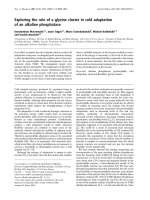
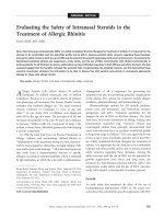
Figure 1 Diagram giving an overview of the admixture process. When two populations admix, genetic recombination starts breaking
ancestral genomes into blocks of different sizes, so that the genomes of the descendants of an admixture event are composed of different
combinations of these ancestral blocks. The number and width of the admixture blocks contain information about the time since admixture, as
more recombination events result in a greater number of blocks, which with time get progressively narrower and more evenly spread along and
among chromosomes.
Pugach et al. Genome Biology 2011, 12:R19
/>Page 2 of 18
overview of the method; the actual methodology is for-
mally developed in the MaterialsandMethodssection
below.
We start by performing a sequential stepwise PCA
(StepPCO) along each chromosome of an individual
from an admixed population and of individuals from
respective parental populations. We consider an
admixed population as a mixture of two ance stral popu-
lations, in which the admixture occurred at a single
timepoint, and assume that no genetic drift occurred
after the admixture event. These, of course, are simplify-
ing assumptions, as most human populations are
expected not only to have many incidents of admixture

occurring at different points in time, and between differ-
ent populations, but also to experience genetic drift rela-
tive to the parental populations. We try to circumvent
this i ssue by finding the first principal axis (PA1) based
on the samples from the proposed ancestral populations
or their proxies, and t hen project the admixed dataset
onto the axis of variation defined by these ancestral
populations, thereby excluding any signal which poten-
tially could originate from drift and/or other sources of
ancestry [8,20]. We t hen consider a sliding window
along each chromosome. The size of this window is not
fixed, but at eac h position is determined by the statisti-
cal properties of the collection of SNPs in the window.
We take evenly spaced points along each chromosome
(evenly spaced in terms of genetic distances); and each
point serves as center for the next window. The number
of points (windows) is chosen so that the windows span
the entire chromosome, leaving no gaps in between. To
simplify subsequent wavelet transform analysis, we also
want the number of windows (or bins) equal to a power
of two. Starting from the center of each window, we
increase the window unt il the mean PC1 coordinates for
the parental populations are separated by three standard
deviations from each mean. The goal is to achieve a
complete separation of the parental populations within
each window, so there is no ambiguity in assigning
chromosomal segments in an admixed genome to either
ancestral population. Because human populations are
closely related, there is an obvious trade-off between the
signal resolution and uncertainty in ancestry estimat ion;

by making the size of the window v ariable and depen-
dent on the number of informative sites within a given
chromosomal region, we always find the smallest possi-
ble window that gi ves us optimal signal resolution with-
out introducing excess errors into the ancestry
estimation. Using PA1 coefficients as weights, we find
the average value of SNPs within each window. The
resulting values are then normalized, so that the ances-
tralpopulationscorrespondtovalueswithmeansof1
and -1, respectively. Thus, for each individual we obtain
a value for each of the windows, and the windows are
evenly spaced along the chromosome. For an admixed
individual, the value in each window will either corre-
spond to one of the ancestral populations, or have an
intermediate value corresponding to having one chro-
mosomal segment from each ancestral population (we
use unphased data , as phasing at the level of an entire
chromosome infers haplotypes with significant phasing
(switch) errors [14,21], making such data unusable for
time since admixture estimation). Thus for each indivi-
dual and each chromosome we obtain a StepPCO signal,
consisting of a sequence of values along the given chro-
mosome. This part of the method is similar to a recently
published approach [10], in which local genomic admix-
ture estimates are inferred using PC analysis on a grid
of points along the genome (and not genome-wide);
unlike our method this approach works with very small
windowsof15SNPs,andrequiresaHiddenMarkov
Model (HMM) to infer ancestry state within each win-
dow. Our implementation is also different in that we

not only estimate the local genomic level of admixture,
but also use the identified ancestry block structure to
date admixture events.
As mentioned earlier, because most SNPs are not
fixed betwee n human populatio ns, it is necessary to use
relatively large windows in order to have enough power
to reliably assign chromosomal segments to an ancestral
population. Large windows mean that the exact location
and width of ancestral blocks in empirical data is diffi-
cult to determine, because small but informative blocks
may be missed, while larger blocks that are actually
noise may be inflated and falsely considered a true sig-
nal. Therefore rather than to attempt a direct estimation
of the number of breakpoints [17] we have developed a
method based on spectral analysis o f the signal using
Haar wavelets [22]. T he wavelet transform represents
the StepPCO signal (described above), as the sum of
simple waves, each characterized by frequency (or per-
iod), and position. These wave frequencies are then used
as a measure of th e width of the ancestral blocks. There
are several advantages to the wavelet transform
approach. First, wavelet transform of the discrete signal
is lossless, and describes the data completely [22]. That
is, wavelet transform coeffiicients could be used to
recover the original signal exactly. Second, wavelet
transform also allows for the reduction of noise, which
in this context is defined as high frequency or low
amplitude oscillations that are not informative but may
falselybeconsideredastruesignals.Byremovingfrom
the analysis wavelet coefficients corresponding to the

high frequency or low amplitude waves within the sig-
nal, we are able to greatly reduce the noise and distill
the a dmixture signal contained within the data. Finally,
the dominant frequency present in the signal is related
to the average width of t he admixture b locks, and can
Pugach et al. Genome Biology 2011, 12:R19
/>Page 3 of 18
thereforebeusedtoinferthetimeofadmixture(see
Materials and Methods, Wavelet Transform section for
details).
Since the recombination rate is uneven along the
chromosome, with 80% of recombination events in
humans occurring w ithin hotspots [23], to measure dis-
tances along the chromosome we use genetic map dis-
tances (measured in cM) rather than physical distances
(measured in base pairs). We interpolate genetic dis-
tances from genome-wide recombination rates estimated
as part of the HapMap project [24].
Simulations
Initial validation of the method was done using an in-
house forward simulation approach. We start with two
distinct populations (A and B), simulating chromosomes
as an interval from zero to one. We choose the recom-
bination rate to be 2.78 events per chromosome per
generation, which corresponds to the recombination
rate observed for human chromosome 1 [25,26]. At
time T
0
the effective population size of population A
equals 1,000 individuals, and it receives either 1%, 5%,

10%, 20%, 30% or 40% migrants from population B. The
simulation then runs forward for 2,000 generations; the
population at each generation is split randomly into
pairs and each pair produces a random n umber of off
spring, drawn from the Poisson distribution, with the
average depending on the specified growth rate. The
growth rate is chosen so that the population grows from
an effective size of 1,000 to 10,000 in 2,000 generations.
Since we are only interested in the dynamics of recom-
bination, we only keep track of the recombination
points, with their coordinates along the chromosome
given a s percentages of the total length of the c hromo-
some. This significantly reduces computational time and
makes modeling of the recombination dynamics feas ible.
We ran indepe ndent sets of simulations using either the
genetic map [25], or the physical position map with
variable rates of r ecombination along the chromosome,
using previously-described parameter values for the
strength and s pacing of hotspots [ 27]. The recombina-
tion map was generated at the beginning of each simula-
tion run. We ran 100 simulations for each of the
migration parameters, and from each simulation we
sampled 100 chromosomes at expon entially growing
time points, and collected statistics on the total amount
of admixtur e, the nu mber of breakpoints, and the width
of admixture blocks (as measured by the wavelet trans-
form coefficients) for each chromosome in each sampled
generation.
The overall admixture rate estimates we obtain are
highly concordant with the migration rate parameter

initially set for each simulation, and this estimation is
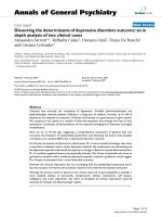
not influenced by the time since admixture (Figure 2a).
Thenumberofbreakpointsvs.time(Figure2b)is
almost linear, with little oscillation within each s imula-
tion. There seems to be a stochastic period immediately
following the admixture event, when random processes
appear to strongly influencetheslope.Ingeneral,the
number o f breakpoints grows faster with higher admix-
ture rates (Figure 2b). Up to about 50 generations, the
number of observed breakpoints closely matches the
expected value:
NTREE
bkpts gen
((1 )var ),= 2
 
−−
(1)
where N stands for the number of breakp oints, T
gen
denotes time since admixture in generations, R corre-
sponds to the number of recombination events per gen-
eration, a denotes the admixture rate for an individual,
and Ea and var a are the mean and the variance of a.
The deviation of the observed number of breakpoints
from that expected after 50 generations (Figure 2b) is
due to the fact that infinite populations the pattern of
ancestral blocks (their width and distribution along
chromosomes) becomes more uniform with tim e, that is
the recombination events are no longer independent.
For the calculation of the wavelet transform (WT)

coefficients, simulated chromosomes we re randomly
paired to form diploids to match the empirical data.
Also, from the calculated WT coefficients we exclude all
coefficients describing high frequency wavelets (WT
levels higher than level seven, as described in the Mate-
rials and methods, Wavelet transform section) and nor-
malize for the length of the chromosome by subtrac ting
the log of the chromosome length, which would corre-
spond to the threshold and normalization imposed on
the e mpirical data for chromosome 1 (as the simulated
chromosomes were of the same length as chromosome
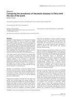
1). The distributions of the WT levels, indicating how
the wavelet transform spectrum changes with time since
admixture, are presented in Figure 3. With time t he
center of the WT spectrum shifts from left to right,
from predominantly low to predominantly high fre-
quency wavelets. In Figure 2c the WT centers calculated
for different time points are plotted against time since
admixture. The centers increase exponentially with time,
are fairly independent of admixture rate, and a re very
consisten t across simulations, especially if the admixture
rate is over 1%. This measure starts to level off at
approximately 400 generations since admixture, which is
due to the elimination of levels containing wavelets of
highest frequency (done to concur to the filtering
applied to the empirical data). For the empirical data,
this removal of high-frequency wavelets is done to
remove noise, which in turn reflects the relatively low
density of informative SNPs present in the data; with
more dense SNP data (or full sequence data), we would

Pugach et al. Genome Biology 2011, 12:R19
/>Page 4 of 18
expect to have more power to detect more ancient
admixture events.
Sensitivity of the method to smaller effective population
size and continuous migration
To test the sensitivity of our method with respect to the
initial effective population size, we ran additional simula-
tions where the effective size of population A at T
0
equals
500 or 200 individuals, and it receives either 5%, 10% or
20% migrants from population B. The growth rate of the
new admixed population was chosen so that in 2,000 gen-
erations the population grows to 10,000 or 2,000 indivi-
duals, respectiv ely. Results are shown in Figure S1 in
Additional file 1. There is no influence of initial population
size on the performance of the method for admixture
times up to about 20 generations ago. For populations
with small Ne and admixture events older than 20 genera-
tions ago, our approach will tend to overestimate the date
of admixture for more recent events, and not be able to
detect more ancient events. Apparently, the diversity in
the distribution of ancestry blocks diminishes (stabilizes)
faster in smaller populations, thus making new recombina-
tion events undetectable. The same phenomenon is
responsible for the deviation of the number of recombina-
tion breakpoints observed in our simulations from the
value predicted by Equation 1. Our results further suggest
that it is not so much the small Ne, but rather the growth

rate of the population, which is primarily responsible for
these deviations. Moreover, the effect is more pronounced
when the admixture rate is low.
Additionally, we ran simulations to test how continu-
ous admixture over time affects the method. Again we
start with a population A, which at T
0
comprises 1,000
individuals, and it receives either 5% or 20% migran ts
from population B over the period of either 10 or 30
generations. The growth rate of the new admixed popu-
lation was chosen so that in 2,000 generations the popu-
lation grows to 10,000, and 100 simulations were
performed for each scenario. Results are shown in
Figure S2 in Additional file 1. Because new ancestry
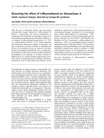
Figure 2 Data from 100 simulations for m igration values of 1%, 5%, 10%, 20%, 30%, and 40%. Each curve represents a single admixed
population. To generate the plots, 100 chromosomes were sampled from each population at exponentially growing time points, and the
following statistics for each chromosome in each sampled generation were collected: (a) admixture rate; (b) number of breakpoints; black lines
indicate the expected value, given by: N
bkpts
=2T
gen
R(Ea(1 - Ea) - var a); and (c) the WT centers. Inset: Average number of breakpoints for each
simulation parameter. Black lines indicate the expected value.
Pugach et al. Genome Biology 2011, 12:R19
/>Page 5 of 18
blocks are being continuously introduced over the per-
iod of either 10 or 30 generations, potentially removing
older block structure by replacing narrower ancestry
blocks with new wider blocks, we expect ongoing

admixture to reduce the wavelet transform coefficients
and therefore lead to an underestimation of t ime since
admixture. This is indeed what we observe: irrespective
of the admixture rate throughout the duration of admix-
ture (10 or 30 generations), the wavelet transform coeffi-
cients are lower than those observed in a population
with the same admixture rate, but which has experi-
enced not a continuous but a one-time admixture event.
Once the influx of new genetic material into the simu-
lated populatio n A stops, the trajectory of growth of the
wavelet transform coefficients is slowly recovered.
Sensitivity of the method to levels of linkage
disequilibrium
As describe d in the Overview of the Method, to measure
distances along the chromosome we use ge netic map
distances (measured in cM) rather than physical distances
(measured in bp). As we meas ure distances in units of
recombination frequency, chromosomal regions with high
LD, that is low propensity towards recombination, will
span smaller distances and be represented by a smaller
number of windows, and conversely genomic regions that
harbor recombination hotspots will be inflated and repre-
sented by a larger number of windows. We therefore do
not expect levels of LD to affect our results. To demon-
strate this we have measured LD [28] in fixed windows
across chromosomes 6 and 8 in three HAPMAP popula-
tions: indivi dua ls of E uropean ancestry (CEU), the Yoruban
(YRI) individuals and the indivi duals of African ancestry
from the Southwestern USA (ASW). Genotype data were
downloaded from the International HapMap project home

page [29]. The size of the fixed window was chos en as a
fraction of a chromosome length to correspond on average
to either 500 kb or to 0.5 cM. In accordance with our
expectations we observed that the level of LD varies along
the chromosome if the distances are measured in base
12345678910
0.00 0.04 0.08 0.12
2.95
Levels
12345678910
0.00 0.04 0.08 0.12
3.95
Admixture 12 generations ago
Levels
12345678910
0.00 0.04 0.08 0.12
4.95
12345678910
0.00 0.04 0.08 0.12
5.57
12345678910
0.00 0.04 0.08 0.12
6.07
Admixture 90 generations ago
12345678910
0.00 0.04 0.08 0.12
6.85
Admixture 205 generations ago
12345678910
0.00 0.04 0.08 0.12

7.35
Admixture 438 generations ago
12345678910
0.00 0.04 0.08 0.12
7.65
Admixture 2000 generations ag
o
Admixture 3 generations ago
Admixture 32 generations ago
Admixture 57 generations ago
Levels Levels
L
e
v
e
l
s
L
e
v
e
l
s
L
e
v
e
l
s
L

e
v
e
l
s
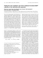
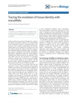
Figure 3 Distributions of the WT levels, illustrating how the wavelet transform spectrum changes with time since admixture. For each
illustrated time point, WT levels from 10 randomly chosen simulations are plotted (each bar represents one simulation, resulting in 10 bars for
each level). The height of the columns indicate the abundance of wavelets of particular frequency present in the signal, starting with the lowest
wave frequencies (widest recombination blocks) on the left and progressing towards the highest wave frequencies (narrowest recombination
blocks) on the right. The WT centers in this plot are not adjusted for chromosome length, and thus appear to be higher than the values we
present for genomewide data.
Pugach et al. Genome Biology 2011, 12:R19
/>Page 6 of 18
pairs, but does not vary as much if the distances are mea-
sured in cM (Figure S3 in Additional file 1).
Sample size estimation
For some of the populations considered in this study the
sample size was limited to 25 individuals. To ensure that
the S tepPCO method has adequate power, we therefore
calculated how large a sample size is required for accu-
rate and reliable estimates of admixture time. We
sampled from 1 to 50 individuals at random from one
randomly-chosen simulated population at 12 different
time points. Average WT centers, based on different
sample sizes, were calculated and used to infer time
since admixture by comparing the observed WT cent ers
to those obtained using the entire simulated dataset.
The results (Figure S4 in Additional file 1) indicate that
asamplesizeof10issufficientforquiteaccuratetime
estimation with narrow confidence intervals up to about

200 generations ago. Point estimates become less pre-
cise, and confidence intervals become much wider, at
time points exceeding 500 generations ago. This is
caused by the threshold imposed on the simulated data
to concur with the same limitation that is present in the
empirical data, due to the elimination of levels contain-
ing wavelets of highest frequency (removal of noise, as
described above).
Comparison to HAPMIX: simulated data
Various methods have been developed to quantify the
admixtu re signal along indiv idual chromosomes, such as
ANCESTRYMAP [4], SABER [14], LAMP and LAMP-
ANC [15], uSWITCH and uSWITCH-ANC [16], and
HAPMIX [17]. To test the performance of the StepPCO
approach relative to these other programs, we chose to
compare the method only to HAPMIX, as this approach
has been shown to perform better relative to the other
methods in predicting ancestry transitions, especially for
smaller ancestry segments which carry information on
more ancient admixture events [17].
To compare to HAPMIX, we constructed an artificially
admixed dataset from the phase d genotypes of the Yoru-
ban (YRI) individuals and individuals of European ances-
try (CEU), downloaded from the International HapMap
project home page [30]. Forty haploid admixed genomes
were constructed as described previously [17], namely for
each simulated chromosome we randomly selected one
haploid Yoruban and one haploid CEU genome, and
built a recombination map by drawing from an exponen-
tial distribution with weight l, such that the ancestry

switch occurred with probability 1 - e
-lg
for each distance
of g Morgans. Starting a t the beginning of each chromo-
some and at each of the recombination points from the
recombination map, we sampled European ancestry wit h
probability a and African ancestry with probability 1 - a,
where the value of a was sampled once from a beta dis-
tribution with mean 0.20 and standard deviation 0.10,
typical for African Americans [17]. We simulated the fol-
lowing values of l: 6, 10, 20, 40, 60, 10 0, 200, 400. Once
an artificial genome was constructed, parental chromo-
somes were never reused. Pairs of the resulting artific ially
admixed haploid geno mes were merged to create 20
diploid admixed individuals.
We then compared the performance of our spectral
decomposition method to HAPMIX on these artificially
admixed genomes. We ran a StepPCO analysis, followed
by the W T decomposition of the resulting StepPCO
admixture signal. To investigate how the dominant wave-
let frequency is rel ated to l for this a rtificial dataset, we
generated a separate dataset of hybrids. Maps of recombi-
nation events for each of these additional hybrid genomes
for the values of l: 6, 10, 20, 40, 60, 100, 200, 400 were
constructed as described in the previous paragraph. 20
hybrids genomes were constructed for each value of l,
and spectral decomposition analysis was carried out on
the resulting admixtur e signal. Using the known number
of breakpoints in these simulated hybrids, we have found
that the dominant wavelet frequency is linearly related to

the logarithm of the average (per Morgan) number of
ancestry switches (breakpoints); linear regression was
used to find the coefficients, and estimate the average
number of ancestry switches per unit of genetic distance
in the main simulated dataset.
We also ran HAPMIX on the same artificially-
admixed samples, using 40 haploid YRI and 40 haploid
CEU genomes as the reference parental populations and
using the input parameters recommended previously
[17]. We calculated the number of ancestry switches
detected by HAPMIX, as the output of HAPMIX pro-
duces probability associated with each SNP genotype in
the admixed g enome. We then compared the true num-
ber of ancestry switches per Morgan of genetic distance
(known for simulated data) to the estimates produced
by either HAPMIX or WT decomposition of the admix-
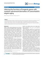
ture signal. The results (Figure 4) show that HAPMIX
consistently underestimates the number of breakpoints,
while the estimates obtained by the WT analysis are
more accurate, especially for higher values of l, typical
of more ancient admixture events.
However, accurate estimation of breakpoints does not
imply accurate estimation of the admixture time. As
demonstrated previously (Figure 2b), the number of
breakpoints can deviate significantly from the value pre-
dicted by Equation 1, especially with higher admixture
rates, lower ancestral Ne, and/or older admixture times.
Furthermore, inference of breakpoints requires transfor-
mation of the ‘raw’ genomic signal into a discrete signal
corresponding to the presence or abse nce of an ancestry

switch, hence direct inference of number of b reakpoints
Pugach et al. Genome Biology 2011, 12:R19
/>Page 7 of 18
is inevitably error-prone. These errors, however small,
will accumulate over the many measurements taken.
WT analysis avoids such errors because rather than
inferring the recombination events directly, the WT
method compares the spectral properties of the given
signal in the observed data with the properties of the
model signal produced by simulations.
Empirical data
Quality-filtered genotypes for approximately one million
SNPs for 25 Polynesians (PLY), 25 Fijians (FIJ), 23
Borneans (BOR) and 25 individuals from the highlands
of Papua New Guine a (MEL), typed with Affymetrix 6.0
arrays, were obtained from a previous study [19] and are
available from the authors upon request. Quality-filtered
genotypes obtained with the Illumina Human1 M and
Affymetrix 6.0 arrays for 20 Yorubans from Ibadan,
Nigeria (YRI), 20 individ uals of nor thern and western
European ancestry living in Utah (CEU) and 20 indivi-
duals of African ancestry from the Southwestern USA
(ASW), were downloaded from the Internatio nal Hap-
Map project home page [29]. SNPs were merged using
True number of break
p
oints
p
er cM
Predicted number of breakpoints per cM

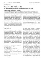
Figure 4 Performance of Hapmix and wavelet transform analysis in recovering the average number of recombination breakpoints per
Morgan of genetic distance from simulated data. The two methods were applied to 20 artificially admixed individuals, created using a
genomewide average of 20% European and 80% African ancestry. For simulated data the average number of ancestry switches (or breakpoints)
was drawn from an exponential distribution with weight l, such that the ancestry switch occurred with the probability 1 - e
-lg
for each distance
of g Morgans. The following values of l were simulated: 6, 10, 20, 40, 60, 100, 200, 400. Since in the simulated genomes the true number of
breakpoints is known, we show the accuracy of both methods in recovering this information.
Pugach et al. Genome Biology 2011, 12:R19
/>Page 8 of 18
the PLINK tool [31], to include only markers which
were genotyped and passed the quality filters in both
datasets. The final dataset comprised 653,498 SNPs. We
also analyzed and dated admixture in Mandenka, Moza-
bite, Bedouin, Palestinian and Druze groups from the
CEPH-HGDP [18]. These groups were previo usly ana-
lyzed via HAPMIX and reported to have European-
related ancestry ranging from 2% to 97%, when analyzed
using Africans and Europeans from the HapMap as the
input reference populations [17]. These samples were
genotyped for 650,000 SNPs on the Illumina platform
[18]. The data were downlo aded from the HGDP CEPH
Genotype Database [32].
For the empirical admixture analyses, the parental
groups are: the French and Yoruba for the admixed
Mandenka, Mozabite, Bedouin, Palestinian and Druze
groups; the YRI and CEU groups for the admixed ASW
group; the BOR and MEL groups for the admixed PLY
group; and the MEL and PLY groups for the admixed
FIJ group. The StepPCO approach was first used to elu-

cidate the local structure of the admixture signal for
each admixed individual along each chromosome. We
then estimated admixture proportions in each admixed
group, and compared the StepPCO results for each
chromosome to admixture proportions estimated using
the maximum-likelihood based algorithm implemented
in frappe [13]. We then applied wavelet transform analy-
sis to the StepPCO signal and used the wavelet trans-
form coefficients to infer time since admixture. After
the wavelet transform coefficients were calculated we
applied t hree filtering procedures to the signal. First, as
explained previously, we replaced all coefficients smaller
than an ascertained threshold value by zero, to remove
low amplitude oscillations that are characteristic of
noise (that is, wavelets of low height). This threshold
value was chosen so that small oscillations present only
within the distribution of the parental individuals are
ignored. Second, we removed WT levels that correspond
to the wavelets of the highest frequencies, which are
also characteristic of noise (that is wavel ets that are too
narrow). Then we averaged the coefficients a cross each
level and found a thresho ld ampli tude, which is present
in every individual whether admixed or not, and con-
sider everything below it as noise (in effect this means
that we subtract the parental signal, that is when we
analyze the admixture signal in FIJ for example, with
PLY a nd MEL being the ancest ral populations, the fact
that PLY themselves harbor Melanesian admixture has
no effect on the inference of the admixture date for FIJ).
Finally, we find the dominant frequency present in the

signal (WT center) and use it to infer the time of
admixture by comparing this observed dominant fre-
quency to that obtained in simulated data generated
using the admixture rate observed in the empirical data.
African-Americans, Polynesians and Fijians
StepPCO plots for one ASW, one PLY, and one FIJ are
presented in Figure 5. The pattern of chromosomal seg-
ments alternating between two ancestral states is char-
acteristic of all admixed individuals and is observed on
all chromosomes. For some chromosomal segments
intermediate PCA1 values are observed, indicating that
the admixed individual contai ns chromosom al segments
from both parental populations (see Figure S5 in Addi-
tional file 1 for StepPCO results for the other chromo-
somes from these three individuals). As described in the
Overview of the Method, the number of SNPs per slid-
ing w indow of the StepPCO analysis is allowed to vary,
in order to achieve reliabl e assignment of chromosomal
segments in admix ed individual s to the corre ct parental
group. The average number of SNPs per StepPCO slid-
ing w indow for chromosome 1, which contained a total
of 42,499 SNPs a fter filterin g, was: 280 for African
Americans, 519 for Polynesians, and 1015 for Fiji. This
variation reflects the different levels of differentiation
between the ancestral populations of these three
admixed groups. The largest average size of the sliding
window is observed for Fiji, where PLY and MEL are
used as parental groups. As the PLY themselves have
Melanesian ancestry, PLY an d MEL are much less dif-
ferentiated than CEU and YRI, the parental populations

of the African Americans. Hence more SNPs are needed
to reliably assign chro mosomal segments in the FIJ
group to either of the ancestral populations, than are
needed for the ASW.
Average admixture proportions estimated by the
StepPCO method for the African-Americans, Polyne-
sians and Fijians are 19% European ancestry, 24.9% Mel-
anesian ancestry, and 40.2% Melanesian ancestry
respectively (Figure 6a). Individual admixture estimates
vary substantially a mong the African-Americans, with
some individuals exhibiting very low European ancestry
(less than 5%), and some substantially higher (more
than 40%). These results were substantiated by the
frappe [13] analysis, which agree quite closely with the
per-chromosome ancestry estimates from the StepPCO
analysis (Figure 6b). A similar pattern is observed in Fiji,
with Melanesian ance stry ranging from 22% to 63%.
Despite the fact that the Polynesian sample is very
diverse, coming from seven different islands [19], the
level of Melanesian ancestry is much more uniform
across individuals (varying from 18 to 28%).
The spectral analysis of the StepPCO signal revealed
that the average dominant frequency for the African-
Americans is located at level 1.8, which would corre-
spond t o an abundance of low frequency wavelets (that
is, wider ancestry blocks), while for the Fijians and the
Polynesians the average dominant frequency is at level
3.06 and 3.63 respectively, which is indicative of much
Pugach et al. Genome Biology 2011, 12:R19
/>Page 9 of 18

PC1
PC1PC1
PC1
PC1
PC1
PC2
PC2
PC2
Position (cM) Position (cM) Position (cM)
CEU
YRI
ASW_19819
Borneo
New Guinea
Polynesia_22
New Guinea
Polynesia
Fiji_24
StepPCO: Chromosome 1
(a)
(b)
(c)
Figure 5 PCA and StepPCO results for chromosome 1. Solid lines centered around 1 and -1 indicate the mean PC1 coordinate for each
parental population; progressively lighter shading surrounding the mean of each parental group indicate +/-1, +/-2 or +/-3 standard deviations
from the mean. (a) Upper panel: PC1 vs PC2 for populations of CEU, YRI and ASW. Lower panel: Unphased chromosome 1 of an individual of
African American ancestry; European (blue) and Yoruba (red) populations are used as parental groups. (b) Upper panel: PC1 vs PC2 for
populations of MEL, BOR and PLY. Lower panel: Unphased chromosome 1 of an individual from Polynesia; Borneo (green) and New Guinean
(orange) populations are used as parental groups. (c) Upper panel: PC1 vs PC2 for populations of MEL, PLY and FIJ. Lower panel: Unphased
chromosome 1 of an individual from Fiji; Polynesia (brown) and New Guinean (orange) populations are used as parental groups.
ASW: 19%

FIJ: 40.2%
0.0 0.1 0.2 0.3 0.5 0.6
0.4
ASW
PLY FIJ
PLY: 24.9%
Estimated % admixture
Genome-wide admixture
Frappe and StepPCO results
Chromosome 1:
F: Frappe estimates
S: StepPCO estimates
Estimated admixture
(a)
(b)
Figure 6 Admixture estimates. (a) Genome-wide admixture estimates based on StepPCO for African-Americans, Polynesians and Fijians. (b)
Comparison of admixture estimates obtained via StepPCO vs. Frappe, for chromosome 1 for 20 African-Americans.
Pugach et al. Genome Biology 2011, 12:R19
/>Page 10 of 18
narrower ancestry blocks (Figure 7). Based on simula-
tions, the WT center of 1.8 corresponds to an admixture
time of 6 generations ago (95% CI: 4-8 generations) for
the African Americans. Assuming a generation time of
30 years [33], our results indicate that the admixture in
the African Americans started about 180 years ago.
Similarly, the simulations indicate that the WT center of
3.63 for the Polynesians corresponds to an admixture
time of 90 generations (95% CI: 77-131 generations), or
about 2,700 ye ars ago (Figure 8). The time estimation
for Fiji is based on simulated data with a 40% admixture

rate (to match the higher admixture rate of Fiji), and
here the WT center of 3.06 corresponds to an adm ix-
ture time of 37 generations (95% CI: 29-39) or about
1,100 years ago.
HGDP populations
To test how the performance of our approach compares
to HAPMIX, we applied our method to the Mandenka,
Mozabite,Bedouin,Druzeand Palestinian populations
from the CEPH-HGDP [18], which were previously ana-
lyzed using HAPMIX [17]. The HAPMIX estimates for
the European-related ancestry in these populations ran-
ged from 2% to 97%, when analyzed using Africans and
Europeans from the HapMap as the input reference
populations(Table1).Thetimesinceadmixturein
these populations was inferred by calculating the num-
ber o f genomewide ance stry transitions (or the number
of breakpoints), and the results are reported in Table 1.
Although we estimated simil ar admixture proportions
for these populations (Table 1), subsequent spectral ana-
lysis of the admixture signal in the Mandenka, Mozabite,
Bedouin, Palestinian and Druze revealed older admix-
ture dates for the Mozabites and the Druze populations
(Table 1 and Figure S6 in Additional file 1). The
Bedouin population appears to be structured, with
24 out of 45 individuals having a much higher propor-
tion of European-related ancestry (Figure S7 in Addi-
tional file 1). If these individuals are removed f rom the
analysis, the estimate for the admixture time in the Bed-
ouins changes to 97 generations ago (CI: 83-131).
All programming and data analysis was performed

using R (ver. 2.10.1) [34]. All scripts are freely available
[35].
Conclusions
Using genetic data to infer the time of migratio ns has
always been difficult, and the time estimates obtained
often come within wide confidence intervals, making
these dates unreliable and inferences problematic. Here,
we have introduced an approach that takes advantage of
dense genome-wide SNP data to improve precision and
reduce bias in making inferences about the timing of
human migrations. By using an admixed population one
can capitalize on the property of the genome to recom-
bine each generation, producing chromosomes that are
a mixtu re of the parental genetic material. The structure
of an admixed genome contains temporal information
about an admixture event, as a greater number and nar-
rower width of ancestry blocks indicates more recombi-
nation events, and hence greater time depth.
Simulations indicate that the WT coefficients can be
used to obtain acc urate estimates of the time of admix-
ture from suitable genome-wide SNP data. We therefore
applied the method to three datasets, consisting of
about 650,000 SNPs, to estimate the amount and time
of admixture for three human populations: African-
Americans, Polynesians, and Fijians. In addition, we ana-
lyzed and dated admixture in five HGDP populations of
African and Middle-Eastern origin. At first g lance, it
may appear that the simulated and empirical data differ
in that the simulations used fully-differentiated popula-
tions, which is not the case for the empirical data. How-

ever, as explained in more detail in the Results and
Discussion (Basic Setup section), the number of SNPs is
adjusted in the StepPCO sliding windows until the
ancestral populations can be statistically-differentiated,
just as with the simulated data.
For African-Americans, we estimate an average of 19%
European ancestry, with a wide range of less than 5% to
ASW: 1.83
PLY: 3.63
FIJ: 3.06
012345
0
12
3
4
5
Mean WT Coeff Centers
Mean level of WT coeff
ASW
PLY
FIJ
Figure 7 Average centers of the WT coefficients, calculated for
each individual.
Pugach et al. Genome Biology 2011, 12:R19
/>Page 11 of 18
ASW: 6 gen ago
FIJ: 37 gen ago
PLY: 90 gen ago
Generations
WT coefficients

Figure 8 Admixture time estimates for the African-Amer icans, Polynesians and Fijians. Simulated data from 100 simula tions with a 20%
and 40% migration rate are presented. Each curve represents a single admixed population. Average WT centers calculated for 100 chromosomes
drawn at random from each population at exponentially growing time points are plotted as a function of time. Measurements obtained for the
ASW, PLY and FIJ populations are shown by blue horizontal lines. Red vertical lines indicate the time estimate, and shaded boxes define the
confidence intervals. Time estimate for ASW and PLY are based on simulations with a 20% admixture rate, while the time estimate for FIJ is
based on simulations with a 40% admixture rate.
Table 1 Comparison of results from HAPMIX and StepPCO
Population Estimated percent
European ancestry from
HAPMIX
Estimated percent
European ancestry from
StepPCO
Estimated time since admixture
(in gens ago) from HAPMIX
Estimated time since admixture
(in gens ago) from StepPCO
Mandenka 2% 2% 120 121
Mozabite 77% 84% 100 131
Bedouin 91% 91% 90 83
Palestinian 93% 92% 75 72
Druze 97% 96% 60 90
We have removed one outlier individual from the Mandenka population. Among the Bedouins, 24 out of 45 individuals have a higher proportion of European-
related ancestry (Figure S7 in Additional file 1). If these individuals are removed from the analysis, the estimate for the admixture time in the Bedouins changes
to 97 generations ago. Estimated percent European ancestry was calculated by using the two parental populations and an admixed group to find the PC1 axis.
Pugach et al. Genome Biology 2011, 12:R19
/>Page 12 of 18
more than 40% European ancestry across individuals.
Both the average and th e observation of a wide range of
individual admixture estimates are in keeping with pre-

vious studies [10,17,36,37]. The estimated time of
admixture is about 180 years ago (95% CI: 120-240
years ago), which is probably an underestimate since
admixture in the African-American population is
ongoing (implying that new ancestry blocks a re being
continuously introduced by new recombination events,
which potentially removes older block structure by
replacing narrower ancestry blocks with new, wider
blocks).
We tested the performance of the method on Fijians
and Polynesians, as both populations are of admixed
Asian and Melanesia n ancestry [6]. Previous demo-
graphic analyses of the genome-wide SNP data used in
this study strongly support both an admixed Asian/Mel-
anesian ancestry for Fijians and Polynesians as well as
subsequent additional gene flow from Melanesia into
Fiji, but not Polynesia [19]. Based on this previously
established scenario, we estimated an average of about
25% (from 18 to 28%) Melanesian ancestry in Polyne-
sians, in good agreemen t with previous estimates based
on the same [19] or other [6,38-40 ] data. The estimated
time of admixture is about 90 generations ago, or 2,700
years (95% CI: 2,300-3,900 years), in good agreement
with a previous est imat e of about 3,000 years ago based
on an ABC simulation approach for the same data [19].
For Fiji, the estimated amount of Melanesian ancestry
was about 40%, and the time for this admixture is esti-
mated to have occurred about 37 generations ago, or
1,100 years (95% CI: 870-1170 years). An ABC-simula-
tion based approach for the same data gave an estimated

date of 62 generations for this admixture in Fijians,
about twice as long ago as our estimate. We speculate
that, as in the case of the African-Americ ans, the esti-
mate based on WT coefficients may be biased toward
more recent dates if the gene flow to Fiji occurred over
a period of time, as more recent gene flow replaces
older, narrower ancestry blocks w ith newer, wider
ancestry blocks. Individual Melanesian ancestry esti-
mates are much wider for Fiji (from 22 to 63%) than for
Polynesia (from 18 to 28%), which may indeed indicate
a longer period of gene flow into Fiji.
OurresultsfortheMozabite,Mandenka,Bedouin,
Druze and Palestinian populations are similar to those
for HAPMIX for inferring local ancestry, and in addition
our method seems to perform better with respect to
more ancient admixture events (as also shown with
simulated data: Figure 4). In particular, we dated t he
admixture event in the Mozabites and the Druze to 1 31
and 90 generations ago respe ctively, 30 generations
more than the corr esponding estimates obtained wit h
HAPMIX [17]. HAPMIX estimation of the time since
admixture is based on the number of calculated ancestry
transitions (that is, the number of breakpoints); both our
simulations and previous simulations [17] indicate that
infinite size populations the number of breakpoints does
not increase with time according to expectations (see
Equation 1 above), but rather stabilizes, leading to
underestim ates in admixture dates (Figure 2b). Furth er-
more, because human populations are closely related
and not very well differentiated, direct estimation of the

number of breakpoints and block width as a measure of
time since admixture for human genetic data is proble-
matic for two reasons. Firstly, to have enough power to
reliably assign chromosomal segments to an ancestral
population, it is necessary to use relatively large geno-
mic w indows, which correspondingly reduces detection
of closely-spaced breakpoints. And secondly, for every
location in the genome that potentially carries a break-
point, a formal decision has to b e made as to whether
to consider i t a true breakpoint or not. This transforma-
tion of the ‘raw’ signal into a discrete signal potentially
leads to either some not well-defined breakpoints being
overlooked, or converse ly random effects becoming
inflated and falsely considered as a true signal. These
errors, however small, will accumulate over the many
measurements taken. Conversely, the spectral analysis
approach implemented here does not require any data
transformation and is applied to the ‘raw’ signal directly.
This has the advantage of p reserving the statistical nat-
ure of the signal until the final averaging step, and thus
does not involve detection of exact location (and pre-
sence) of breakpoints, w here inevitably large errors in
estimation could occur. Although we followed Price et
al. 2009 in using African and European parental groups
for the admixed Mozabite, Mandenka, Bedouin, Druze
and Palestinian groups from the CEPH-HGDP, in fact
previous studies have shown that the Druze, Bedouin
and Palestinian populations are admixed primarily along
a European-Central Asian axis, with little African
admixture, and the Mandenka exhibit very little Eur-

opean admixture [18,41]. Here, we report dates for the
presumptive European gene flow, to compare our results
to the previous study [17], but it is important to keep in
mind that our method (like all admixture methods)
requires the u se of pre-defined parental groups. Incor-
rect identification of the ancestral groups contributing
to an admixed group will obviously lead to erroneous
conclusions, hence careful attent ion must be paid when
identifying parental groups. This is especially true fo r
groups that are suggested to have experienced admix-
ture a l ong time ago, and hence had more time to
experience genetic drift (which is always expected to act
in a direction orthogonal to the axis of admixture). In
such cases, it is difficult to distinguish between an
admixed population that has been subject to gen etic
Pugach et al. Genome Biology 2011, 12:R19
/>Page 13 of 18
drift, and a population that has experienced admixture
along a different axis of variation.
Theoretically, there are no limitations as to how far back
in time one can get good estimates of admixture time with
WT coefficients. The performance of the method is influ-
enced by two factors: the density of SNPs analyzed and
the degree of differentiation between the two parental
populations. Increasing SNP density would allow the esti-
mated time horizon for detecting admixture to be moved
further back. We therefore expect that full sequence data
will increase the sensitivity and resolution of our method.
The analysis presented here was based on ab out 650,000
markers; the current estimates for the number of SNPs in

the human genome is around 15 million SNPs [42]. Full
sequence data will thus provide a twentyfold increase in
SNP density, and thereby allow for a twentyfold reduction
in the size of the sliding window. Thus, assuming that the
newly added SNPs are no less informative for populatio n
differentiation than the SNPs on the Affymetrix arrays, we
expect that analysis of full sequence data should offer at
least a twentyfold improvement in the potential time
depth for admixture estimates for human populations.
However, given that there is relatively little genetic differ-
entiation between human populatio ns, to disting uish
among parental populati ons requires relatively large seg-
ments of the genome, and this also poses a restriction on
the time depth of the method. The more closely-related
the parental populations, the larger the window size
needed to span a sufficient number of informative SNPs.
Obviously, this limitation will persist regardless of the type
of molecular data considered. However, because of the
strong ascertainment bias associated with the SNPs geno-
typed on the arrays, we expect that SNP-data generated
using the array technology necessarily underestimates the
variation that exists between human populations, and
recent studies suggest that this underestimation could be
considerable [43]. Moreover, the method introduced here
can be used with any species for which suitable genome-
wide data exist, and the larger the genetic difference
among the parental populations, the less genome-wide
data needed for accurate admixture estimates.
An additional advantage of the StepPCO method is that
it provides an estimate of the admixture proportions for

each individual within an admixed population. Individual-
level estimates of admixture obtained here via StepPCO
for African-Americans, Polynesians, and Fijians were quite
similar to those obtained via the maximum-likelihood
based approach frappe [13], indicating that StepPCO gives
reliable results. Furthermore, the StepPCO method also
provides information about the distribution of admixture
along each chromosome. As such, this approach is also
promising for disease gene mapping (in recently admixed
populations), and for studying local selection. According
to neutral expectations the admixture level should be
constant along the genome, but a locus favored by positive
selection in the admixed population should appear to have
greater admixture proportions than would be expected
from the genome-wide average. We are currently investi-
gating the utility of this approach for identifying candidate
genes subject to local selection.
In conclusion, we have shown that wavelet transfor-
mation is a useful and novel means of dating admixture
events from genome-wide data. Other potential exten-
sions of the methodology i ntroduced here include
admixture scenarios involving more than two parental
populations, and implementing spectral analysis of the
raw genomic signal directly, rather than from the
StepPCO signal. There is potentially much more to be
learned from surfing the wavelets of the genome.
Materials and methods
Basic setup
We consider a collection of N SNPs along a chromo-
some, which are ordered by their physical position, and

indexed by numbers from 1 to N. For such a collection
of SNPs we consid er a vector
p :( )=
=
p
ii
N
1
of each SNP’s
physical position along the chromosome scaled with
respect to the genetic distances, which were interpolated
from genome-wide recombination rates, estimated as
part of the HapMap project [24]. Suppose e is an indivi-
dual chromosome. We also denote
e :()=
=
e
ii
N
1
as a col-
lection of calls at given SNP positions for the
chromosome e. E ach component in the vector e for
each individua l chro mosome takes value 0, 1, -1 or NA,
where - 1 and 1 are assigned to the two possible homo-
zygotes of a given SNP and 0 corresponds to a heterozy-
gote. The space of all possible calls (excluding NAs) sits
as a discrete set in an N-dimensional real vector-space E
with canonical basis.
We then consider a sliding window along each chro-

mosome. Such window w refers to a contiguous sub-
range of SNPs, that is:
w =+−
{}
ww w w
first first last last
, , , , .11
The width of a window is defined by the genetic dis-
tance between the last and the first SNP in the window:
Width
last first
w
()
=−:.pp
ww
Suppose we are given an oriented line A in the vector-
space E (later A will be taken to be a principal axis of a
certain collection of individual chromosomes). Line A is
spanned by a single non-zero vector with coordinates
a
i
i
N
()
=1
defined up to mult iplication by a positive
number.
Pugach et al. Genome Biology 2011, 12:R19
/>Page 14 of 18
For a given window w and an individual chromoso me

e, define a measurement associated with this window
with respect to the axis A by:
M
ae
a
ii
i
i
i
w
w
w
e():
||
.=
∈
∈
∑
∑
Obviou sly, the resulting value does not depend on the
choice of a vector spanning A.
Given a point x along the chromosome, we say that a
window w is centered at a point x and has a width l if it
consists of exactly those SNPs that lie within the dis-
tance l/2 from x, that is:
w
lw
xwxp
l
(): | | .=−≤

⎧
⎨
⎪
⎩
⎪
⎫
⎬
⎪
⎭
⎪
2
Consider sample collections {p
k
}and{q
k
}fromtwopopu-
lations P and Q, respectively. Let
a =
=
()a
ii
N
1
define the
principal axis in SNP-coordinates for a collection of sam-
ples {p
k
,q
k
}. Given a point x

0
along the chromosome and a
window w centered at this point, consider measurements:

kk kk
Mp Mq:() :().==
ww
and
Given a positive real number l > 0, we say that popu-
lations P and Q are l-separated in a window w if:
|||()()|,EE

−≥ +
(2)
where E stands for the mean and s for the standard
deviation estimators of the PC1 coordinate of popula-
tions P and Q.
Finally, a window w is called l-optimal if it has the smal-
lest size, such that populations P and Q are l-separated in
w (that is the smallest possible window that satisfies Con-
dition 2). The size of this window at each position is cho-
sen so that the ancestral populations are sufficiently well
separated by the statistica l properties of the collection of
SNPs in the window. We set l =3,thatisweconsidera
window as optimal, when the mean PC1 coordinates for
the parental populations are separated by three standard
deviations from each mean. Note that in general the opti-
mal size will depend on the position of the window along
the chromosome. In effect, by taking smaller windows in
chromosomal regions that contain more informative

SNPs, we are able to increase signal resolution without
introducing excess errors into the ancestry estimation.
In summary, for t he sample collections {p
j
} ⊂ P and
{q
j
} ⊂ Q we construct the following data: a) the princi-
pal axis A spanned by a non-zero vector with coordi-
nates
a
i
i
N
()
=1
for a collection of samples {p
j
, q
j
}; b) a
collection of K equispaced points
{}x
kk
K
=1
along the
chromosome; and c) for each point x
k
, k = 1, , K we

construct a l-optimal window w
k
centered at x
k
.These
data we refer to as a StepPCO frame. (Special care
needs to be taken so that the windows cover the entire
chromosome, leaving no gaps in between. This can
always be achieved by choosing the number of bins K
sufficiently large.)
StepPCO
Using coef fici ents of PA1 as weights, we find the average
value of SNPs within a window. The resulting values are
then normalized, so that the ancestral populations corre-
spond to values with means of 1 and -1, respectively.
Consider collections {p
j
}and{q
j
} of samples from
two ancestral populations P and Q and a set of admixed
individuals R ={r
j
}. Construct a StepPCO frame (in our
applications l = 3 and number of bins is K = 1,024).
For an individual chromosome r from population R,
define the StepPCO signal as a vector of measurements:
S(): ( ()) .rr
w
=

=
M
k
k
K
1
Each component of the vector
S()r
characterizes a
stretch of chromosome r corresponding to each bin as
belonging to one of the ancestral populations, and the
confidence of such an assignment. The level of confi-
dence will of course depend on l.
Suppose the principal axis is directed from P to Q.
Then the closer the value of the signal to 1, the more
likely that the corresponding stretch of the chromosome
of the sample r belongs to ancestral population Q.
Analogously, values close to -1 correspond to the
stretches of DNA most likely tracing their ancestry to
population P.
Wavelet transform
Consider a 2
L
-dimensional vector-space
V
L
= 
2
with
the scalar product:

uv uv
ii ii
i
L
()()
=
=
∑
,: .
1
2
Wavelets (ω
l, p
)aretheorthogonalsystemof2
L
-1
vectors in V .Theyareindexedbythelevell = 1, , L
and the position p = 1, , 2
l-1
. The level corresponds to
a particular frequency of the wave, and is up to an addi-
tive constant the negative logarithm base 2 of the period
(see formula 3), while the position denotes the position
of the wavelet of the given f requency within the signal.
Each wavelet at level l has a support of the size 2
L-l+1
and is a rectangular wave of amplitude 1 and zero
average.
Pugach et al. Genome Biology 2011, 12:R19
/>Page 15 of 18

The coefficients of a wavelet (ω
l, p
) are given by:
():
() ,
,
ω
lp k
Ll Ll Ll
L
pkp
p=
−+≤≤−+
−−
−+ −+ −
1121 122
112
11
if ( )
if ( )
−−+ − −+
++≤≤
⎧
⎨
⎪
⎪
⎩
⎪
⎪
lLl Ll

kp
11
21 2
0
,
otherwise.
Together with the vector with all coef ficients equal to
1, wavelets form an orthogonal basis of V.Suppose

=
=
()
ii
L
1
2
is a signal with a discrete time, that is a 2
L
-
dimensional real vector from V. I ts wavelet coefficients
are simply coefficients of g with respect to the wavelet
basis. They could be efficiently evaluated b y passing g
through a series of filters (linear operators) obtaining at
each step: i) wavelet coefficients for a given level, and ii)
a downsampled signal to which the next round of eva-
luation is to be applied:
For
low pass filter,
wt
k

L
kkk
Lk
=
′
=+
=
−
−
12
1
2
1
1
221
, ,
:( )
():
,


22
12
1
2
221
2
()
, ,
:



kk
L
k
k
−
⎧
⎨
⎪
⎪
⎩
⎪
⎪
=
′′
=
−
−
high pass filter,
For
(()
(): ( )
,
′
+
′
=
′
−

′
−
−−


221
1221
1
2
kk
Lk k k
wt
low pass filter,
highhpassfilter.
⎧
⎨
⎪
⎪
⎩
⎪
⎪

As a result, one obtains 2
L-1
wavelet coefficients and one
additional value: of the last downsampled signal (g
average
).
This g
average

corresponds to the average of g. Note that the
level l of a wavelet is defined as the logarithm base 1/ 2 of
the halfperiod p of the wave, where period is measured as
a fraction of the length of the entire signal:
plp
Ll
L
l
== =
+−
−
1
2
2
2
2
1
1
2
or log .
(3)
Thus, to compare wavelet coefficients of signals corre-
sponding to some physical phenomena, levels should be
shifted by the logarithm base 1/2 of the physical length
of the signal.
Wavelet transform of the discrete signal is lossless
[22], and the original signal could be recovered from its
wavelet coefficients and its average, as:
 
=wt

average
1
1

⎛
⎝
⎜
⎜
⎜
⎞
⎠
⎟
⎟
⎟
+
()
∑
lk lk
lk
,,
,
.
We will refer to this as inverse wavele t transform and
write:

= iwt( )
average
wt
lk,
,.

For the noise reduction, one decides which wavelet
amplitudes at each frequency and location are to be
considered unimportant, and filters the wavelet coeffi-
cients removing (setting to zero) corresponding coeffi-
cients. Inverse wavelet transform then produces a signal
with the ‘noise’ removed. An example of this procedure
is shown in Figure S8 in Additional file 1 where random
noise is added to the signal and then removed using
procedure described above.
That is, given a collection t =(t
l, k
) of threshold levels,
one for each of the wavelets in the wa velet decomposi-
tion, define a noise filter
T
on the set of wavelet coeffi-
cients by:
wt wt where
wt
if |wt |
wt otherwise.


=
=
≤
⎧
⎨
⎪
⎩

T (),
,
,
,,
,
lk
lk lk
lk
t0
⎪⎪
Given a signal containing noise, one finds its wavelet
coe fficients, applie s a noise filter
T
to the set, and uses
an inverse wavelet transform to recover the signal with-
out the noise. The cleaned signal then is:

cleaned
iwt( wt( ) )= T().
To assess the spectral characteristics of the signal we
use the following procedure: Suppose g isadiscretesig-
nal as above, and wt = (wt
l, k
) is the collection of its
wavelet coefficients. First we calculate the so called
wavelet summary by averaging absolute values of wave-
let coefficients at each level. That is:
slL
l
lk

k
l
l
:
||
,,.
,
==…
=
−
−
∑
wt
1
2
1
1
2
1
Each (non-negative) number s
l
shows the abundance
of the corresponding wavelet frequency in the signal.
Finally, the dominant frequency present in the signal, so
called center, is evaluated as follows:
C
ls
s
l
l

L
l
l
L
()
()
.

=
⋅
=
=
∑
∑
1
1
Thus, C(g)isa‘central’ frequency of the signal g,and
is used as an indirect measure of the average width of
the admixture blocks.
Additional material
Additional file 1: Supplementary figures. Additional file includes eight
supplemental figures.
Abbreviations
ASW: African Ancestry in SW USA; BOR: Borneo; CEU: U.S. Utah residents with
ancestry from northern and western Europe; FIJ: Fiji; HGDP: Human Genome
Pugach et al. Genome Biology 2011, 12:R19
/>Page 16 of 18
Diversity Panel; HMM: Hidden Markov Model; MEL: the highlands of Papua
New Guinea; PA1: first principal axis; PCA: principal component analysis; PLY:
Polynesia; WT: wavelet transform; YRI: The Yoruba in Ibadan, Nigeria.

Acknowledgements
We are very thankful to Susan Ptak, Michael Lachmann, David Hughes and
Roger Mundry for their advice and useful discussions. We also thank the
anonymous reviewers for their valuable comments and suggestions. This
research was funded by the Max Planck Society.
Author details
1
Max Planck Institute for Evolutionary Anthropology, Deutscher Platz 6,
Leipzig, D-04103, Germany.
2
Institute for Mathematics, University of Leipzig,
PF 10 09 20, Leipzig, D-04009, Germany.
3
Cologne Center for Genomics,
University of Cologne, Weyertal 115b, Cologne, D-50931, Germany.
4
Department of Forensic Molecular Biology, Erasmus MC University Medical
Center Rotterdam, Postbus 2040, Rotterdam, 3000 CA, The Netherlands.
Authors’ contributions
IP, RM and MS conceived and designed the experiments. IP and RM
performed the experiments. IP analyzed the data. RM and IP contributed
analytical tools. AW and MK contributed data. IP, RM and MS wrote the
paper.
Received: 20 September 2010 Revised: 13 January 2011
Accepted: 25 February 2011 Published: 25 February 2011
References
1. Myles S, Davison D, Barrett J, Stoneking M, Timpson N: Worldwide
population differentiation at disease-associated SNPs. BMC Medical
Genomics 2008, 1:22.
2. Choudhry S, Taub M, Mei R, Rodriguez-Santana J, Rodriguez-Cintron W,

Shriver M, Ziv E, Risch N, Burchard E: Genome-wide screen for asthma in
Puerto Ricans: evidence for association with 5q23 region. Human
Genetics 2008, 123:455-468.
3. Chakraborty R, Weiss KM: Admixture as a tool for finding linked genes
and detecting that difference from allelic association between loci.
Proceedings of the National Academy of Sciences of the United States of
America 1988, 85:9119-9123.
4. Patterson N, Hattangadi N, Lane B, Lohmueller KE, Hafler DA, Oksenberg JR,
Hauser SL, Smith MW, OBrien SJ, Altshuler D, Daly MJ, Reich D: Methods for
high-density admixture mapping of disease genes. American Journal of
Human Genetics 2004, 74:979-1000.
5. Cheng CY, Kao WHL, Patterson N, Tandon A, Haiman CA, Harris TB, Xing C,
John EM, Ambrosone CB, Brancati FL, Coresh J, Press MF, Parekh RS,
Klag MJ, Meoni LA, Hsueh WC, Fejerman L, Pawlikowska L, Freedman ML,
Jandorf LH, Bandera EV, Ciupak GL, Nalls MA, Akylbekova EL, Orwoll ES,
Leak TS, Miljkovic I, Li R, Ursin G, Bernstein L, et al: Admixture mapping of
15,280 African Americans identifies obesity susceptibility loci on
chromosomes 5 and X. PLoS Genetics 2009, 5:e1000490.
6. Kayser M, Brauer S, Cordaux R, Casto A, Lao O, Zhivotovsky LA, Moyse-
Faurie C, Rutledge RB, Schiefenhoevel W, Gil D, Lin AA, Underhill PA,
Oefner PJ, Trent RJ, Stoneking M: Melanesian and Asian origins of
Polynesians: mtDNA and Y chromosome gradients across the pacific.
Molecular Biology and Evolution 2006, 23:2234-2244.
7. Hellenthal G, Auton A, Falush D: Inferring human colonization history
using a copying model. PLoS Genetics 2008, 4:e1000078.
8. Reich D, Thangaraj K, Patterson N, Price AL, Singh L: Reconstructing Indian
population history. Nature 2009, 461:489-494.
9. Tang H, Choudhry S, Mei R, Morgan M, Rodriguez-Cintron W, Burchard EG,
Risch NJ: Recent genetic selection in the ancestral admixture of Puerto
Ricans. American Journal of Human Genetics 2007, 81:626-633.

10. Bryc K, Auton A, Nelson MR, Oksenberg JR, Hauser SL, Williams S,
Froment A, Bodo JM, Wambebe C, Tishkoff SA, Bustamante CD: Genome-
wide patterns of population structure and admixture in West Africans
and African Americans. Proc Natl Acad Sci U S A 2010, 107:786-791.
11. Bertorelle G, Excoffier L: Inferring admixture proportions from molecular
data. Molecular Biology and Evolution 1998, 15:1298-1311.
12. Falush D, Stephens M, Pritchard JK: Inference of population structure
using multilocus genotype data: linked loci and correlated allele
frequencies. Genetics 2003, 164:1567-1587.
13. Tang H, Peng J, Wang P, Risch NJ: Estimation of individual admixture:
analytical and study design considerations. Genet Epidemiol 2005,
28
:289-301.
14.
Tang H, Coram M, Wang P, Zhu X, Risch N: Reconstructing genetic
ancestry blocks in admixed individuals. American Journal of Human
Genetics 2006, 79:1-12.
15. Sankararaman S, Sridhar S, Kimmel G, Halperin E: Estimating local ancestry
in admixed populations. American Journal of Human Genetics 2008,
82:290-303.
16. Sankararaman S, Kimmel G, Halperin E, Jordan MI: On the inference of
ancestries in admixed populations. Genome Research 2008, 18:668-675.
17. Price AL, Tandon A, Patterson N, Barnes KC, Rafaels N, Ruczinski I, Beaty TH,
Mathias R, Reich D, Myers S: Sensitive detection of chromosomal
segments of distinct ancestry in admixed populations. PLoS Genetics
2009, 5:e1000519.
18. Li JZ, Absher DM, Tang H, Southwick AM, Casto AM, Ramachandran S,
Cann HM, Barsh GS, Feldman M, Cavalli-Sforza LL, Myers RM: Worldwide
human relationships inferred from genome-wide patterns of variation.
Science 2008, 319:1100-1104.

19. Wollstein A, Lao O, Becker C, Brauer S, Trent RJ, Nürnberg P, Stoneking M,
Kayser M: Demographic history of Oceania inferred from genome-wide
data. Current Biology 2010, 20:1983-1992.
20. McVean G: A genealogical interpretation of principal components
analysis. PLoS Genetics 2009, 5:e1000686.
21. Andrés AM, Clark A, Shimmin L, Boerwinkle E, Sing CF, Hixson JE:
Understanding the accuracy of statistical haplotype inference with
sequence data of known phase. Genetic Epidemiology 2007, 31:659-671.
22. Mallat S: A Wavelet Tour of Signal Processing. 3 edition. Academic Press; 2008.
23. Myers S, Bottolo L, Freeman C, McVean G, Donnelly P: A fine-scale map of
recombination rates and hotspots across the human genome. Science
2005, 310:321-324.
24. Consortium IH: A second generation human haplotype map of over 3.1
million SNPs. Nature 2007, 449:851-861.
25. Kong A, Gudbjartsson DF, Sainz J, Jonsdottir GM, Gudjonsson SA,
Richardsson B, Sigurdardottir S, Barnard J, Hallbeck B, Masson G, Shlien A,
Palsson ST, Frigge ML, Thorgeirsson TE, Gulcher JR, Stefansson K: A high-
resolution recombination map of the human genome. Nature Genetics
2002, 31:241-247.
26. Gregory SG, Barlow KF, McLay KE, Kaul R, Swarbreck D, Dunham A, Scott CE,
Howe KL, Wood fine K, Spencer CCA, Jones MC, Gillson C, Searle S, Zhou Y,
Kokocinski F, McDonald L, Evans R, Phillips K, Atkinson A, Cooper R, Jones C,
Hall RE, Andrews TD, Lloyd C, Ainscough R, Almeida JP, Ambrose KD,
Anderson F, Andrew RW, Ashwell Rea: The DNA sequence and biological
annotation of human chromosome 1. Nature 2006, 441:315-321.
27. Schaffner SF, Foo C, Gabriel S, Reich D, Daly MJ, Altshuler D: Calibrating a
coalescent simulation of human genome sequence variation. Genome
Research 2005, 15:1576-1583.
28. Sabatti C, Risch N: Homozygosity
and linkage disequilibrium. Genetics

2002, 160:1707-1719.
29. International HapMap Project [ />downloads/genotypes/2009-01phaseIII/].
30. International HapMap Project [ />downloads/phasing/?N=D].
31. Purcell S, Neale B, Todd-Brown K, Thomas L, Ferreira MA, Bender D, Maller J,
Sklar P, de Bakker PI, Daly MJ, Sham PC: PLINK: a tool set for whole-
genome association and population-based linkage analyses. American
Journal of Human Genetics 2007, 81:559-575.
32. HGDP CEPH Genotype Database [ />33. Fenner JN: Cross-cultural estimation of the human generation interval
for use in genetics-based population divergence studies. American
Journal of Physical Anthropology 2005, 128:415-423.
34. R: A Language and Environment for Statistical Computing [http://www.
R-project.org].
35. StepPCO Software [ />36. Smith MW, Patterson N, Lautenberger JA, Truelove AL, McDonald GJ,
Waliszewska A, Kessing BD, Malasky MJ, Scafe C, Le E, De Jager PL,
Mignault AA, Yi Z, de Thé G, Essex M, Sankalé JL, Moore JH, Poku K,
Phair JP, Goedert JJ, Vlahov D, Williams SM, Tishko SA, Winkler CA, De La
Vega FM, Woodage T, Sninsky JJ, Ha fer DA, Altshuler D, Gilbert DA, et al: A
high-density admixture map for disease gene discovery in African
Americans. American Journal of Human Genetics 2004, 74:1001-1013.
Pugach et al. Genome Biology 2011, 12:R19
/>Page 17 of 18
37. Lind J, Hutcheson-Dilks H, Williams S, Moore J, Essex M, Ruiz-Pesini E,
Wallace D, Tishko S, Obrien S, Smith M: Elevated male European and
female African contributions to the genomes of African American
individuals. Human Genetics 2007, 120:713-722.
38. Friedlaender JS, Friedlaender FR, Reed FA, Kidd KK, Kidd JR, Chambers GK,
Lea RA, Loo JH, Koki G, Hodgson JA, Merriwether DA, Weber JL: The
genetic structure of pacific islanders. PLoS Genetics 2008, 4:e19.
39. Kayser M, Lao O, Saar K, Brauer S, Wang X, Nürnberg P, Trent RJ,
Stoneking M: Genome-wide analysis indicates more Asian than

Melanesian ancestry of Polynesians. American Journal of Human Genetics
2008, 82:194-198.
40. Kimura R, Ohashi J, Matsumura Y, Nakazawa M, Inaoka T, Ohtsuka R,
Osawa M, Tokunaga K: Gene flow and natural selection in oceanic
human populations inferred from genome-wide SNP typing. Molecular
Biology and Evolution 2008, 25:1750-1761.
41. López Herráez D, Bauchet M, Tang K, Theunert C, Pugach I, Li J,
Nandineni MR, Gross A, Scholz M, Stoneking M: Genetic variation and
recent positive selection in worldwide human populations: evidence
from nearly 1 million SNPs. PLoS ONE 2009, 4:e7888.
42. Consortium TGP: A map of human genome variation from population-
scale sequencing. Nature 2010, 467:1061-1073.
43. Schuster SC, Miller W, Ratan A, Tomsho LP, Giardine B, Kasson LR, Harris RS,
Petersen DC, Zhao F, Qi J, Alkan C, Kidd JM, Sun Y, Drautz DI, Bouffard P,
Muzny DM, Reid JG, Nazareth LV, Wang Q, Burhans R, Riemer C,
Wittekindt NE, Moorjani P, Tindall EA, Danko CG, Teo WS, Buboltz AM,
Zhang Z, Ma Q, Oosthuysen A, et al: Complete Khoisan and Bantu
genomes from southern Africa. Nature 2010, 463:943-947.
doi:10.1186/gb-2011-12-2-r19
Cite this article as: Pugach et al.: Dating the age of admixture via
wavelet transform analysis of genome-wide data. Genome Biology 2011
12:R19.
Submit your next manuscript to BioMed Central
and take full advantage of:
• Convenient online submission
• Thorough peer review
• No space constraints or color figure charges
• Immediate publication on acceptance
• Inclusion in PubMed, CAS, Scopus and Google Scholar
• Research which is freely available for redistribution

Submit your manuscript at
www.biomedcentral.com/submit
Pugach et al. Genome Biology 2011, 12:R19
/>Page 18 of 18