Introduction to Probability phần 4 potx
Bạn đang xem bản rút gọn của tài liệu. Xem và tải ngay bản đầy đủ của tài liệu tại đây (457.35 KB, 51 trang )
4.1. DISCRETE CONDITIONAL PROBABILITY 145
The sample space is R
3
= R × R × R with R = {1, 2, 3, 4, 5, 6}. If ω = (1, 3, 6),
then X
1
(ω) = 1, X
2
(ω) = 3, and X
3
(ω) = 6 indicating that the first roll was a 1,
the second was a 3, and the third was a 6. The probability assigned to any sample
point is
m(ω) =
1
6
·
1
6
·
1
6
=
1
216
.
✷
Example 4.15 Consider next a Bernoulli trials process with probability p for suc-
cess on each experiment. Let X
j
(ω) = 1 if the jth outcome is success and X
j
(ω) = 0
if it is a failure. Then X
1
, X
2
, . . . , X
n
is an independent trials process. Each X
j
has the same distribution function
m
j
=
0 1
q p
,
where q = 1 −p.
If S
n
= X
1
+ X
2
+ ···+ X
n
, then
P (S
n
= j) =
n
j
p
j
q
n−j
,
and S
n
has, as distribution, the binomial distribution b(n, p, j). ✷
Bayes’ Formula
In our examples, we have considered conditional probabilities of the following form:
Given the outcome of the second stage of a two-stage experiment, find the proba-
bility for an outcome at the first stage. We have remarked that these probabilities
are called Bayes probabilities.
We return now to the calculation of more general Bayes probabilities. Suppose
we have a set of events H
1
, H
2
, . . . , H
m
that are pairwise disjoint and such that
the sample space Ω satisfies the equation
Ω = H
1
∪ H
2
∪ ···∪ H
m
.
We call these events hypotheses. We also have an event E that gives us some
information ab out which hypothesis is correct. We call this event evidence.
Before we receive the evidence, then, we have a set of prior probabilities P (H
1
),
P (H
2
), . . . , P (H
m
) for the hypotheses. If we know the correct hypothesis, we know
the probability for the evidence. That is, we know P (E|H
i
) for all i. We want to
find the probabilities for the hypotheses given the evidence. That is, we want to find
the conditional probabilities P (H
i
|E). These probabilities are called the posterior
probabilities.
To find these probabilities, we write them in the form
P (H
i
|E) =
P (H
i
∩ E)
P (E)
. (4.1)
146 CHAPTER 4. CONDITIONAL PROBABILITY
Number having The results
Disease this disease + + + – – + – –
d
1
3215 2110 301 704 100
d
2
2125 396 132 1187 410
d
3
4660 510 3568 73 509
Total 10000
Table 4.3: Diseases data.
We can calculate the numerator from our given information by
P (H
i
∩ E) = P (H
i
)P (E|H
i
) . (4.2)
Since one and only one of the events H
1
, H
2
, . . . , H
m
can occur, we can write the
probability of E as
P (E) = P (H
1
∩ E) + P (H
2
∩ E) + ··· + P (H
m
∩ E) .
Using Equation 4.2, the ab ove expression can be seen to equal
P (H
1
)P (E|H
1
) + P (H
2
)P (E|H
2
) + ··· + P (H
m
)P (E|H
m
) . (4.3)
Using (4.1), (4.2), and (4.3) yields Bayes’ formula:
P (H
i
|E) =
P (H
i
)P (E|H
i
)
m
k=1
P (H
k
)P (E|H
k
)
.
Although this is a very famous formula, we will rarely use it. If the number of
hypotheses is small, a simple tree measure calculation is easily carried out, as we
have done in our examples. If the number of hypotheses is large, then we should
use a computer.
Bayes probabilities are particularly appropriate for medical diagnosis. A doctor
is anxious to know which of several diseases a patient might have. She collects
evidence in the form of the outcomes of certain tests. From statistical studies the
doctor can find the prior probabilities of the various diseases before the tests, and
the probabilities for specific test outcomes, given a particular disease. What the
doctor wants to know is the posterior probability for the particular disease, given
the outcomes of the tests.
Example 4.16 A doctor is trying to decide if a patient has one of three diseases
d
1
, d
2
, or d
3
. Two tests are to be carried out, each of which results in a positive
(+) or a negative (−) outcome. There are four possible test patterns ++, +−,
−+, and −−. National records have indicated that, for 10,000 pe ople having one of
these three diseases, the distribution of diseases and test results are as in Table 4.3.
From this data, we can estimate the prior probabilities for each of the diseases
and, given a particular disease, the probability of a particular test outcome. For
example, the prior probability of disease d
1
may be estimated to be 3215/10,000 =
.3215. The probability of the test result +−, given disease d
1
, may be estimated to
be 301/3215 = .094.
4.1. DISCRETE CONDITIONAL PROBABILITY 147
d
1
d
2
d
3
+ + .700 .131 .169
+ – .075 .033 .892
– + .358 .604 .038
– – .098 .403 .499
Table 4.4: Posterior probabilities.
We can now use Bayes’ formula to compute various posterior probabilities. The
computer program Bayes computes these posterior probabilities. The results for
this example are shown in Table 4.4.
We note from the outcomes that, when the test result is ++, the disease d
1
has
a significantly higher probability than the other two. When the outcome is +−,
this is true for disease d
3
. When the outcome is −+, this is true for disease d
2
.
Note that these statements might have been guessed by looking at the data. If the
outcome is −−, the most probable cause is d
3
, but the probability that a patient
has d
2
is only slightly smaller. I f one looks at the data in this case, one can see that
it might be hard to guess which of the two diseases d
2
and d
3
is more likely. ✷
Our final example shows that one has to be careful when the prior probabilities
are small.
Example 4.17 A doctor gives a patient a test for a particular cancer. Before the
results of the test, the only evidence the doctor has to go on is that 1 woman
in 1000 has this cancer. Experience has shown that, in 99 percent of the cases in
which cancer is present, the test is positive; and in 95 percent of the cases in which
it is not present, it is negative. If the test turns out to be positive, what probability
should the doctor assign to the event that cancer is present? An alternative form
of this question is to ask for the relative frequencies of false positives and cancers.
We are given that prior(cancer) = .001 and prior(not cancer) = .999. We
know also that P (+|cancer) = .99, P(−|cancer) = .01, P(+|not cancer) = .05,
and P (−|not cancer) = .95. Using this data gives the result shown in Figure 4.5.
We see now that the probability of cancer given a positive test has only increased
from .001 to .019. While this is nearly a twenty-fold increase, the probability that
the patient has the cancer is still small. Stated in another way, among the positive
results, 98.1 percent are false positives, and 1.9 percent are cancers. When a group
of second-year medical students was asked this question, over half of the students
incorrectly guessed the probability to b e greater than .5. ✷
Historical Remarks
Conditional probability was used long before it was formally defined. Pascal and
Fermat considered the problem of points: given that team A has won m games and
team B has won n games, what is the probability that A will win the series? (See
Exercises 40–42.) This is clearly a conditional probability problem.
In his book, Huygens gave a number of problems, one of which was:
148 CHAPTER 4. CONDITIONAL PROBABILITY
.001
can
not
.01
.95
.05
+
-
.001
0
.05
.949
+
-
.051
.949
+
-
.981
1
0
can
not
.001
.05
0
.949
can
not
.019
Original Tree
Reverse Tree
.99
.999
Figure 4.5: Forward and reverse tree diagrams.
Three gamblers, A, B and C, take 12 balls of which 4 are white and 8
black. They play with the rules that the drawer is blindfolded, A is to
draw first, then B and then C, the winner to be the one who first draws
a white ball. What is the ratio of their chances?
2
From his answer it is clear that Huygens m eant that each ball is replaced after
drawing. However, John Hudde, the mayor of Amsterdam, assumed that he meant
to sample without replacement and corresponded with Huygens about the difference
in their answers. Hacking remarks that “Neither party can understand what the
other is doing.”
3
By the time of de Moivre’s book, The Doctrine of Chances, these distinctions
were well understood. De Moivre defined independence and dependence as follows:
Two Events are independent, when they have no connexion one with
the other, and that the happening of one neither forwards nor obstructs
the happening of the other.
Two Events are dependent, when they are so connected together as that
the Probability of either’s happening is altered by the happening of the
other.
4
De Moivre used sampling with and without replacement to illustrate that the
probability that two independent events both happen is the product of their prob-
abilities, and for dep endent events that:
2
Quoted in F. N. David, Games, Gods and Gambling (London: Griffin, 1962), p. 119.
3
I. Hacking, The Emergence of Probability (Cambridge: Cambridge University Press, 197 5),
p. 99.
4
A. de Moivre, The Doctrine of Chances, 3rd ed. (New York: Chelsea, 1967), p. 6.
4.1. DISCRETE CONDITIONAL PROBABILITY 149
The Probability of the happening of two Events dependent, is the prod-
uct of the Probability of the happening of one of them, by the Probability
which the other will have of happening, when the first is considered as
having happened; and the same R ule will extend to the happening of as
many Events as may be assigned.
5
The formula that we call Bayes’ formula, and the idea of computing the proba-
bility of a hypothesis given evidence, originated in a famous essay of Thomas Bayes.
Bayes was an ordained minister in Tunbridge Wells near London. His mathemat-
ical interests led him to be elected to the Royal Society in 1742, but none of his
results were published within his lifetime. The work upon which his fame rests,
“An Essay Toward Solving a Problem in the Doctrine of Chances,” was published
in 1763, three years after his death.
6
Bayes reviewed some of the basic concepts of
probability and then considered a new kind of inverse probability problem requiring
the use of conditional probability.
Bernoulli, in his study of processes that we now call Bernoulli trials, had proven
his famous law of large numbers which we will study in Chapter 8. This theorem
assured the e xperimenter that if he knew the probability p for success, he could
predict that the proportion of successes would approach this value as he increased
the number of experiments. Bernoulli himself realized that in most interesting cases
you do not know the value of p and saw his theorem as an important step in showing
that you could determine p by experimentation.
To study this problem further, Bayes started by assuming that the probability p
for success is itself determined by a random experiment. He assumed in fact that this
experiment was such that this value for p is equally likely to be any value between
0 and 1. Without knowing this value we carry out n experiments and observe m
successes. Bayes proposed the problem of finding the c onditional probability that
the unknown probability p lies between a and b. He obtained the answer:
P (a ≤ p < b|m succes se s in n trials) =
b
a
x
m
(1 − x)
n−m
dx
1
0
x
m
(1 − x)
n−m
dx
.
We shall see in the next section how this result is obtained. Bayes clearly wanted
to show that the conditional distribution function, given the outcomes of more and
more experiments, becomes concentrated around the true value of p. Thus, Bayes
was trying to solve an inverse p roblem. The computation of the integrals was too
difficult for exact solution except for small values of j and n, and so Bayes tried
approximate methods. His methods were not very satisfactory and it has been
suggested that this discouraged him from publishing his results.
However, his paper was the first in a series of important studies carried out by
Laplace, Gauss, and other great mathematicians to solve inverse problems. They
studied this problem in terms of errors in measurements in astronomy. If an as-
tronomer were to know the true value of a distance and the nature of the random
5
ibid, p. 7.
6
T. Bayes, “An Essay Toward Solving a Problem in the Doctrine of Chances,” Phil. Trans.
Royal Soc. London, vol. 53 (1763), pp. 370–418.
150 CHAPTER 4. CONDITIONAL PROBABILITY
errors caused by his meas uring device he could predict the probabilistic nature of
his measurements. In fact, however, he is presented with the inverse problem of
knowing the nature of the random errors, and the values of the measurements, and
wanting to make inferences about the unknown true value.
As Maistrov remarks, the formula that we have called Bayes’ formula does not
appear in his essay. Laplace gave it this name when he studied these inverse prob-
lems.
7
The computation of inverse probabilities is fundamental to statistics and
has led to an important branch of statistics called Bayesian analysis, assuring Bayes
eternal fame for his brief essay.
Exercises
1 Assume that E and F are two events with positive probabilities. Show that
if P (E|F ) = P (E), then P (F |E) = P(F ).
2 A coin is tossed three times. What is the probability that exactly two heads
occur, given that
(a) the first outcome was a head?
(b) the first outcome was a tail?
(c) the first two outcomes were heads?
(d) the first two outcomes were tails?
(e) the first outcome was a head and the third outcome was a head?
3 A die is rolled twice. What is the probability that the sum of the faces is
greater than 7, given that
(a) the first outcome was a 4?
(b) the first outcome was greater than 3?
(c) the first outcome was a 1?
(d) the first outcome was less than 5?
4 A card is drawn at random from a deck of cards. What is the probability that
(a) it is a heart, given that it is red?
(b) it is higher than a 10, given that it is a heart? (Interpret J, Q, K, A as
11, 12, 13, 14.)
(c) it is a jack, given that it is red?
5 A coin is tossed three times. Consider the following events
A: Heads on the first toss.
B: Tails on the second.
C: Heads on the third toss.
D: All three outcomes the same (HHH or TTT).
E: Exactly one head turns up.
7
L. E. Maistrov, Probability Theory: A Historical Sketch, trans. and ed. Samual Kotz (New
York: Academic Press, 1974), p. 100.
4.1. DISCRETE CONDITIONAL PROBABILITY 151
(a) Which of the following pairs of these events are independent?
(1) A, B
(2) A, D
(3) A, E
(4) D, E
(b) Which of the following triples of these events are independent?
(1) A, B, C
(2) A, B, D
(3) C, D, E
6 From a deck of five cards numbered 2, 4, 6, 8, and 10, respectively, a card
is drawn at random and replaced. This is done three times. What is the
probability that the card numbered 2 was drawn exactly two times, given
that the sum of the numbers on the three draws is 12?
7 A coin is tossed twice. Consider the following events.
A: Heads on the first toss.
B: Heads on the second toss.
C: The two tosses come out the same.
(a) Show that A, B, C are pairwise independent but not independent.
(b) Show that C is independent of A and B but not of A ∩ B.
8 Let Ω = {a, b, c, d, e, f}. Assume that m(a) = m(b) = 1/8 and m(c) =
m(d) = m(e) = m(f) = 3/16. Let A, B, and C be the events A = {d, e, a},
B = {c, e, a}, C = {c, d, a}. Show that P (A ∩ B ∩ C) = P (A)P (B)P (C) but
no two of these events are independent.
9 What is the probability that a family of two children has
(a) two boys given that it has at least one boy?
(b) two boys given that the first child is a boy?
10 In Example 4.2, we used the Life Table (see Appendix C) to compute a con-
ditional probability. The number 93,753 in the table, corresponding to 40-
year-old males, means that of all the males born in the United States in 1950,
93.753% were alive in 1990. Is it reasonable to use this as an estimate for the
probability of a male, b orn this year, surviving to age 40?
11 Simulate the Monty Hall problem. Carefully state any assumptions that you
have made when writing the program. Which version of the problem do you
think that you are simulating?
12 In Example 4.17, how large must the prior probability of cancer be to give a
posterior probability of .5 for cancer given a positive test?
13 Two cards are drawn from a bridge deck. What is the probability that the
second card drawn is red?
152 CHAPTER 4. CONDITIONAL PROBABILITY
14 If P(
˜
B) = 1/4 and P (A|B) = 1/2, what is P (A ∩ B)?
15 (a) What is the probability that your bridge partner has exactly two aces,
given that she has at least one ace?
(b) What is the probability that your bridge partner has e xactly two aces,
given that she has the ace of spades?
16 Prove that for any three events A, B, C, each having positive probability, and
with the prop e rty that P (A ∩ B) > 0,
P (A ∩B ∩C) = P (A)P (B|A)P (C|A ∩ B) .
17 Prove that if A and B are independent so are
(a) A and
˜
B.
(b)
˜
A and
˜
B.
18 A doctor assumes that a patient has one of three diseases d
1
, d
2
, or d
3
. Before
any test, he assumes an equal probability for each disease. He carries out a
test that will be positive with probability .8 if the patient has d
1
, .6 if he has
disease d
2
, and .4 if he has disease d
3
. Given that the outcome of the test was
positive, what probabilities should the doctor now assign to the three possible
diseases?
19 In a poker hand, John has a very strong hand and bets 5 dollars. The prob-
ability that Mary has a better hand is .04. If Mary had a better hand she
would raise with probability .9, but with a poorer hand she would only raise
with probability .1. If Mary raises, what is the probability that she has a
better hand than John does?
20 The Polya urn model for contagion is as follows: We start with an urn which
contains one white ball and one black ball. At each second we choose a ball
at random from the urn and replace this ball and add one more of the color
chosen. Write a program to simulate this model, and see if you can make
any predictions about the proportion of white balls in the urn after a large
number of draws. Is there a tendency to have a large fraction of balls of the
same color in the long run?
21 It is desired to find the probability that in a bridge deal each player receives an
ace. A student argues as follows. It does not matter where the first ace goes.
The second ace must go to one of the other three players and this occurs with
probability 3/4. Then the next must go to one of two, an event of probability
1/2, and finally the last ace must go to the player who does not have an ace.
This occurs with probability 1/4. The probability that all these events occur
is the product (3/4)(1/2)(1/4) = 3/32. Is this argument correct?
22 One coin in a collection of 65 has two heads. The rest are fair. If a coin,
chosen at random from the lot and then tossed, turns up heads 6 times in a
row, what is the probability that it is the two-headed coin?
4.1. DISCRETE CONDITIONAL PROBABILITY 153
23 You are given two urns and fifty balls. Half of the balls are white and half
are black. You are asked to distribute the balls in the urns with no restriction
placed on the number of either type in an urn. How should you distribute
the balls in the urns to maximize the probability of obtaining a white ball if
an urn is chosen at random and a ball drawn out at random? Justify your
answer.
24 A fair coin is thrown n times. Show that the conditional probability of a head
on any specified trial, given a total of k heads over the n trials, is k/n (k > 0).
25 (Johnsonbough
8
) A c oin with probability p for heads is tossed n times. Le t E
be the event “a head is obtained on the first toss’ and F
k
the event ‘exactly k
heads are obtained.” For which pairs (n, k) are E and F
k
independent?
26 Suppose that A and B are events such that P (A|B) = P (B|A) and P (A∪B) =
1 and P (A ∩B) > 0. Prove that P(A) > 1/2.
27 (Chung
9
) In London, half of the days have some rain. The weather forecaster
is correct 2/3 of the time, i.e., the probability that it rains, given that she has
predicted rain, and the probability that it do es not rain, given that she has
predicted that it won’t rain, are both equal to 2/3. When rain is forecast,
Mr. Pickwick takes his umbrella. When rain is not forecast, he takes it with
probability 1/3. Find
(a) the probability that Pickwick has no umbrella, given that it rains.
(b) the probability that he brings his umbrella, given that it doesn’t rain.
28 Probability theory was used in a famous court case: People v. Collins.
10
In
this case a purse was snatched from an elderly person in a Los Angeles suburb.
A couple seen running from the scene were described as a black man with a
beard and a mustache and a blond girl with hair in a ponytail. Witnesses said
they drove off in a partly yellow car. Malcolm and Janet Collins were arrested.
He was black and though clean shaven when arrested had evidence of recently
having had a beard and a mustache. She was blond and usually wore her hair
in a ponytail. They drove a partly yellow Lincoln. The prosecution called a
professor of mathematics as a witness who suggested that a conservative set of
probabilities for the characteristics noted by the witnesses would be as shown
in Table 4.5.
The prosecution then argued that the probability that all of these character-
istics are met by a randomly chosen couple is the product of the probabilities
or 1/12,000,000, which is very small. He claimed this was proof beyond a rea-
sonable doubt that the defendants were guilty. The jury agreed and handed
down a verdict of guilty of second-degree robbery.
8
R. Johnsonbough, “Problem #103, ” Two Year College Math Journal, vol. 8 (1977), p. 292.
9
K. L. Chung, Elementary Probability Theory With Stochastic Processes, 3rd ed. (New York:
Springer-Verlag, 1979), p. 152.
10
M. W. Gray, “Statistics and the Law,” Mathematics Magazine, vol. 56 (1983), pp. 67–81.
154 CHAPTER 4. CONDITIONAL PROBABILITY
man with mustache 1/4
girl with blond hair 1/3
girl with p onytail 1/10
black man with beard 1/10
interracial couple in a car 1/1000
partly yellow car 1/10
Table 4.5: Collins case probabilities.
If you were the lawyer for the Collins couple how would you have countered
the above argument? (The appeal of this case is discussed in Exercise 5.1.34.)
29 A student is applying to Harvard and Dartmouth. He estimates that he has
a probability of .5 of being accepted at Dartmouth and .3 of being accepted
at Harvard. He further estimates the probability that he will be accepted by
both is .2. What is the probability that he is accepted by Dartmouth if he is
accepted by Harvard? Is the event “accepted at Harvard” independent of the
event “accepted at Dartmouth”?
30 Luxco, a wholesale lightbulb manufacturer, has two factories. Factory A sells
bulbs in lots that consists of 1000 regular and 2000 softglow bulbs each. Ran-
dom sampling has shown that on the average there tend to be about 2 bad
regular bulbs and 11 bad softglow bulbs per lot. At factory B the lot size is
reversed—there are 2000 regular and 1000 softglow per lot—and there tend
to be 5 bad regular and 6 bad softglow bulbs per lot.
The manager of factory A asserts, “We’re obviously the better producer; our
bad bulb rates are .2 percent and .55 percent compared to B’s .25 percent and
.6 percent. We’re better at both regular and softglow bulbs by half of a tenth
of a percent each.”
“Au contraire,” counters the manager of B, “each of our 3000 bulb lots con-
tains only 11 bad bulbs, while A’s 3000 bulb lots contain 13. So our .37
percent bad bulb rate beats their .43 percent.”
Who is right?
31 Using the Life Table for 1981 given in Appendix C, find the probability that a
male of age 60 in 1981 lives to age 80. Find the same probability for a female.
32 (a) There has been a blizzard and Helen is trying to drive from Woodstock
to Tunbridge, which are connected like the top graph in Figure 4.6. Here
p and q are the probabilities that the two roads are passable. What is
the probability that Helen can get from Woodstock to Tunbridge?
(b) Now suppose that Woodstock and Tunbridge are connected like the mid-
dle graph in Figure 4.6. What now is the probability that she can get
from W to T ? Note that if we think of the roads as being components
of a system, then in (a) and (b) we have computed the reliability of a
system whose components are (a) in series and (b) in parallel.
4.1. DISCRETE CONDITIONAL PROBABILITY 155
Woodstock
Tunbridge
p
q
C
D
T
W
.8
.9
.9
.8
.95
W
T
p
q
(a)
(b)
(c)
Figure 4.6: From Woodsto ck to Tunbridge.
(c) Now suppose W and T are connected like the bottom graph in Figure 4.6.
Find the probability of Helen’s getting from W to T . Hint: If the road
from C to D is impassable, it might as well not be there at all; if it is
passable, then figure out how to use part (b) twice.
33 Let A
1
, A
2
, and A
3
be events, and let B
i
represent either A
i
or its complement
˜
A
i
. Then there are eight possible choices for the triple (B
1
, B
2
, B
3
). Prove
that the events A
1
, A
2
, A
3
are independent if and only if
P (B
1
∩ B
2
∩ B
3
) = P(B
1
)P (B
2
)P (B
3
) ,
for all eight of the possible choices for the triple (B
1
, B
2
, B
3
).
34 Four women, A, B, C, and D, check their hats, and the hats are returned in a
random manner. Let Ω b e the set of all possible permutations of A, B, C, D.
Let X
j
= 1 if the jth woman gets her own hat back and 0 otherwise. What
is the distribution of X
j
? Are the X
i
’s mutually indep e ndent?
35 A box has numbers from 1 to 10. A number is drawn at random. Let X
1
be
the number drawn. This number is replaced, and the ten numbers mixed. A
second number X
2
is drawn. Find the distributions of X
1
and X
2
. Are X
1
and X
2
independent? Answer the same questions if the first number is not
replaced before the second is drawn.
156 CHAPTER 4. CONDITIONAL PROBABILITY
Y
-1 0 1 2
X -1 0 1/36 1/6 1/12
0 1/18 0 1/18 0
1 0 1/36 1/6 1/12
2 1/12 0 1/12 1/6
Table 4.6: Joint distribution.
36 A die is thrown twice. Let X
1
and X
2
denote the outcomes. Define X =
min(X
1
, X
2
). Find the distribution of X.
*37 Given that P (X = a) = r, P (max(X, Y ) = a) = s, and P (min(X, Y ) = a) =
t, show that you can determine u = P(Y = a) in terms of r, s, and t.
38 A fair coin is tossed three times. Let X be the number of heads that turn up
on the first two tosses and Y the number of heads that turn up on the third
toss. Give the distribution of
(a) the random variables X and Y .
(b) the random variable Z = X + Y .
(c) the random variable W = X −Y .
39 Assume that the random variables X and Y have the joint distribution given
in Table 4.6.
(a) What is P (X ≥ 1 and Y ≤ 0)?
(b) What is the conditional probability that Y ≤ 0 given that X = 2?
(c) Are X and Y independent?
(d) What is the distribution of Z = XY ?
40 In the problem of points, discussed in the historical remarks in Section 3.2, two
players, A and B, play a series of points in a game with player A winning each
point with probability p and player B winning each point with probability
q = 1 − p. The first player to win N points wins the game. Assume that
N = 3. Let X be a random variable that has the value 1 if player A wins the
series and 0 otherwise. Let Y be a random variable with value the number
of points played in a game. Find the distribution of X and Y when p = 1/2.
Are X and Y independent in this case? Answer the same questions for the
case p = 2/3.
41 The letters between Pascal and Fermat, which are often credited with having
started probability theory, dealt mostly with the problem of points described
in Exercise 40. Pascal and Fermat considered the problem of finding a fair
division of stakes if the game must be called off when the first player has won
r games and the second player has won s games, with r < N and s < N. Let
P (r, s) be the probability that player A wins the game if he has already won
r points and player B has won s points. Then
4.1. DISCRETE CONDITIONAL PROBABILITY 157
(a) P(r, N) = 0 if r < N,
(b) P(N, s) = 1 if s < N ,
(c) P(r, s) = pP(r + 1, s) + qP (r, s + 1) if r < N and s < N;
and (1), (2), and (3) determine P (r, s) for r ≤ N and s ≤ N. Pascal used
these facts to find P (r, s) by working backward: He first obtained P (N −1, j)
for j = N −1, N −2, . . . , 0; then, from these values, he obtained P (N −2, j)
for j = N − 1, N − 2, . . . , 0 and, continuing backward, obtained all the
values P (r, s). Write a program to compute P (r, s) for given N, a, b, and p.
Warning: Follow Pascal and you will be able to run N = 100; use recursion
and you will not b e able to run N = 20.
42 Fermat solved the problem of points (see Exercise 40) as follows: He realized
that the problem was difficult because the possible ways the play might go are
not equally likely. For example, when the first player needs two more games
and the second needs three to win, two possible ways the series might go for
the first player are WLW and LWLW. These sequences are not equally likely.
To avoid this difficulty, Fermat extended the play, adding fictitious plays so
that the series went the maximum number of games needed (four in this case).
He obtained equally likely outcomes and used, in effect, the Pascal triangle to
calculate P (r, s). Show that this leads to a formula for P (r, s) even for the
case p = 1/2.
43 The Yankees are playing the Dodgers in a world series. The Yankees win each
game with probability .6. What is the probability that the Yankees win the
series? (The series is won by the first team to win four games.)
44 C. L. Anderson
11
has used Fermat’s argument for the problem of points to
prove the following result due to J. G. Kingston. You are playing the game
of points (see Exercise 40) but, at each point, when you serve you win with
probability p, and when your opponent serves you win with probability ¯p.
You will serve first, but you can choose one of the following two conventions
for serving: for the first convention you alternate service (tennis), and for the
second the person serving continues to serve until he loses a p oint and then
the other player serves (racquetball). The first player to win N points wins
the game. The problem is to s how that the probability of winning the game
is the same under either convention.
(a) Show that, under either convention, you will serve at most N points and
your opp onent at most N − 1 points.
(b) Extend the number of points to 2N − 1 so that you serve N points and
your opponent serves N − 1. For example, you serve any additional
points necessary to make N serves and then your opponent serves any
additional points necessary to make him serve N −1 points. The winner
11
C. L. Anderson, “Note on the Advantage of First Serve,” Journal of Combinatorial Theory,
Series A, vol. 23 (1977), p. 363.
158 CHAPTER 4. CONDITIONAL PROBABILITY
is now the person, in the extended game, who wins the most points.
Show that playing these additional points has not changed the winner.
(c) Show that (a) and (b) prove that you have the same probability of win-
ning the game under either convention.
45 In the previous problem, assume that p = 1 − ¯p.
(a) Show that under either service convention, the first player will win more
often than the second player if and only if p > .5.
(b) In volleyball, a team can only win a point while it is serving. Thus, any
individual “play” either ends with a point being awarded to the serving
team or with the service changing to the other team. The first team to
win N points wins the game. (We ignore here the additional restriction
that the winning team must be ahead by at least two points at the end of
the game.) Assume that each team has the same probability of winning
the play when it is serving, i.e., that p = 1 − ¯p. Show that in this case,
the team that se rves first will win more than half the time, as long as
p > 0. (If p = 0, then the game never ends.) Hint: Define p
to be the
probability that a team wins the next point, given that it is serving. If
we write q = 1 −p, then one can show that
p
=
p
1 − q
2
.
If one now considers this game in a slightly different way, one can see
that the sec ond service convention in the preceding problem can be used,
with p replaced by p
.
46 A poker hand consists of 5 cards dealt from a deck of 52 cards. Let X and
Y be, respectively, the number of aces and kings in a poker hand. Find the
joint distribution of X and Y .
47 Let X
1
and X
2
be independent random variables and let Y
1
= φ
1
(X
1
) and
Y
2
= φ
2
(X
2
).
(a) Show that
P (Y
1
= r, Y
2
= s) =
φ
1
(a)=r
φ
2
(b)=s
P (X
1
= a, X
2
= b) .
(b) Using (a), show that P (Y
1
= r, Y
2
= s) = P (Y
1
= r)P (Y
2
= s) so that
Y
1
and Y
2
are independent.
48 Let Ω be the sample space of an experiment. Let E be an event with P (E) > 0
and define m
E
(ω) by m
E
(ω) = m(ω|E). Prove that m
E
(ω) is a distribution
function on E, that is, that m
E
(ω) ≥ 0 and that
ω∈Ω
m
E
(ω) = 1. The
function m
E
is called the conditional distribution given E.
4.1. DISCRETE CONDITIONAL PROBABILITY 159
49 You are given two urns each containing two biased coins. The coins in urn I
come up heads with probability p
1
, and the coins in urn II come up heads
with probability p
2
= p
1
. You are given a choice of (a) choosing an urn at
random and tossing the two coins in this urn or (b) choos ing one coin from
each urn and tossing these two coins. You win a prize if both coins turn up
heads. Show that you are better off selecting choice (a).
50 Prove that, if A
1
, A
2
, . . . , A
n
are independent events defined on a sample
space Ω and if 0 < P(A
j
) < 1 for all j, then Ω must have at least 2
n
points.
51 Prove that if
P (A|C) ≥ P(B|C) and P (A|
˜
C) ≥ P(B|
˜
C) ,
then P (A) ≥ P(B).
52 A coin is in one of n boxes. The probability that it is in the ith box is p
i
.
If you search in the ith box and it is there, you find it with probability a
i
.
Show that the probability p that the coin is in the jth box, given that you
have looked in the ith box and not found it, is
p =
p
j
/(1 − a
i
p
i
), if j = i,
(1 − a
i
)p
i
/(1 − a
i
p
i
), if j = i.
53 George Wolford has suggested the following variation on the Linda problem
(see Exercise 1.2.25). The registrar is c arrying John and Mary’s registration
cards and drops them in a puddle. When he pickes them up he cannot read the
names but on the first card he picked up he can make out Mathematics 23 and
Government 35, and on the second card he can make out only Mathematics
23. He asks you if you can help him decide which card belongs to Mary. You
know that Mary likes government but does not like mathematics. You know
nothing about John and assume that he is just a typical Dartmouth student.
From this you estimate:
P (Mary takes Government 35) = .5 ,
P (Mary takes Mathematics 23) = .1 ,
P (John takes Government 35) = .3 ,
P (John takes Mathematics 23) = .2 .
Assume that their choices for courses are independent events. Show that
the card with Mathematics 23 and Government 35 showing is more likely
to be Mary’s than John’s. The conjunction fallacy referred to in the Linda
problem would be to assume that the e vent “Mary takes Mathematics 23 and
Government 35” is more likely than the event “Mary takes Mathematics 23.”
Why are we not making this fallacy here?
160 CHAPTER 4. CONDITIONAL PROBABILITY
54 (Suggested by Eisenberg and Ghosh
12
) A deck of playing cards can be de-
scribed as a Cartesian product
Deck = Suit × Rank ,
where Suit = {♣, ♦, ♥, ♠} and Rank = {2, 3, . . . , 10, J, Q, K, A}. This just
means that every card may be thought of as an ordered pair like (♦, 2). By
a suit event we mean any event A contained in Deck which is described in
terms of Suit alone. For instance, if A is “the suit is red,” then
A = {♦, ♥} × Rank ,
so that A consists of all cards of the form (♦, r) or (♥, r) where r is any rank.
Similarly, a rank event is any event described in terms of rank alone.
(a) Show that if A is any suit event and B any rank event, then A and B are
independent. (We can express this briefly by saying that suit and rank
are independent.)
(b) Throw away the ace of spades. Show that now no nontrivial (i.e., neither
empty nor the whole space) suit event A is independent of any nontrivial
rank event B. Hint: Here independence comes down to
c/51 = (a/51) · (b/51) ,
where a, b, c are the respective sizes of A, B and A ∩ B. It follows that
51 must divide ab, hence that 3 must divide one of a and b, and 17 the
other. But the possible sizes for suit and rank events preclude this.
(c) Show that the deck in (b) nevertheless does have pairs A, B of nontrivial
independent events. Hint : Find 2 events A and B of sizes 3 and 17,
respectively, which intersect in a single point.
(d) Add a joker to a full deck. Show that now there is no pair A, B of
nontrivial independent events. Hint: See the hint in (b); 53 is prime.
The following problems are suggested by Stanley Gudder in his article “Do
Good Hands Attract?”
13
He says that event A attracts event B if P (B|A) >
P (B) and repels B if P (B|A) < P (B).
55 Let R
i
be the event that the ith player in a poker game has a royal flush.
Show that a royal flush (A,K,Q,J,10 of one suit) attracts another royal flush,
that is P (R
2
|R
1
) > P(R
2
). Show that a royal flush repels full houses.
56 Prove that A attracts B if and only if B attracts A. Hence we can say that
A and B are mutually attractive if A attracts B.
12
B. Eisenberg and B. K. Ghosh, “Independent Events in a Discrete Uniform Probability Space,”
The American Statistician, vol. 41, no. 1 (1987), pp. 52–56.
13
S. Gudder, “Do Good Hands Attract?” Mathematics Magazine, vol. 54, no. 1 (1981), pp. 13–
16.
4.1. DISCRETE CONDITIONAL PROBABILITY 161
57 Prove that A neither attracts nor repels B if and only if A and B are inde-
pendent.
58 Prove that A and B are mutually attractive if and only if P (B|A) > P (B|
˜
A).
59 Prove that if A attracts B, then A repels
˜
B.
60 Prove that if A attracts both B and C, and A repels B ∩ C, then A attracts
B ∪ C. Is there any example in w hich A attracts both B and C and repels
B ∪ C?
61 Prove that if B
1
, B
2
, . . . , B
n
are mutually disjoint and collectively exhaustive,
and if A attracts some B
i
, then A must repel some B
j
.
62 (a) Suppose that you are looking in your desk for a letter from some time
ago. Your desk has eight drawers, and you assess the probability that it
is in any particular drawer is 10% (so there is a 20% chance that it is not
in the desk at all). Suppose now that you start searching systematically
through your desk, one drawer at a time. In addition, suppose that
you have not found the letter in the first i drawers, where 0 ≤ i ≤ 7.
Let p
i
denote the probability that the letter will be found in the next
drawer, and let q
i
denote the probability that the letter will be found
in some subsequent drawer (both p
i
and q
i
are conditional probabilities,
since they are base d upon the assumption that the letter is not in the
first i drawers). Show that the p
i
’s increase and the q
i
’s decrease. (This
problem is from Falk et al.
14
)
(b) The following data appeared in an article in the Wall Street Journal.
15
For the ages 20, 30, 40, 50, and 60, the probability of a woman in the
U.S. developing cancer in the next ten years is 0.5%, 1.2%, 3.2%, 6.4%,
and 10.8%, respectively. At the same set of ages, the probability of a
woman in the U.S. eventually developing cancer is 39.6%, 39.5%, 39.1%,
37.5%, and 34.2%, respectively. Do you think that the problem in part
(a) gives an explanation for these data?
63 Here are two variations of the Monty Hall problem that are discussed by
Granb e rg.
16
(a) Suppose that everything is the same except that Monty forgot to find
out in advance which door has the car behind it. In the spirit of “the
show must go on,” he makes a guess at which of the two doors to open
and gets lucky, opening a door behind which stands a goat. Now should
the contestant switch?
14
R. Falk, A. Lipson, and C. Konold, “The ups and downs of the hope function in a fruitless
search,” in Subjective Probability, G. Wright and P. Ayton, (eds.) (Chichester: Wiley, 1994), pgs.
353-377.
15
C. Crossen, “Fright by the numbers: Alarming disease data are frequently flawed,” Wall S treet
Journal, 11 April 1996, p. B1.
16
D. Granberg, “To switch or not to switch,” in The power of logical thinking, M. vos Savant,
(New York: St. Martin’s 1996).
162 CHAPTER 4. CONDITIONAL PROBABILITY
(b) You have observed the show for a long time and found that the car is
put behind door A 45% of the time, behind door B 40% of the time and
behind door C 15% of the time. Assume that everything else about the
show is the same. Again you pick door A. Monty opens a door with a
goat and offers to let you switch. Should you? Suppose you knew in
advance that Monty was going to give you a chance to switch. Should
you have initially chosen door A?
4.2 Continuous Conditional Probability
In situations where the sample space is continuous we will follow the same procedure
as in the previous section. Thus, for example, if X is a continuous random variable
with density function f(x), and if E is an event with positive probability, we define
a conditional density function by the formula
f(x|E) =
f(x)/P (E), if x ∈ E,
0, if x ∈ E.
Then for any event F , we have
P (F |E) =
F
f(x|E) dx .
The expression P(F|E) is called the conditional probability of F given E. As in the
previous section, it is easy to obtain an alternative expression for this probability:
P (F |E) =
F
f(x|E) dx =
E∩F
f(x)
P (E)
dx =
P (E ∩ F )
P (E)
.
We can think of the conditional density function as being 0 except on E, and
normalized to have integral 1 over E. Note that if the original density is a uniform
density corresponding to an experiment in which all events of equal size are equally
likely, then the same will be true for the conditional density.
Example 4.18 In the spinner experiment (cf. Example 2.1), suppose we know that
the spinner has stopped with head in the upper half of the circle, 0 ≤ x ≤ 1/2. What
is the probability that 1/6 ≤ x ≤ 1/3?
Here E = [0, 1/2], F = [1/6, 1/3], and F ∩ E = F. Hence
P (F |E) =
P (F ∩ E)
P (E)
=
1/6
1/2
=
1
3
,
which is reasonable, since F is 1/3 the size of E. The conditional density function
here is given by
4.2. CONTINUOUS CONDITIONAL PROBABILITY 163
f(x|E) =
2, if 0 ≤ x < 1/2,
0, if 1/2 ≤ x < 1.
Thus the conditional density function is nonzero only on [0, 1/2], and is uniform
there. ✷
Example 4.19 In the dart game (cf. Example 2.8), suppose we know that the dart
lands in the upper half of the target. What is the probability that its distance from
the center is less than 1/2?
Here E = {(x, y) : y ≥ 0 }, and F = {(x, y) : x
2
+ y
2
< (1/2)
2
}. Hence,
P (F |E) =
P (F ∩ E)
P (E)
=
(1/π)[(1/2)(π/4)]
(1/π)(π/2)
= 1/4 .
Here again, the size of F ∩E is 1/4 the size of E. The conditional density function
is
f((x, y)|E) =
f(x, y)/P (E) = 2/π, if (x, y) ∈ E,
0, if (x, y) ∈ E.
✷
Example 4.20 We return to the exponential density (cf. Example 2.17). We sup-
pose that we are observing a lump of plutonium-239. Our experiment consists of
waiting for an emission, then starting a clock, and recording the length of time X
that passes until the next emission. Experience has shown that X has an expo-
nential density with some parameter λ, which depends upon the size of the lump.
Supp ose that when we perform this experiment, we notice that the clock reads r
seconds, and is still running. What is the probability that there is no emission in a
further s seconds?
Let G(t) be the probability that the next particle is emitted after time t. Then
G(t) =
∞
t
λe
−λx
dx
= −e
−λx
∞
t
= e
−λt
.
Let E be the event “the next particle is emitted after time r” and F the event
“the next particle is emitted after time r + s.” Then
P (F |E) =
P (F ∩ E)
P (E)
=
G(r + s)
G(r)
=
e
−λ(r+s)
e
−λr
= e
−λs
.
164 CHAPTER 4. CONDITIONAL PROBABILITY
This tells us the rather surprising fact that the probability that we have to wait
s seconds more for an emission, given that there has been no emission in r seconds,
is independent of the time r . This property (called the memoryless property)
was introduced in Example 2.17. When trying to model various phenomena, this
prop e rty is helpful in deciding whether the exponential density is appropriate.
The fact that the exponential density is me moryless means that it is reasonable
to assume if one comes upon a lump of a radioactive isotope at some random time,
then the amount of time until the next emission has an exponential density with
the same parameter as the time between emissions. A well-known example, known
as the “bus paradox,” replaces the emissions by buses. The apparent paradox arises
from the following two facts: 1) If you know that, on the average, the buses come
by every 30 minutes, then if you come to the bus stop at a random time, you should
only have to wait, on the average, for 15 minutes for a bus, and 2) Since the buses
arrival times are being modelled by the exponential density, then no matter when
you arrive, you will have to wait, on the average, for 30 minutes for a bus.
The reader can now see that in Exercises 2.2.9, 2.2.10, and 2.2.11, we were
asking for simulations of conditional probabilities, under various assumptions on
the distribution of the interarrival times. If one makes a reasonable assumption
about this distribution, such as the one in Exercise 2.2.10, then the average waiting
time is more nearly one-half the average interarrival time. ✷
Independent Events
If E and F are two events with positive probability in a continuous sample space,
then, as in the case of discrete sample spaces, we define E and F to be independent
if P (E|F ) = P (E) and P (F |E) = P (F ). As before, each of the above equations
imply the other, so that to see whether two events are independent, only one of these
equations must be checked. It is also the c ase that, if E and F are independent,
then P (E ∩ F ) = P(E)P (F ).
Example 4.21 (Example 4.18 continued) In the dart game (see Example 4.18), let
E be the event that the dart lands in the upper half of the target (y ≥ 0) and F the
event that the dart lands in the right half of the target (x ≥ 0). Then P (E ∩F ) is
the probability that the dart lies in the first quadrant of the target, and
P (E ∩ F ) =
1
π
E∩F
1 d xdy
= Area (E ∩F )
= Area (E) Area (F )
=
1
π
E
1 d xdy
1
π
F
1 dxdy
= P (E)P (F )
so that E and F are independent. What makes this work is that the events E and
F are described by restricting different coordinates. This idea is made more precise
below. ✷
4.2. CONTINUOUS CONDITIONAL PROBABILITY 165
Joint Density and Cumulative Distribution Functions
In a manner analogous with discrete random variables, we can define joint density
functions and cumulative distribution functions for multi-dimensional continuous
random variables.
Definition 4.6 Let X
1
, X
2
, . . . , X
n
be continuous random variables associated
with an experiment, and let
¯
X = (X
1
, X
2
, . . . , X
n
). Then the joint cumulative
distribution function of
¯
X is defined by
F (x
1
, x
2
, . . . , x
n
) = P(X
1
≤ x
1
, X
2
≤ x
2
, . . . , X
n
≤ x
n
) .
The joint density function of
¯
X satisfies the following equation:
F (x
1
, x
2
, . . . , x
n
) =
x
1
−∞
x
2
−∞
···
x
n
−∞
f(t
1
, t
2
, . . . t
n
) dt
n
dt
n−1
. . . dt
1
.
✷
It is straightforward to show that, in the above notation,
f(x
1
, x
2
, . . . , x
n
) =
∂
n
F (x
1
, x
2
, . . . , x
n
)
∂x
1
∂x
2
···∂x
n
. (4.4)
Independent Random Variables
As with discrete random variables, we can define mutual independence of continuous
random variables.
Definition 4.7 Let X
1
, X
2
, . . . , X
n
be continuous random variables with cumula-
tive distribution functions F
1
(x), F
2
(x), . . . , F
n
(x). Then these random variables
are mutually independent if
F (x
1
, x
2
, . . . , x
n
) = F
1
(x
1
)F
2
(x
2
) ···F
n
(x
n
)
for any choice of x
1
, x
2
, . . . , x
n
. Thus, if X
1
, X
2
, . . . , X
n
are mutually inde-
pendent, then the joint cumulative distribution function of the random variable
¯
X = (X
1
, X
2
, . . . , X
n
) is just the product of the individual cumulative distribution
functions. When two random variables are mutually independent, we shall say more
briefly that they are independent. ✷
Using Equation 4.4, the following theorem can easily be s hown to hold for mu-
tually indep endent continuous random variables.
Theorem 4.2 Let X
1
, X
2
, . . . , X
n
be continuous random variables with density
functions f
1
(x), f
2
(x), . . . , f
n
(x). Then these random variables are mutually in-
dependent if and only if
f(x
1
, x
2
, . . . , x
n
) = f
1
(x
1
)f
2
(x
2
) ···f
n
(x
n
)
for any choice of x
1
, x
2
, . . . , x
n
. ✷
166 CHAPTER 4. CONDITIONAL PROBABILITY
1
1
r
r
0
ω
ω
E
2
1
1
2
1
Figure 4.7: X
1
and X
2
are independent.
Let’s look at some examples.
Example 4.22 In this example, we define three random variables, X
1
, X
2
, and
X
3
. We will show that X
1
and X
2
are independent, and that X
1
and X
3
are not
independent. Choose a point ω = (ω
1
, ω
2
) at random from the unit square. Set
X
1
= ω
2
1
, X
2
= ω
2
2
, and X
3
= ω
1
+ ω
2
. Find the joint distributions F
12
(r
1
, r
2
) and
F
23
(r
2
, r
3
).
We have already seen (see Example 2.13) that
F
1
(r
1
) = P (−∞ < X
1
≤ r
1
)
=
√
r
1
, if 0 ≤ r
1
≤ 1 ,
and similarly,
F
2
(r
2
) =
√
r
2
,
if 0 ≤ r
2
≤ 1. Now we have (see Figure 4.7)
F
12
(r
1
, r
2
) = P (X
1
≤ r
1
and X
2
≤ r
2
)
= P (ω
1
≤
√
r
1
and ω
2
≤
√
r
2
)
= Area (E
1
)
=
√
r
1
√
r
2
= F
1
(r
1
)F
2
(r
2
) .
In this case F
12
(r
1
, r
2
) = F
1
(r
1
)F
2
(r
2
) so that X
1
and X
2
are independent. On the
other hand, if r
1
= 1/4 and r
3
= 1, then (see Figure 4.8)
F
13
(1/4, 1) = P (X
1
≤ 1/4, X
3
≤ 1)
4.2. CONTINUOUS CONDITIONAL PROBABILITY 167
1
1
0
ω
ω
ω + ω = 1
1/2
1 2
1
2
Ε
2
Figure 4.8: X
1
and X
3
are not independent.
= P (ω
1
≤ 1/2, ω
1
+ ω
2
≤ 1)
= Area (E
2
)
=
1
2
−
1
8
=
3
8
.
Now recalling that
F
3
(r
3
) =
0, if r
3
< 0,
(1/2)r
2
3
, if 0 ≤ r
3
≤ 1,
1 − (1/2)(2 − r
3
)
2
, if 1 ≤ r
3
≤ 2,
1, if 2 < r
3
,
(see Example 2.14), we have F
1
(1/4)F
3
(1) = (1/2)(1/2) = 1/4. Hence, X
1
and X
3
are not independent random variables. A similar calculation shows that X
2
and X
3
are not independent either. ✷
Although we shall not prove it here, the following theorem is a useful one. The
statement also holds for mutually independent discrete random variables. A proof
may be found in R´enyi.
17
Theorem 4.3 Let X
1
, X
2
, . . . , X
n
be mutually independent continuous random
variables and let φ
1
(x), φ
2
(x), . . . , φ
n
(x) be continuous functions. Then φ
1
(X
1
),
φ
2
(X
2
), . . . , φ
n
(X
n
) are mutually indep e ndent. ✷
Independent Trials
Using the notion of independence, we can now formulate for c ontinuous sample
spaces the notion of independent trials (see Definition 4.5).
17
A. R´enyi, Probability Theory (Budapest: Akad´emiai Kiad´o, 1970), p. 183.
168 CHAPTER 4. CONDITIONAL PROBABILITY
0.2 0.4 0.6 0.8
1
0.5
1
1.5
2
2.5
3
α = β =.5
α = β =1
α = β = 2
0
Figure 4.9: Beta density for α = β = .5, 1, 2.
Definition 4.8 A sequence X
1
, X
2
, . . . , X
n
of random variables X
i
that are
mutually independent and have the same density is called an independent trials
process. ✷
As in the case of discrete random variables, these independent trials processes
arise naturally in situations where an experiment described by a single random
variable is repeated n times.
Beta Density
We consider next an example which involves a sample space with both discrete
and continuous coordinates. For this example we shall need a new density function
called the beta density. This density has two parameters α, β and is defined by
B(α, β, x) =
(1/B(α, β))x
α−1
(1 − x)
β−1
, if 0 ≤ x ≤ 1,
0, otherwise.
Here α and β are any positive numbers, and the beta function B(α, β) is given by
the area under the graph of x
α−1
(1 − x)
β−1
between 0 and 1:
B(α, β) =
1
0
x
α−1
(1 − x)
β−1
dx .
Note that when α = β = 1 the beta density if the uniform density. When α and
β are greater than 1 the density is bell-shaped, but w hen they are less than 1 it is
U-shaped as suggested by the examples in Figure 4.9.
We shall need the values of the beta function only for integer values of α and β,
and in this case
B(α, β) =
(α − 1)! (β −1)!
(α + β − 1)!
.
Example 4.23 In medical problems it is often assumed that a drug is effective with
a probability x each time it is used and the various trials are independent, so that
4.2. CONTINUOUS CONDITIONAL PROBABILITY 169
one is, in effect, tossing a biased coin with probability x for heads. Before further
experimentation, you do not know the value x but past experience might give some
information about its possible values. It is natural to represe nt this information
by sketching a density function to determine a distribution for x. Thus, we are
considering x to be a continuous random variable, which takes on values between
0 and 1. If you have no knowledge at all, you would sketch the uniform density.
If past experience suggests that x is very likely to be near 2/3 you would sketch
a density with maximum at 2/3 and a spread reflecting your uncertainly in the
estimate of 2/3. You would then want to find a density function that reasonably
fits your sketch. The beta densities provide a class of densities that can be fit to
most sketches you might make. For example, for α > 1 and β > 1 it is bell-shaped
with the parameters α and β determining its p eak and its s pread.
Assume that the experimenter has chosen a beta density to describe the state of
his knowledge about x before the experiment. Then he gives the drug to n subjects
and records the number i of successes. The number i is a discrete random variable,
so we may conveniently describe the set of possible outcomes of this experiment by
referring to the ordered pair (x, i).
We let m(i|x) denote the probability that we observe i successes given the value
of x. By our assumptions, m(i|x) is the binomial distribution with probability x
for success:
m(i|x) = b(n, x, i) =
n
i
x
i
(1 − x)
j
,
where j = n − i.
If x is chosen at random from [0, 1] with a beta density B(α, β, x), then the
density function for the outcome of the pair (x, i) is
f(x, i) = m(i|x)B(α, β, x)
=
n
i
x
i
(1 − x)
j
1
B(α, β)
x
α−1
(1 − x)
β−1
=
n
i
1
B(α, β)
x
α+i−1
(1 − x)
β+j−1
.
Now let m(i) be the probability that we observe i successes not knowing the value
of x. Then
m(i) =
1
0
m(i|x)B(α, β, x) dx
=
n
i
1
B(α, β)
1
0
x
α+i−1
(1 − x)
β+j−1
dx
=
n
i
B(α + i, β + j)
B(α, β)
.
Hence, the probability density f(x|i) for x, given that i successes were observed, is
f(x|i) =
f(x, i)
m(i)