Deterministic Methods in Systems Hydrology - Chapter 5 potx
Bạn đang xem bản rút gọn của tài liệu. Xem và tải ngay bản đầy đủ của tài liệu tại đây (698.5 KB, 16 trang )
- 76 -
Conceptual models
Rational
fu
nction
Ungauged
catchments
CHAPTER 5
Linear Conceptual Models of Direct Runoff
5.1 SYNTHETIC UNIT HYDROGRAPHS
In Chapter 4 we discussed the black-box analysis of linear time-invariant
systems with particular reference to the component of the system response concerned with
the direct storm response to precipitation. This particular component is illustrated in
Figure 2.3 (Simplified catchment model) as the component of the total catchment
response which converts effective precipitation P
e
to storm runoff Q
s
. It was mentioned in
Section 1.1 and again in relation to Figure 2.4 (Models of hydrological processes)
that the black-box approach was one of the three general approaches to the
prediction of the system output. In the present chapter we are concerned with the
approach to the prediction of direct storm response based on simple conceptual
models i.e. with an approach which is intermediate between the black-box approach
discussed in Chapter 4 and the approach based on the equations of mathematical
physics as applied to hydrological phenomena.
It was noted in Chapters 1 and 2 that the term "conceptual model" can be used
broadly to cover both black-box models based on systems analysis and
mathematical models based on continuum mechanics. In this book, however, the
term conceptual model will be used in the restricted sense of models that are
formulated on the basis of a simple arrangement of a relatively small number of
elements, each of which is itself a simple representation of a physical relationship.
The most widely used conceptual elements of the direct storm runoff component
are linear channels and linear reservoirs. These elements represent a separation and a
concentration of the two distinct processes of translation and attenuation, which are
combined together in the case of unsteady flow over a surface or in an open channel (
Dooge, 1959). The conceptual model of a cascade of equal linear reservoirs, each with a
lateral inflow, corresponds to the assumption that the system function of black-box
analysis may be approximated by the ratio of two polynomials (i.e. by a rational
function). Such a conceptual model is, therefore, closely related to the black-box
approach. On the other hand, the conceptual model based on of the St. Venant
equations for the case of a vanishingly small Froude number. It may be said to
represent a transition between a conceptual model of the direct storm response as a
lumped system and a simplified distributed mathematical model based on the
equations for unsteady free-surface flow.
Conceptual models of direct storm response first emerged in hydrology in connection
with the problem of synthetic unit hydrographs. It is a commonplace of applied
hydrology that the important problems seem to arise in relation to catchment areas for
which little or no information is available. Accordingly, it is not sufficient to be able to derive
a unit hydrograph for a catchment area, in which there are records of rainfall and runoff,
using one of the methods discussed in Chapter 4. It is also desirable to develop procedures
- 77 -
Rational method
for the derivation of synthetic unit hydro-graphs and hence the prediction of storm runoff for
ungauged catchments. This can be attempted, if rainfall and runoff data are available for similar
catchments in the same general region.
The basic approach used is as follows:
(1) derive the unit hydrographs for the catchments in the region for which records are
available;
(2) find a correlation between some defined parameters of these unit hydrographs and
the catchment characteristics:
(3) use this correlation to predict the parameters of the unit hydrograph for
catchments, which have no records of streamflow but for which the catchment
characteristics can be derived from topographical maps.
Sherman (1932a) published the basic paper on the unit hydrograph approach in 1932.
In the same year he published a second paper, which was concerned with the relationship
between the parameters of the unit hydrographs were in fact derived more t unit hydrographs
were in fact derived more than ten years before the concept of the unit hydrograph itself
appeared in print.
In 1921 Hawker' and Ross modified the classical rational method (Mulvany, 1850) to
include the effect of non-uniform rainfall distribution by the use of time-area-
concentration curves. These curves were estimated on the basis of the time of travel from
various parts of the catchment to the outlet, as computed by hydraulic equations for steady
flow. The time-area-concentration curve and the design storm
we
re plotted to the same
time scale but with time running in the opposite direction in the two curves. The curve
for the design storm and the curve for the time-area-concentration curve were then
superimposed, the products or corresponding ordinates taken and summed together to
obtain the runoff any given time. This was in effect a graphical method of carrying
o
ut the
four operation of convolution: shift, fold, multiply, integrate, described in Section 3 of
Chapter 1.
The time-area-concentration curve in such a procedure, performed the same
function as the instantaneous unit hydrograph in the linear systems approach. Thus
the time-area-concentration curve, whose shape was computed on the basis of
catchment characteristics, was in fact a synthetic unit hydrograph. In each case, the
time-area-concentration curve was built up by application of hydraulic equations to the
information available for the particular catchment. Hence, each of these unit hydrographs
was unique to the catchment concerned.
The time-area-concentration curve, as used in the rational method, was based solely
on the estimate of the time of translation over the ground and in channels. The results
obtained using the method tended to overestimate the peak rate of discharge from the
catchment due to neglect of runoff attenuation by surface storage, soil storage and
channel storage. Following the introduction of unit hydrograph methods, numerous
attempts were made to allow for the storage affect in one way or another.
Clark (1945) suggested that the instantaneous unit hydrograph could be derived by
routing the time-area-concentration through a single element of linear storage. In this
case also, each unit hydrograph would be unique, but the variation between them would
be reduced, and the difference in catchment characteristics smoothed out, depending
- 78 -
Universal shapes for
the unit hydrograph
Two
-
parameter
Gamma distribution
on the degree of damping introduced by the storage routing. O'Kelly, Nash and Farrell,
working in the Irish Office of Public Works, found that there was no essential loss in
accuracy in the synthesis of un it hydrographs, if the routed timearea-concentration curve
was replaced by a routed isosceles triangle.
In the case of a routed triangle, the unit hydrographs are no longer unique, but
belong to a family of two-parameter curves. The parameters required to characterise
such a unit hydrograph are the base of the isosceles triangle T and the storage delay time K of
the linear storage element. Thus the line of development, which started out by treating
each unit hydrograph as unique, had in time developed into an empirical procedure in
which there were only two unknown parameters.
In contrast to the time-area methods, which treated each catchment as unique, a
number of hydrologists, during the 1930s and later, suggested that a unique shape
could be used to represent the unit hydrograph. This would take the form of a
dimensionless unit hydrograph and only one parameter would be required in order to
determine the scale of an actual unit hydrograph. Since the volume under the unit
hydrograph was normalised to unity, a change in the time scale was automatically
compensated for by a corresponding change in the discharge scale.
A number of such universal shapes for the unit hydrograph were proposed in the
literature (e.g. Commons, 1942). As further studies were made of the synthetic unit
hydrographs, it was realised that the one-parameter method was not sufficiently
flexible, and that at least two parameters were required for adequate representation
of derived unit hydrographs. Such a two-parameter representation would require the
use of a family of curves from which the unit hydrograph shape might be chosen.
Since it is easier to represent the two-parameter model by an equation, rather than
by a family of curves, the natural development of this approach was towards the
suggestion of empirical equations, which would represent all unit hydrographs.
It is remarkable that people working in a number of different countries turned to
the same empirical equation for the representation of the unit hydrograph. The equation
in question was the two-parameter gamma distribution or Pearson type III empirical statistical
distribution. This was suggested by Edson in 1951 but the reasoning on which lie based his
proposal was faulty. In 1956, Sato and Mikawa suggested the one-parameter conceptual
model corresponding to two linear reservoirs in series. and in the following year. Sugawara
and Maruyama suggested a three-parameter mode] consisting of three cascades of equal
linear reservoirs in parallel, containing one, two and three reservoirs respectively.
Nash (1958) suggested the two-parameter gamma distribution as having the
general shape required for the instantaneous unit hydrograph and pointed out that the
gamma distribution could be considered as the impulse response for a cascade of
equal linear reservoirs. He suggested that the number of reservoirs could be taken as
non-integral if required. Thus the line of development in synthetic unit hydrographs, which
started from the point of view of each unit hydrograph being the same, also ended in the
proposal of a two-parameter shape for the unit hydrograph.
The two lines of development in regard to synthetic unit hydrographs are shown in
Figure 5.1. It can be seen that the approach, which started with time-area assumption that every
unit hydrograph was unique, ended with the routing of a fixed triangular shape through a
single linear reservoir.
- 79 -
Similarly the line of development, which started with the assumption that there
was a single universal shape for the unit hydrograph, led to the representation of the
unit hydrograph by a cascade of equal linear reservoirs.
It is clear that both the method of routing a triangular inflow through a single linear
reservoir to obtain the instantaneous unit hydrograph, and the use of a cascade of equal
linear reservoirs to simulate the instantaneous unit hydrograph, are both conceptual models
in the sense defined in Chapter 1. Thus the two different approaches to synthetic unit
hydrographs (one based on each unit hydrograph being unique and the other based on
there being a universal shape for the unit hydrograph) both emerged under the pressure of
fitting the hydrological facts to the proposal of a two-parameter conceptual model.
From this time on, the way was open to represent the unit hydrograph by a wide
variety of conceptual models.
There is no limit to the number of conceptual models that can be devised.
Indeed, a grave defect in hydrological research in recent years has been the
proliferation of conceptual models, without a corresponding effort to devise methods of
objectively comparing models, and developing criteria for the best choice of model in a
given situation. A conceptual model does not become a synthetic unit hydrograph in the
full sense, until its parameters are correlated with catchment characteristics. This topic is
outside the scope of the present book, but has been dealt with elsewhere by Dooge
(1973), pp. 197-206.
5.2 COMPARISON OF CONCEPTUAL MODELS
If a conceptual model is to be used to represent the action of a catchment area
on effective rainfall, it is necessary to choose
(1) a conceptual model; and
(2) values of the parameters for the chosen model.
- 80 -
Objective methods
Describing a unit
hydrograph
If the model is chosen at random, and if the parameters are chosen by trial and
error on the basis of fitting the runoff, the approach may be even more subjective than
the early method of deriving a unit hydrograph by trial and error. It was seen in Chapter
4,
and will be seen again in relation to conceptual models in the present chapter, that
the matching of the output is no guarantee that the derived unit hydrograph resembles
closely the actual unit hydrograph. Accordingly it is necessary to develop, if
possible, objective methods for choosing a conceptual model and for determining the
parameters of that model.
The first question to be considered is the manner in which the unit hydrograph
may be described. It may of course be described in terms of the derived ordinates at some
specified interval as in the black-box approach.
In this case, the parameters to be determined are the interval used and the
values of a sufficient number of ordinates to describe adequately the shape of the unit
hydrograph. In order to develop synthetic unit hydrographs, it would be necessary to correlate
all of these ordinates with catchment characteristics. Since this is likely to prove difficult,
synthetic methods in the past have attempted to correlate other characteristics, such as the
peak of the unit hydrograph or some measure of the time of occurrence of the peak.
The problem of describing a unit hydrograph in a compact fashion is the same
problem as that of describing a frequency distribution in statistics. Nash (1959)
suggested that the moments of the instantaneous unit hydrograph should be used to
(1) describe its shape; and
(2) compare various derived unit hydrographs, or conceptual models.
Since the moments of the unit hydrograph can be determined from the moments of
the effective precipitation and the direct storm runoff (as also pointed out by Nash), the
moments of the instantaneous unit hydrographs can be determined from the available data
without deriving the full unit hydrograph. The linkage equation for cumulants and moments
(3.75) shows that the first three moments of the unknown unit hydrograph can be found by
subtracting the first three moments of the input from the first three moments of the output.
Nash also suggested the use of dimensionless moments for representing the shape of a unit
hydrograph, which is free from the effect of scale.
The moments used in systems hydrology are the moments of the various functions with
respect to time. The moments about the time origin of a function f(t) are defined as
expression (3.69) in Chapter 3
'
0
( ) ( )
R
R
U f f t t dt
(5.1)
and the moments about the centre of area are defined as
' '
1
0
( ) ( )( )
R
R
U f f t t U dt
(5.2)
The relationship between the moments about the origin defined by equation (5.1) and
the moments about the centre defined by equation (5.2) can be found by expanding the term
(t – U
t
l
)
R
in equation (5.2). As will be seen later, the moments can be used for determining the
parameters of conceptual models, as well as providing the basis for the comparison of the
models.
Dimensionless moments or shape factors may be defined by
- 81 -
Shape-factor diagram
'
1
( )
R
R
R
U
s
U
(5.3)
where U
R
is the R-th moment about the centre and U
’
l
is the first moment about the
origin. The shape factors defined by equation (5.3) are dimensionless. If the area under
the unit hydrograph is also normalised to unity, they will characterise only the shape of the unit
hydrograph.
A diagram, on which the dimensionless third moment s
3
is plotted against the
dimensionless second moment s
2
, may be referred to as a Shape-factor diagram. Other
dimensionless moments could be plotted against one another, but the most useful results
are found by plotting in terms of the two lowest dimensionless moments. Conceptual models
with one, two or three parameters can be represented on a shape-factor diagram. A one-
parameter model can be represented by a point, a two-parameter model by a line, and a three-
parameter model by a region. Results for examples of all three types are discussed in Dooge
(1977, pp. 92-98), which deals with ten numbered one-parameter models (1-10), ten
two-parameter models (11-20), and four three-parameter models (21-24).
The use of a shape-factor diagram to compare different conceptual models is illustrated
by Figure 5.2. This figure shows the plotting of the dimensionless third moment S
3
for the
two conceptual models mentioned in the discussion of Figure 5.1, namely, the routed
isosceles triangle (model 14) and the cascade of equal linear reservoirs with
upstream inflow (model 16). The conceptual model based on the convective-diffusion
analogy (model 20), mentioned earlier in this Chapter, is also plotted in Figure 5.2. These
three dissimilar conceptual models plot quite close to one another on a shape factor diagram, and
therefore are likely to be quite similar in their ability to match the shape of a derived unit
hydrograph.
The shape-factor diagram can also be used for the plotting of derived unit hydrographs.
Once the moments are known for the unit hydrograph of a particular storm on a
particular catchment area, this unit hydrograph can be plotted as a
point on a shape-factor diagram. If data are available from a number of catchments in a
region, they can be plotted on a shape-factor diagram, and the results used to judge the
ability of various conceptual models to represent unit hydrographs for that region.
- 82 -
System function
Upstream inflow
If all the plotted points for derived unit hydrographs are clustered around a
single point in the diagram, a one-parameter model plotted at this point, would be
sufficient to represent all the unit hydrographs in the region. If the points plotted along a line,
one could represent these unit hydrographs by a two-parameter conceptual model, whose
characteristic line on a shape factor diagram passed close to all the points. If the plotted
points for the derived unit hydrograph filled a compact region on the shape-factor diagram, only
a three-parameter conceptual model spanning that region on the diagram would be capable
of simulating adequately all these derived unit hydrographs.
5.3 CASCADES OF LINEAR RESERVOIRS
It might be thought that there would be no difficulty in fitting any set of regional
hydrographs, and all that would be required, would be to increase the number of parameters
until a fit is obtained. However, both analytical studies, which will be summarised here, and the
results of numerical experimentation, indicate that this is not so.
It was shown in Chapter 3 (see expression (3.79)) that if the system function (i.e.
the Laplace transform of the impulse response) can be rep- resented in a quite general way by
the ratio of two polynomials, i.e. by a Pade approximation of H(s) (Ralston and Wilf, 1960, p.
13) we have
( )
( ) ( ) ( ) ( )
m
n
P s
Y s H s X s X s
Q
(5.4)
which represents the relationship between input and output in the trans- form domain.
Since
P
m
and Q
n
are polynomials, we can use the fundamental theorem of algebra to
express them as products m factors and n factors respectively. Thus we can write
1
1
( )
( )
( )
m
i
i
n
j
j
s r
H s
s r
(5.5)
where r
i
represents a root of the polynomial P
m
and r
i
represents a root of the polynomial
Q
n
. Though the above equation has been derived corn- pletely on the basis of the black-box
approach with the assumption that the system function is a rational function, it can be
interpreted in terms of a conceptual model based on a cascade of linear reservoirs.
This discussion is presented in two parts. In the first part, we consider the special
case where P
m
is a constant and we show that the corresponding cascade has an
inflow into the first reservoir only of the cascade (upstream inflow). In the second part, we
consider the more general case which is stable (m < n). This corresponds to a
cascade with an inflow into each reservoir of the cascade (lateral inflow).
If the system function takes the special form where only the denominator contains
powers of s, we have as a special case of equation (5.5)
1
1
( )
( )
( )
m
i
j
n
j
j
r
H s
s r
(5.6)
When the system satisfies a conservation law, the area under the impulse
response function h(t) must be unity (see the discussion following expression (1.8) and the proof in
Chapter 3 following expression (3.67). The Laplace Transform (3.61) of h(t) satisfies this
- 83 -
Cascade of
unequal reservoirs
Single linear
reservoir
Cascade of two
reservoirs
constraint, if and only if, H(0) = 1. The numerator of equation (5.6) must take the
indicated form, so that H(0) = 1. Hence, equation (5.6) can be simplified to
1
1
( ) [ ]
1 /
n
j
j
H s
s r
(5.7)
It is clear that the system function (5.7) resented by equation (5.7) is the product
of a series of factors of the form
1
( ) [ ]
1 /
j
j
H s
s r
(5.8)
Consequently, the impulse response in the time domain can be obtained by convoluting the
individual impulse responses corresponding to the system function represented by equation
(5.8). Inverting equation (5.8) to the time domain we obtain
( ) exp( ) ( )
j j j
h t r r t U t
(5.9)
where U(t) is the unit step function. For heavily damped systems such as occur in
hydrology, the values of the roots r
j
must be real rather than complex, as oscillations
would otherwise occur in the response function. Equally, the values of r
j
must be negative,
since otherwise the impulse response would grow without limit, indicating an unstable
system.
It is now necessary show that equation (5.9) represents the response of a single linear
reservoir i.e. of a reservoir for which we have the relationship between storage and
outflow, given by
S(t) = KQ(t)
(5.10)
If we write the equation of continuity
( ) ( ) [ ( )]
d
I t Q t S t
dt
(5.11)
we can incorporate the storage relationship from equation (5.10) and write
( ) ( ) [ ( )]
d
I t Q t K Q t
dt
(5.12)
which can be written as
(1 ) ( ) ( )
KD Q t I t
(5.13)
where D is the differential operator.
On transforming this equation to the Laplace transform domain, we obtain
1
( ) ( ) ( ) ( ) ( )
1
s
Q s I s H s I s
K
(5.14)
so that the system function is seen to be of the same form as equation (5.8) above. Accordingly,
we can interpret equation (5.8) as representing a single linear reservoir with a storage delay
time K equal to minus the reciprocal of r
j
.
We now take a cascade of two reservoirs i.e. two reservoirs in series, in which the
output from the first, becomes the inflow to the second. We can readily determine the
response function for this system i.e. we seek the output from the second reservoir for a
- 84 -
n equal linear
reservoirs
delta function input to the first. The output from the second reservoir will be the convolution
of the impulse response of the second reservoir with the input to the second reservoir. That input
is equal to the output from the first reservoir, which is the impulse response of the first
reservoir. Hence, the impulse response for the total system must be the convolution of the
separate impulse responses
of
the two reservoirs which are in series. But convolution in
the time domain is transformed to multiplication in the Laplace transform domain; accord-
ingly, the system function or Laplace transform of the system response for the two
reservoirs in series will be given by
1 2
1 1
( )
1 1
H s
K s K s
(5.15)
Applying this reasoning to a cascade of n reservoirs, we realise that the system function
represented by equation (5.7) corresponds to a cascade of reservoirs whose storage delay
times are equal to the reciprocals of the roots of the polynomial Q. Thus for a cascade of
unequal reservoirs the system function will be given by
1
1
( )
(1 )
n
j
j
H s
K s
(5.16)
Clearly, the order in which the reservoirs are arranged in the cascade is of no
consequence with respect to its final output. Hence there are n! equivalent cascades -
the number of permutations of the n-reservoirs - which produce identical outputs for all
possible upstream inflows. The result is true for all linear time-invariant systems, which
consist of subsystems in series with upstream input, since convolution is commutative, and
associative (Section 1.3).
It can be shown (Dooge 1959) that the corresponding impulse response in the time domain
is given by
2
1
1
1
( ) exp( / )
( ) ,
( )
n
n
j j
n
j
i j
i
K t K
h t i j
K K
(5.17)
so that the impulse response in the time domain consists of a sum of exponential terms.
Note that all storage delay times must be different, and that i may not equal j in forming
the product of their differences in the denominator. The case of "equal delay times"
requires a different inversion of the system function (5.16).
In the particular case of n equal linear reservoirs the system function given by
equation (5.16) will take the special form
1
( )
(1 )
n
H s
Ks
(5.18)
and it can be shown that the impulse response in the time domain is given by
1
1 exp( / )( / )
( )
( 1)!
n
t K t K
h t
K n
(5.19)
which is the gamma distribution.
It might be thought that the conceptual model represented by equation (5.19), which
contains only two parameters, (n the number of reservoirs and K the storage delay time of
each) would be markedly inferior in simulation ability to the system represented by equation
(5.17), which has n parameters corresponding to the n storage delay times of the unequal
- 85 -
R
-
th shape factor
reservoirs in the cascade, and for which n can be made as large as we wish. However, it will
be shown both analytically and by plotting them on a shape factor diagram, that there is little
difference between the two conceptual models.
Since we know the Laplace transform of the impulse response for a single linear reservoir,
we can use its moment-generating property (see the remark following equation (3.61) and
expression (3.72) for the case of the Fourier Transform) to show that the R-th moment of the
impulse response about the origin is given by
'
( )!
R
R
U R K
(5.20)
or to show that the R-th cumulant is given by
( 1)!
R
R
k R K
(5.21)
We can apply the theorem of cumulants (3.75) to derive the expression for the R-
th cumulant of a cascade of n reservoirs as
1
( 1)! ( )
n
R
R j
j
k R K
(5.22)
Accordingly the R-th shape factor or dimensionless cumulant is given by
1
1
( 1)! ( )
( )
n
R
j
j
R
n
R
j
j
R K
s
K
(5.23)
and can be calculated readily when the n storage delay times K
j
are known. In
particular, for the case of n equal linear reservoirs we have
1
( 1)! ( 1)!
( ) ( )
R
R
R R
R nK R
s
nK n
(5.24)
Which does not depend on K. This gives for the dimensionless second moment or
second cumulant
2
1
s
n
(5.25)
and for the dimensionless third moment or third cumulant
3
2
2
s
n
(5.26)
and for the dimensionless fourth cumulant (which is not equal to the dimensionless fourth
moment)
4
3
6
s
n
(5.27)
A comparison of equations (5.24) and (5.25) indicates that the two- parameter
conceptual model of a cascade of equal linear reservoirs whose impulse response is given by
equation (5.19) is represented on a
(s
3
. s
2
)
shape-factor diagram by the line whose equation
is
2
3 2
2( )
s s
(5.28)
- 86 -
Geomorphological
unit hydrograph
This line appears in Figure 5.3 as model 16. Expressions (5.25) and (5.26) are the
parametric equations of this line. For the case of a single reservoirs, n=1, and (s
3
= 2, s
2
=
1). The origin corresponds to infinitely m a n y reservoirs in the cascade.
. The combination of the use of conceptual models based on linear reser- vows (Nash, 1958;
Dooge, 1959) with the quantitative laws of catchment morphology (Horton, 1945) led
to the concept of the geomorphological unit hydrograph, originally based on a
network of stochastic element! (Rodriguez-Iturbe and Valdez, 1979), and later
reformulated for a network of deterministic elements (Chuta and Doe, 1990). In the
latter study, the basic assumptions made by Rodriguezog-Iturbe and Valdez are
used to construct a network of linear reservoirs and to derive explicit equations for
the unit hydrograph and for its first three cumulants in terms of the basic
parameters, the bifucation ratio RB, the length ratio RL, and the drainage basic
ratio RA. A series of Monte Carlo experiments were made by talking random
samples in the intervals 2.5 < RB < 5.0, 1.5 < RL < 4.1, and 3.0 < RA < 6.0. 11,000
separate combinations were drawn.
This work was extended and generalised by Shamseldin and Nash (1998, 1999).
Figure 5.4 shows a plot of the dimensionless third moment against the
- 87 -
Holder's ineq
uality
Linear channel
followed by a linear
reservoir
dimensionless second moment for a series of Monte Carlo experiments for
catchments of order 2, 3, 4, 5 and 6 (Shamseldin and Nash, 1999, p. 312). It is seen
that the points cluster closely around the line for a cascade of equal linear reservoirs
with upstream inflow. A statistical correlation gives the result as
2.2
3 2
2.07
s s
(5.29)
with a coefficient of determination of 0.983. The deviation between equation (5.29)
and equation (5.28) for the Nash cascade is less than 4 per cent at s
1
= 1 and
decreases to zero for s
2
= 0.
5.4 LIMITING FORMS OF CASCADE MODELS
It is possible to show, by using Holder's inequality, that for a fixed value of s
2
, no
general cascade of n reservoirs with upstream inflow can have a lower value of s
3
than
that given by equation (5.28). Using Jensen's inequality it can also be shown that for a
fixed value of s
2
no cascade of n linear reservoirs can have a value of s
3
greater than
3/2
3 2
2( )
s s
(5.30)
It can be verified that the latter case corresponds to a conceptual model consisting of a linear
channel followed by a linear reservoir. The first moment for such a model with a channel
delay time T and a storage delay time K is given by
'
1
U T K
(5.31)
the second moment about the centre by
2
2
U K
(5.32)
and the third moment about the centre by
2
3
2
U K
(5.33)
The dimensionless second moment is given by
2
2
2 2
1
( ) (1 / )
K
s
T K T K
(5.34)
and the dimensionless third moment by
3
3
3 3
2 2
( ) (1 / )
K
s
T K T K
(5.35)
Eliminating (1 + T/K) from equations (5.34) and (5.35) yields equation (5.30).
Consequently, the two-parameter conceptual model of a linear channel of delay time
T and a linear reservoir of storage delay time K, can be represented on a (s3, s2)
shape factor diagram by equation (5.30).
The two limiting forms for a cascade of linear reservoirs are shown on the shape
factor diagram in Figure 5.3, where curve 16 represents the cascade of equal linear reservoirs,
and curve 12 represents the cascade of a linear channel and a linear reservoir; and in
Figure 5.4 as curve A and curve C respectively.
It might be thought strange that a conceptual model consisting of a linear
channel and a linear reservoir could be considered as a limiting case of a cascade of
reservoirs. However, if we consider a cascade of reservoirs in which the number of
- 88 -
Jensen’s inequality
General system
function
reservoirs n becomes very large and the storage delay time of each K becomes very small
in such a way that the product nK remains finite i.e.
nK = T (5.36)
where T is the total delay time or lag of the cascade, the system function represented by
equation (5.18) takes the form
1
( )
(1 / )
n
H s
sT n
(5.37)
The limit of H(s) as n tends to infinity is given by
H(s) = exp(-sT) (5.38)
When equation (5.38) is inverted to the time domain we obtain the impulse response
( ) ( )
h t t T
(5.39)
which represents a pure translation with a time delay of T, i.e. a linear channel.
In summary, the limiting cases of the (s
3
, s
2
) relationship for a cascade with upstream
inflow, given by equations (5.28) and (5.30) above, define an upper and lower bound
on s
3
as follows
3/2 2
2 3 2
2( ) 2( )
s s s
(5.40)
The bounds are defined on the interval 0 < s
2
< I and coalesce at the points (0, 0)
and (s
2
= 1, 53 = 2) forming a loop of possible (s
2
, s
3
) pairs. On the right-hand side of
equation (5.40), the point (s
2
= 1, s
3
= 2) corchannel (T) and reservoir (K). This result can
be generalised for any order responds to a single linear reservoir in the cascade; on the
left-hand side, the point (s
2
=1, s
3
= 2) corresponds to T /K = 0 in the case of the linear
of shape factor s
R
. If s
R
is defined as
1
/ ( )
R
R R
s k k
(5.41)
it can be shown, by the use of Jensen's inequality and Holder's inequality
respectively, that
/2 1
2 2
( 1)!( ) ( 1)!( )
R R
R
R s s R s
(5.42)
for any value of R. Expression (5.40) is the special case of equation (5.42) when R = 3.
There still remains the question of whether there is a simple conceptual model
that corresponds to the general system function when it is the ratio of two polynomials
given by equation (5.5) above. It can be shown that the existence of a polynomial P
m
in the
numerator in equation (5.4) corresponds to lateral inflows to other reservoirs in the
cascade other than the upstream reservoir. This can be illustrated for the case where the
numerator polynomial is of the first order and the system function can be written as
1
(1 / )
( )
(1 /
n
j
j
s r
H s
s r
(5.43)
It is easily verified that this is equivalent to the expansion in partial fractions
(5.43)
1 1
1 2
1 / /
( )
(1 / ) (1 / )
n n
j j
j j
r r r r
H s
s r s r
(5.44)
Clearly the first term on the right hand side of equation (5.44) represents the
routing of (1 – r
1
/ r) times the original inflow through all n reservoirs, and the second term the
- 89 -
Lateral inflows
Uniform lateral inflow
routing of the remainder of the inflow through the remaining (n-1) reservoirs. This is
equivalent to the inflow being divided between the first and second reservoirs in the
cascade in the ratio (I – r
1
/r)/(r
1
/r).
Since the system is linear and convolution is commutative and associative, the
reservoirs may be arranged in any order without affecting the system response.
Accordingly, equation (5.43) corresponds to a cascade with positive lateral inflows as
long as one of the values of r
j
in the denominator is less than the value of r in the
numerator. For higher polynomials in the numerator, further lateral inflow will be generated,
the number of lateral inflows (additional to that of the most upstream reservoir) corresponding
to the order of the polynomial.
Conceptual models based on cascades with lateral inflows can plot in positions
outside the loop in Figure 5.3 formed by curve 16, which corresponds to the cascade of equal
linear reservoirs, and curve 12, which corresponds to the case of a linear channel followed by a
linear reservoir. Intuition suggests and numerical experimentation seems to confirm for a
given cascade, the two limiting cases for cascades with lateral inflow would be the
concentration of all the flow in the upstream reservoir, and on the other hand, an equal
distribution of lateral inflow among all the reservoirs. The case of uniform lateral inflow to a
cascade of equal linear reservoirs is shown as curve 18 in Figure 5.3. For many years no case
of distributed lateral inflow was found which plotted below the curve for uniform lateral inflow
(curve 18).
For the case of uniform lateral inflow into a cascade of equal linear reservoirs, the
first three cumulants are given by
'
1 1
( 1)
2
n
k U K
(5.45)
2
2 2
( 1)( 5)
12
n n
k U K
(5.46)
3
3 3
( 1)( 5)
4
n n
k U K
(5.47)
so that the values for the shape factors are
2
1 ( 5)
3 ( 1)
n
s
n
(5.48)
3
2
( 3)
2
( 1)
n
s
n
(5.49)
The noition of the case of uniform lateral inflow as a lower limit for values of s
3
was widely accepted, but no mathematical proof was found. Recently, a whole group
of lateral distributions have been found that plot below and to the right of curve 18 in
Figure 5.3. The relationship between s
3
and s
2
for uniform lateral inflow is given
2
2
3
9 1
4
s
s
(5.50)
where s
2
and s
3
are the dimensionless shape factors defined by equation (5.3) in Section 5.2
above. Using the latter equation to convert equation (5.47) from shape factors to moments we
obtain
- 90 -
U
-
shaped distribution
2 ' 4
'
2 1
3 1
9( ) ( )
( )( )
4
U U
U U
(5.51)
In the case of cascades with lateral inflow, it is more convenient to operate in terms of
the moments about the origin defined by equation (5.1) in Section 5.1 above. Using
equation (5.2) in the same section to make the transformation, we obtain
' 2 ' ' 2
' '
2 2 1
3 1
9( ) 6( )( )
( )( )
4
U U U
U U
(5.52)
The hypothesis that curve 18 in Figure 5.3 is a universal lower limit therefore becomes
' ' ' 2 ' ' 2
3 1 2 2 1
4( )( ) 9( ) 6( )( )
U U U U U
(5.53)
and the problem is either to prove this by using a well-established inequality theorem, as in the
case of curves 12 and 16 in Figure 5.3, or to negate it by proof or counter example.
A simple counter-example is now available. If we follow the Polya (1945) approach,
we tackle first the simplest case of a cascade of two equal linear reservoirs with
unequal lateral inflow.
If the inflow to the upstream reservoir is taken as ( ), th
e
inflow to the downstream
reservoir is given by (1 - ). The first three moments about the origin are
'
1
( 1)
U K
(5.54)
' 2
2
2(2 1)
U K
(5.55)
' 3
3
6(3 1)
U K
(5.56)
Substitution of these values into equation (5.53) reduces the hypothesis of that equation
to
2
12 (2 1) 0
(5.57)
which is clearly not true for the range
0 1 / 2
Extension of the analysis to longer cascades reveals that the most serious
failure of the hypothesis, occurs when the distribution of lateral inflow along the
cascade approaches an extreme U-shaped distribution, corresponding to a long
cascade with inflow into the first and last reservoirs only. For such an extreme case
the plotting position on the (s2, s3) diagram can occur well below and to the right of
- 91 -
the case of uniform later inflow shown as curve 18 on Figure 5.3. The later case of
uniform inflow is shown as curve B on Figure 5.5 and the case of extreme U-shape,
i.e. flow into the upstream and downstream reservoirs only, in an infinite cascade, is
shown as curve C. For any length of cascade, n, greater than 2, the s3-s2,
relationship for an extreme U-shaped distribution follows an unexpected path. The
curve starts at the point s2 = 1 and s3 = 2 for the limiting case of vanishingly small
input to the upstream reservoir. As the proportion of the inflow into the upstream
reservoir increases, the value of s3 rises above 2, and the value s2 of increases
above 1. Further along the trajectory s3 peaks and then declines. The curve
continues to sweep to the right and after a maximum value of s2 sweeps back to end
on the curve of upstream inflow at s2 = 1 /n, s3 = 2/n2. The extreme case for n =
plots on the origin.
In most natural catchments, the width function reflecting the shape of the
catchment will be unimodal, rather then U-shaped, and curve 18 will act as a limit in
such cases. Hydrologically, such a U-shaped distribution can be avoided by dividing
the anomalous catchment and treating the upstream and downstream ends separately.
In the limit, we would have two linear reservoirs connected by a linear channel, which
would be a reasonable representation of an upper and lower catchment, connected
by a steep narrow ravine containing ultra-rapid flow.