Atmospheric Acoustic Remote Sensing - Chapter 5 potx
Bạn đang xem bản rút gọn của tài liệu. Xem và tải ngay bản đầy đủ của tài liệu tại đây (1.41 MB, 52 trang )
105
5
SODAR Systems and
Signal Quality
In Chapter 4, the theoretical basis was given for transmission of sound in directed
beams and receiving echo signals. The basis for interpreting these signals in terms
of turbulent parameters and wind speed components was discussed in detail. In par-
ticular, it is evident that acoustic beam patterns are seldom simple and that interpre-
tation of echo signals requires knowledge of the remote-sensing instrument design.
In this chapter we discuss the details of actual designs, so the connection can be
made between hardware elements in Chapter 5 and the theoretical considerations of
Chapter 4.
5.1 TRANSDUCER AND ANTENNA COMBINATIONS
5.1.1 S
PEAKERS AND MICROPHONES
Speakers are generally piezoelectric horn tweeters for higher frequency phased-
array systems (such as the Motorola KSN1005 or equivalent used in the AeroViron-
ment 4000) or high-efciency coil horn speakers (such as the RCF 125/T similar to
that used in the Metek SODAR/RASS) for lower frequency phased-array systems,
or high-power cone drivers (such as the Altec Lansing 290-16L) for single-speaker
dish systems (Fig. 5.1).
Speakers are specied as having sensitivity of a particular intensity level L
I
gen-
erally measured at a distance of 1 m for 1 W input electrical power
L
I
I
¤
¦
¥
¥
¥
¥
´
¶
µ
µ
µ
µ
10
10
10
12 2
log
Wm
(5.1)
for acoustic intensity I.
For example, the KSN1005 has an output of 94 dB for 2.83 V
rms
input voltage,
measured at a distance of 1 m, or 2.5 mW m
–2
. The 2.83 V
rms
reference gives 2.83
2
/8
= 1 W into 8 Ω, which is a common speaker resistance value. Since the conversion
to acoustic power is an electrically lossy process, equivalent to a resistance, power
output is proportional toV
rms
2
, and also the intensity is inversely proportional to the
square of the distance, so the intensity produced at distance z is
I
V
z
z
z
¤
¦
¥
¥
¥
´
¶
µ
µ
µ
0 0025
283
2
.
.
rms
22
0.3 mW m .
The maximum allowable input is 35 V
rms
, giving 3.1 W m
–2
at 1 m distance. The
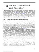
frequency response for this tweeter is shown in Figure 5.2. The 3-dB point below the
quoted 97 dB is at 4 kHz.
3588_C005.indd 105 11/20/07 4:22:25 PM
© 2008 by Taylor & Francis Group, LLC
106 Atmospheric Acoustic Remote Sensing
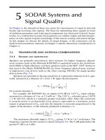
For the purposes of modeling performance, a good t to the angular patterns in
Figure 5.3 is obtained using I
max
cos
4
R, with I
max
=0.31, 1.9, 3.1, and 3.1Wm
–2
for
35 V
rms
at 1 m and for frequencies f
T
= 3.15, 4, 5, and 6 kHz. Integrating over the
forward hemisphere
2
2
5
4
0
2
PQQQ
P
P
II
max
/
max
cos sin d = 0.39, 2.4, 3.
°
99, and 3.9 W
for the total acoustic power. Measurements show that this speaker’s impedance at f
= 4 kHz is about 250 Ω, and is equivalent to a 0.12 µF capacitance in parallel with
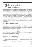
85 mm
120 mm
190 mm
FIGURE 5.1 Some speakers used in research SODARs. From left to right: Motorola
KSN1005, RCF 125/T, and Altec lansing 290-16L.
70
75
80
85
90
95
100
0 5 10 15 20
L
I
dB (2.83V
rms
@1m)
Frequency (kHz)
FIGURE 5.2 The measured frequency response of a Motorola KSN1005A speaker.
3588_C005.indd 106 11/20/07 4:22:28 PM
© 2008 by Taylor & Francis Group, LLC
SODAR Systems and Signal Quality 107
a 1 kΩ resistor (Figure 5.4). This means that the electrical power dissipated from
35 V
rms
input is 1.2 W. The electric-acoustic power conversion efciency is therefore
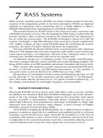
around 50% at 1 kHz. For monostatic use, this speaker is used as a microphone. Its
sensitivity was measured in comparison with a calibrated microphone, giving the
points in Figure 5.5.
Similar measurements can be performed on other speakers. The RCF 125/T is
quoted as having a 750 Hz cutoff and 120 dB re 1 V/1 m: its diameter is 120 mm.
The 290-16L has 3 dB cutoff at 300 Hz and a speaker diameter of 190 mm (but horn
diameter of 90 mm).
Note that the diameter of the speaker is related to its low-frequency 3 dB cutoff
frequency, as shown in Figure 5.6 for these three speakers.
Some speaker specications also quote their sensitivity as a microphone. For
example, the Four-Jay 440-8 has an output of 108 dB at 2 kHz for 1 W electrical
input into the 8 Ω, and a receiver sensitivity of 13.7 mV
rms
output for 1 Pa (i.e. L
I
= 94 dB) input. Note that sensitivity of
coil speakers is generally much less than
for piezoelectric speakers. These gures
can be compared with, for example, the
Knowles MR8540 microphone which has
a sensitivity of 6.3 µV for 1 Pa input.
From the combination of acoustic
power output as a speaker and voltage
input as a microphone, it is possible to
calculate the overall system gain V
micro-
phone
/V
speaker
for a single speaker or for an
90
120
150
180
210
240
270
300
330
0
30
60
1
0.8
0.6
0.4
0.2
FIGURE 5.3 Polar patterns of normalized intensity for the KSN1005 speaker at 3.15 kHz
(x), 4 kHz (dotted line), 5 kHz (*), 6 kHz (+), and cos
4
Ƨ (circles).
FIGURE 5.4 The equivalent electrical cir-
cuit for a KSN1005 speaker.
3588_C005.indd 107 11/20/07 4:22:30 PM
© 2008 by Taylor & Francis Group, LLC
108 Atmospheric Acoustic Remote Sensing
array. For example, with the KSN1005, 3 × 10
–4
Wm
–2
is obtained at 1 m for 1 V
rms
input, corresponding to 20 × 10
–6
(3×10
–4
/10
–12
) = 0.35 Pa. A KSN1005 placed at
1 m will record 0.1 × 0.35 = 0.035 V
rms
output. With a Four-Jay 440-8, 10
10.8–12
/8 =
7.9×10
–3
Wm
–2
or 1.8 Pa, giving 0.024 V
rms
output at an identical Four-Jay 440-8
at 1 m.
5.1.2 HORNS
All the speakers mentioned above have an acoustic horn connecting the driver ele-
ment to the atmosphere. The horn acts as an impedance-matching element from the
small-displacement high-pressure speaker diaphragm to a large-displacement lower-
pressure variation in the air. Horns generally have the diaphragm area larger than
the throat area: the ratio is called the compression ratio of the horn. For midrange
frequency the compression ratio is typically 2:1, and high-frequency tweeters can
have compression ratios as high as 10:1.
0
0.1
0.2
0.3
0.4
0.5
0.6
3456
Frequency (kHz)
Sensitivity (V/Pa)
FIGURE 5.5 Measured sensitivity of the KSN1005 used as a microphone.
1/f
T
= 0.03D – 2.2
0
1
2
3
4
50 100 150 200
Speaker Diameter D (mm)
1/f
T
(1/kHz)
FIGURE 5.6 The upper frequency 3 dB point for three speakers versus their diameter.
3588_C005.indd 108 11/20/07 4:22:32 PM
© 2008 by Taylor & Francis Group, LLC
SODAR Systems and Signal Quality 109
Information on horn design can readily be found in texts or web pages, but a
rough guide is that the length of the horn should be about the longest wavelength, M
L
,
which is going to be used, and the mouth of the horn should have a circumference
equal to or greater than M
L
. So for a 2-kHz system, the horn would be about 170-mm
long and 54-mm diameter. Horns generally have an exponential are, rather than
being conical, but for higher frequencies the shorter tractrix shape is common:
xrrr
xx x
ln ln( ) ,11 1
22
where x = (distance from the mouth)/(radius of the mouth) and r
x
=(radius at
distance x)/(radius of mouth) – in other words dimensions are scaled by the mouth
radius which is typically M
L
/2π.
The beam pattern from a horn having a mouth radius a is again just the pattern
from a hole of radius a,
P
Jka
ka
s
§
©
¨
¨
·
¹
¸
¸
2
1
2
sin
sin
.
Q
Q
5.1.3 PHASED-ARRAY FREQUENCY RANGE
The beam polar pattern is the product of the speaker polar pattern and the array
or dish pattern. The individual speaker pattern changes with frequency: Figure 5.7
shows the measured pattern for a single KSN1005 at 4 and 6 kHz. It is clear that the
array pattern will dominate over the small changes in the individual speaker pattern.
–45
–40
–35
–30
–25
–20
–15
–10
–5
0
FIGURE 5.7 Polar patterns for an individual KSN1005 at 4 kHz (solid line) and 6 kHz
(dashed line).
3588_C005.indd 109 11/20/07 4:22:35 PM
© 2008 by Taylor & Francis Group, LLC
110 Atmospheric Acoustic Remote Sensing
The rst minimum from an array consisting of M × M speakers separated by
distance d is given by Eq. (4.8) as ∆R≈c/Mdf
T
, so for reasonably large arrays the
beam width is inversely proportional to frequency. A more narrow and intense beam
is desirable. Eq. (4.3), giving the rst two side lobe zenith angles R
L
on either side of
the main beam, can be expressed in the form
sin ,Q
L
TT
3
4
5
4
c
fd
c
fd
(5.2)
if an incremental phase shift of π/2 is used. If the next main lobe is kept below a
zenith angle of 45°, 34 12cfd
T
//
. If beams are directed at 45° to rows or col-
umns of close-packed speakers, then d can be replaced by d/ 2 . A useful guide
based on the second lobe position and the relationship between speaker efciency
and its diameter (in m) is therefore
cfd
T
/2 1
and f
T
> 1000/(30d−2.2), or
1000
30 2 2
3
2d
d
c
fd
c
T
.
(5.3)
For example, for the KSN1005, this gives 3 kHz < f
T
< 6 kHz. Extensive eld
tests with the AeroVironment 4000 have proven these to be practical limits.
5.1.4 DISH DESIGN
As an example of a dish antenna design, Figure 5.8 shows a 3-beam system based
on the Four-Jay 440-8 re-entrant cone speaker and a 1.2-m dish. Figure 5.9 shows
the measured beam patterns. The half-width at −3 dB (a common measure) is 25° for
the speaker and 6° for the antenna plus dish, showing the focussing effect described
1200 mm
133 mm
220 mm
72
180
210
240
270
300
330
150
120
90
40
30
20
60
30
0
410 mm
25
FIGURE 5.8 The design of a dish-based 3-beam system.
3588_C005.indd 110 11/20/07 4:22:41 PM
© 2008 by Taylor & Francis Group, LLC
SODAR Systems and Signal Quality 111
earlier. Note that diffraction effects can easily be seen past about 25° for the dish
system. Figure 5.10 shows a spun aluminum dish. In this prototype, the distance of
the speaker from the dish can be adjusted, since the equivalent source point within
the speaker horn is not known.
5.1.5 DESIGNING FOR ABSORPTION
AND
BACKGROUND NOISE
Obviously absorption is lower at lower frequencies. The absorption is of order
0.003f
kHz
2
dB m
–1
at 50% relative humidity and 10°C. Roughly speaking, the differ-
ence between f
T
= 2 and 6 kHz is an extra 10 dB lost per 100 m. This is a lot.
From Chapter 3, background noise decreases roughly as
f
T
q
, so higher trans-
mitting frequencies are favored. But since background noise depends on a power of
f
T
and absorption depends on the exponential of frequency-dependent absorption
times range, there will be an optimum frequency for any given range. The ratio of
received signal power to received acoustic noise power (SNR) is written as
SNR
A
fz
f
Af bf z
q
q
T
T
T
T
13
13 2
2
2
/
/
exp
exp(
|
)),
(5.4)
so
–35
–30
–25
–20
–15
–10
–5
0
–50 –40 –30 –20 –10 0 10 20 30 40 50
Zenith Angle (degrees)
Normalised Gain (dB)
FIGURE 5.9 Measured beam patterns for the dish system at 3 kHz: speaker pattern with-
out dish (line with dots); speaker at calculated focal distance (solid line); speaker at other
positions within ±50 mm of the calculated focus.
3588_C005.indd 111 11/20/07 4:22:44 PM
© 2008 by Taylor & Francis Group, LLC
112 Atmospheric Acoustic Remote Sensing
dSNR
df
A
q
f
bzf f bf
q
TT
T
T
T
§
©
¨
¨
·
¹
¸
¸
13
42
2
/
exp( zz)
and the optimal f
T
for a xed range z is
f
q
bz
T
13
4
/
(5.5)
The slope of the background noise spectrum for the daytime city is about q = 2.8
so for a range of z = 1000 m, given b = 0.003/10 log
10
e = 7×10
–4
m
–1
, the optimum
f
T
= 1 kHz. In practice this is a little pessimistic, since good signal processing can
extend the optimum frequency by about a factor of 2, as shown in Figure 5.11.
5.1.6 REJECTING RAIN CLUTTER
Scattering from rain depends on
f
T
4
, so lower frequencies give markedly less spec-
tral noise from rain. For example, the SNR in rain will be around 20 dB better at f
T
= 2 kHz than at 4.5 kHz: high-frequency mini-SODARs have real problems during
rain! However, acoustic noise from drop splashing is likely to be greater at lower
frequencies.
Figure 5.12 shows measurements taken on ve different roong panel structures
(Hopkins, 2004). These comprise: 25-mm thick polycarbonate sheet (ve layers of
3.4kgm
–2
); laminated glazing (6-mm toughened glass, 12-mm air space, 6.4-mm
laminate glass); and ETFE pillows of a 150-micron layer taped to a 50-micron layer
with a 200-mm air gap with and without two types of rain suppressors. The rain
noise in all cases decreases as f
–3/2
. This means that the overall effect of rain, con-
sidered as a noise source, varies as
f
T
52/
, so that lower frequency SODARs perform
better.
FIGURE 5.10 A dish antenna system.
3588_C005.indd 112 11/20/07 4:22:49 PM
© 2008 by Taylor & Francis Group, LLC
SODAR Systems and Signal Quality 113
1200
1000
800
600
Range (m)
400
200
0
123
Optimum Transmit Frequency (kHz)
4567
FIGURE 5.11 The optimum transmit frequency for a given range, determined by the
balance between decreasing background noise and increasing absorption with increasing
frequency.
# !"
! L
I
'
%$&
FIGURE 5.12 Spectral intensity levels measured on ETFE (circles), polycarbonate (x),
ETFE with rain suppressor type 1 (squares), ETFE with rain suppressor type 2 (triangles), and
laminated glazing (+). Also shown is a curve having an f
–3/2
dependence (black diamonds).
3588_C005.indd 113 11/20/07 4:22:51 PM
© 2008 by Taylor & Francis Group, LLC
114 Atmospheric Acoustic Remote Sensing
5.1.7 HOW MUCH POWER SHOULD BE TRANSMITTED?
The answer is, of course, as much as possible within the limitations of the speak-
ers. There have been some massive low-frequency SODARs built, but they have
little popularity because of their bulk, their need for high electrical power, and their
obtrusive environmental noise.
The Scintec combination of small (SFAS), medium (MFAS), and large (XFAS)
phased-array SODARs uses similar technology and is a good indication of cost/ben-
et versus power (see Table 5.1 and Figure 5.13).
TABLE 5.1
Characteristics of the Scintec range of SODARs
SFAS MFAS XFAS
P
acoustic
(W) 2.5 7.5 35
P
12 V
(kW) 0.1 0.2 0.7
Diameter (m) 0.42 0.72 1.45
Volume (m
3
) 0.03 0.1 0.7
Mass (kg) 11.5 32 144
f
T
(kHz) 3.2 2.2 1.0
z
min
(m) 10 20 20
z
max
(km) 0.5 1 2
0
1
2
3
4
1 10 100
Diameter (m), Frequency (kHz), Range (km)
Power (W)
FIGURE 5.13 Characteristics of the Scintec SODARs. Diameter (circles), transmit fre-
quency f
T
(squares), and claimed maximum range (triangles).
3588_C005.indd 114 11/20/07 4:22:52 PM
© 2008 by Taylor & Francis Group, LLC
SODAR Systems and Signal Quality 115
5.2 SODAR TIMING
5.2.1 P
ULSE SHAPE, DURATION, AND REPETITION
SODARs generate a pulse which has the generic shape shown in Figure 5.14. The
key parameters are transmit frequency f
T
, pulse period U, and ramp up/down time
CU. Transmission of such pulses is repeated with pulse repetition rate T as shown in
Figure 5.15.
Because there are multiple beams in a monostatic system, the pulse repetition
rate for an individual beam will be the number of beams times the repetition rate
for transmitting. The power transmitted is proportional to the pulse length U, for a
given pulse amplitude. Also, the Doppler spectrum frequency resolution is better
with a longer pulse. This can be visualized by estimating f
T
by counting the number
of cycles, n, in time U, and then
f
n
T
T
If there is a ±1 uncertainty in n, then the uncertainty in f
T
is
$f
T
o
1
T
(5.6)
The spectral line from a constant Doppler shift is therefore spread to 2/U wide. The
practical Doppler resolution is actually better than this because of averaging and peak-
detection schemes, as discussed later, but the spectral width is still a basic limitation.
However, a longer transmitted pulse means a longer range gate and poorer spa-
tial resolution. Basically two layers cannot be distinguished if they are within verti-
cal distance cU/2 of each other.
f
T
FIGURE 5.14 The generic shape of SODAR pulses of duration Ʋ.
FIGURE 5.15 The repetition of pulses in a SODAR system.
3588_C005.indd 115 11/20/07 4:22:56 PM
© 2008 by Taylor & Francis Group, LLC
116 Atmospheric Acoustic Remote Sensing
A practical compromise seems to be U~ 30 to 80 ms, giving f
T
~ 10 to 30 Hz,
or (raw) uncertainty in horizontal wind speed of 1 to 3 m/s, and spatial resolution of
5 to 14 m.
The pulse repetition rate, T, is determined by the highest range z
T
from which
echoes are expected. It is important that this is chosen conservatively (i.e., pick a
much larger T than the range of interest), otherwise echo returns from higher than
this range, from an earlier pulse, will add to those from lower down due to the
current pulse. This means that echo returns are combined from heights ct/2 and
c(t+T)/2. For example, the AeroVironment 4000 typically has T = 1.33 s, giving z
T
=
340 ì 1.33/2 = 220 m, for the 200 m typically analyzed.
It is desirable to shape the start and end of the pulse as shown, since this reduces
oscillations in the frequency spectrum, and consequently limits spreading of power
from a spectral peak into adjacent spectrum bins. To do this, the pulse voltage is
typically multiplied by a Hanning shape
mt
t
Ô
Ư
Ơ
Ơ
Ơ
Ơ
ả
à
à
à
à
Đ
â
ă
ă
ă
ã
ạ
á
á
á
1
2
10cos
P
BT
for tt
t
t
[]
Ô
Ư
Ơ
Ơ
Ơ
Ơ
ả
BT
BT T B
P
BT
T
11
1
2
1
for
cos
àà
à
à
à
Đ
â
ă
ă
ă
ã
ạ
á
á
á
ê
ô
ơ
for TB T1 t
(5.7)
or a Gaussian shape
mt
et
t
m
t
1
2
2
2
0
11
S
BT
BT
BT T B
for
for
eet
m
t
[]
ê
ô
1
2
1
2
2
1
S
BT
TB Tfor
ơ
(5.8)
These have Fourier transforms of
Mf f f
f
f
Đ
â
ă
ã
ạ
á
TPT B PTB
PT
PT
sin cos1
11
2 11
1
21//BPT B
Đ
â
ă
ă
ă
ã
ạ
á
á
á
f
(5.9)
and
Mf
f
f
f
() *
sin( )
,
(/ )
1
2
12
22
PS
PT
PT
S
f
e
f
(5.10)
3588_C005.indd 116 11/20/07 4:23:01 PM
â 2008 by Taylor & Francis Group, LLC
SODAR Systems and Signal Quality 117
where
*
means the convolution product and T
f
= 1/(2QT
m
). Pulse envelopes are shown
in Figure 5.16 and their corresponding spectra in Figure 5.17.
It is clear from Figure 5.17 that a smoother pulse envelope produces a smoother
and wider spectrum. The smoothness is desirable, since it reduces the possibility of
secondary maximum adding to noise to give a spurious Doppler peak estimate and
hence a false wind estimate. On the other hand, a wider spectrum makes it more
difcult to estimate the point of highest curvature (the spectral peak position). In all
cases, the spectral shape can be estimated by a Gaussian of width T
f
in the central
region. For the Hanning case,
ST B
f
052 073 (5.11)
and for the Gaussian case with T
m
= U/4,
ST
f
064 (5.12)
5.2.2 RANGE GATES
The received signal depends on the convolution of the atmospheric turbulent scat-
tering cross-section prole with the pulse envelope, as expressed in (4.33). For the
zero-Doppler case,
pt zmt t ft t z
zzRs T
() ()()exp[()].| SP
°
jd2
0
∞
The pulse shape m(t) and duration U determine spatial resolution of the SODAR
through this term. Spatial resolution is the vertical separation ∆z
m
of two innitely
0.0
0.2
0.4
0.6
0.8
–0.5 –0.3 –0.1 0.1 0.3 0.5
Normalised Time
Amplitude
1.0
FIGURE 5.16 Pulse envelopes for a Gaussian with T
m
=U/4 (dark solid line), Hanning with
C = 0.2 (light line), and Hanning with C = 0.5 (dashed line).
3588_C005.indd 117 11/20/07 4:23:05 PM
© 2008 by Taylor & Francis Group, LLC
118 Atmospheric Acoustic Remote Sensing
thin layers which is resolved in the returned signal. Two peaks in the time series are
resolved if the signal drops to at least half power between them. If T
s
consists of delta
functions at heights z
1
and z
2
, then
pt zz zzmt
z
c
R
() [( ) ( )] ex| DD
Ô
Ư
Ơ
Ơ
Ơ
Ơ
ả
à
à
à
à
12
2
pp
Ô
Ư
Ơ
Ơ
Ơ
Ơ
ả
à
à
à
à
Ô
Ư
Ơ
Ơ
Ơ
Ơ
jd2
2
2
0
1
Pf
z
c
z
mt
z
c
T
|
ảả
à
à
à
à
Ô
Ư
Ơ
Ơ
Ơ
Ơ
ả
à
à
à
à
Ô
Ư
Ơ
Ơ
exp j2
22
12
Pf
z
c
mt
z
c
T
ƠƠ
Ơ
ả
à
à
à
à
Ô
Ư
Ơ
Ơ
Ơ
Ơ
ả
à
à
à
à
exp ,j2
2
2
Pf
z
c
T
which has an envelope of
mt
z
c
mt
z
c
Ô
Ư
Ơ
Ơ
Ơ
ả
à
à
à
à
Ô
Ư
Ơ
Ơ
Ơ
ả
à
à
à
à
22
12
.
For the Gaussian case, if z
2
= z
1
+z
m
, then the minimum of the combined enve-
lope pattern occurs at t = (2z
1
/c +2z
2
/c)/2 or t2z
1
/c =z
m
/c and t2z
2
/c =z
m
/c. The
situation is shown in Figure 5.18. At this time, the peaks are resolved if
2
1
2
1
2
2
2
exp
Ô
Ư
Ơ
Ơ
Ơ
Ơ
ả
à
à
à
à
Đ
â
ă
ă
ă
ã
ạ
á
á
á
a
S
m
m
z
c
$
or
$zc
mm
qS ln .8
(5.13)
0.2
0.0
0.2
0.4
0.6
0.8
1.0
8 6 4 2 0 2 4 6 8
Normalised Frequency
Amplitude
FIGURE 5.17 Frequency spectra corresponding to a Gaussian envelope with
m
= /4 (dark
solid line), a Hanning envelope with = 0.2 (light line), and a Hanning envelope with = 0.5
(dashed line).
3588_C005.indd 118 11/20/07 4:23:11 PM
â 2008 by Taylor & Francis Group, LLC
SODAR Systems and Signal Quality 119
For T
m
= U/4, ∆z
m
>0.36cU. For a square pulse envelope, ∆z
m
>0.5cU for two spa-
tial features to be resolved.
This spatial resolution for turbulence measurements is determined by the pulse
shape. In practice, the SODAR will usually sample much more rapidly than this, but
this does not increase spatial resolution.
More importantly for many applications is the spatial scale resolved for wind
vectors. Wind components are estimated from the Doppler shift in the peak power
in a power spectrum. Each power spectrum is obtained from a Fourier transform of
a set of M data values sampled at time intervals of ∆t. This means that wind compo-
nent estimates are only obtained from height intervals of
$
$
z
cM t
c
V
()
(5.14)
Again, SODARs will often present results at ner spatial resolution, perhaps by
doing fast Fourier transforms (FFTs) using overlapping sequences of samples. While
this may look good on a prole plot, no extra information is contained.
For example, assume that a 2 kHz SODAR has pulse length
U = 50 ms, and the
atmosphere has c= 340ms
–1
, a constant T
s
, and Doppler shift of −45 Hz below z
0
=
85 m and +45 Hz above that level. The recorded time series consists of a pure sine
wave at 1960 Hz for the rst 0.5 s, a mixture of 1960 and 2040 Hz until 0.55 s, and
then a pure tone at 2040 Hz. The signal is sampled at
f
s
= 960 Hz for M = 64 points,
producing samples at frequencies 960/64 = 15 Hz apart.
The spatial resolution due to the FFT length is ∆z
V
= 11.3 m and that due to pulse
length is ∆z
m
= 8.5 m. Spectral resolution due to the nite sampling length of T =
M/f
s
= 67 ms is 1/T = 15 Hz (the rst zeros of the spectrum are at 45±15 Hz). If the
nite pulse length is included, the spectral resolution is now 1/U = 20 Hz. In fact the
pure tone spectral line is convolved with both the spectrum from the nite sampling
0
0.2
0.4
0.6
0.8
1
1.2
–1.5 –1.0 –0.5 0.0 0.5 1.0 1.5
Normalised Time
Amplitude
FIGURE 5.18 The combination of two Gaussian envelopes which allows spatial features
to just be resolved.
3588_C005.indd 119 11/20/07 4:23:13 PM
© 2008 by Taylor & Francis Group, LLC
120 Atmospheric Acoustic Remote Sensing
length and the spectrum from the nite pulse length. Convolving the spectrum is
equivalent to multiplying the time series by a rectangular function. In this case the
time series is being multiplied by two rectangular functions, and this is equivalent to
simply multiplying by the shorter rectangle. So the spectral resolution is determined
by the shorter of T and U.
To summarize spatial and spectral resolutions:
Spatial resolution for turbulence:
$z
c
m
T
2
,
Spatial resolution for winds:
$z
V
the larger of
cT
2
and
cM
f2
s
,
Wind speed spectral resolution:
%f
V
=the larger of
f
M
s
and
1
T
,
Wind speed resolution:
V = the larger of
cf
Mf
s
T
2
and
c
f
T
2T
Uncertainty product for winds:
T
s
$$zV
c
f
f
V
2
4
TTT
T
M
f
M
c
f
f
M
Ô
Ư
Ơ
Ơ
Ơ
ả
à
à
à
Ô
Ư
Ơ
Ơ
Ơ
ả
à
à
à
1
2
1
4
if
s
T
s
,
iif
s
1
ê
ô
ơ
f
M
T
.
From the above it is clear that the minimum of the resolution product is when U
= M/f
s
= T. Then
$$zV
c
f
V
T
2
4
(5.15)
Typically, c = 340ms
1
and f
T
= 4000 Hz, so z
V
V 7 m
2
s
1
. If z
V
= 10 m,
then V = 0.7ms
1
. This is a good rst guide, but later it will be seen that good peak
detection and averaging can improve velocity resolution substantially.
5.3 BASIC HARDWARE UNITS
5.3.1 T
HE BASIC COMPONENTS OF A SODAR RECEIVER
All SODAR receivers consist of some common components: microphones to convert
acoustic power into electrical power; ampliers to provide large enough voltages for
digital processing; lters to reject unwanted noise; and digitization modules.
5.3.2 MICROPHONE ARRAY
Most SODARs are monostatic, so use the speaker as a microphone. This precludes
using a sensitive microphone. Horn speakers are generally used, where the small
speaker driver is impedance matched to the atmosphere via a horn-shaped extension.
A typical phased array made of 64 of the 0.085-m square KSN1005 speakers will
have an area of 64 ì 0.085 ì 0.085 = 0.46 m
2
and an equivalent radius of a ~0.4 m.
3588_C005.indd 120 11/20/07 4:23:23 PM
â 2008 by Taylor & Francis Group, LLC
SODAR Systems and Signal Quality 121
The power received from turbulence at 100 m is of order 10
–14
GA
e
, or ~10
–14
W, giving
an intensity of 10
–14
/0.46~2 × 10
–14
Wm
–2
at 1 m. Normal microphone sensitivities
vary from about −20 dB referred to 1 V/Pa (or 0.1 V/Pa) for a carbon microphone, to
−90 dB re 1 V/Pa for a ribbon microphone. Sound pressure is approximately
30 I
Pa for intensity I in Pa, or about 4 µPa from the turbulence. This means that normal
microphones will give from about 10
–12
to 10
–7
V
rms
output.
The voltage produced by the piezoelectric KSN1005, acting as a microphone,
should be around 10
–8
V
rms
, or 0.6 µV
rms
for the whole array.
Moving coil speakers are also commonly used for lower-frequency SODARs.
Moving coil microphones are typically two orders of magnitude less sensitive than
piezomicrophones, but the atmospheric absorption coefcient is almost an order of
magnitude smaller for a 1.6 kHz system compared to a 4.5 kHz system. The result is
perhaps an order of magnitude smaller signal, say 60 nV
rms
.
Note that with such small signals, some care is necessary with electrical shield-
ing and grounding.
5.3.3 LOW-NOISE AMPLIFIERS
Typical outputs from the speaker/microphone array are 100 to 1000 nV
rms
, so around
120 dB voltage gain (10
6
) is required in the receiver to produce signals in the vicin-
ity of 1 V for digitization. In practice, the microphone/speaker self-noise and other
external acoustic noise will generally be larger (meaning some signal averaging will
be needed), but a good design goal would be to minimize that component of the noise
over which the designer has control. The equivalent RMS noise voltage in a 100 Hz
bandwidth at the input of a good low-noise operational amplier is 10 nV, about 10%
of the expected input signal, so it is important to choose the preamplier carefully
and to take care with circuit layout and ground connections. It is also important to
keep input resistance small, so that resistor noise does not contribute signicantly.
As an example, a common low-noise op-amp is the AD OP-27E, having 3 nV Hz
–1/2
noise at its input. For 100 Hz bandwidth this gives 30 nV noise at the input. A gain of
1000 (60 dB) can readily be used with this op-amp, using say 10Ω input resistors and
10 kΩ feedback resistors, as shown in Figure 5.19.
Resistor noise can be reduced further using parallel resistors, since the resistor
noise in each resistor is uncorrelated, whereas the input currents from the desired
FIGURE 5.19 $W\SLFDOSUHDPSOLÀHULQSXWVWDJH
3588_C005.indd 121 11/20/07 4:23:25 PM
© 2008 by Taylor & Francis Group, LLC
122 Atmospheric Acoustic Remote Sensing
signals are correlated. For example, if s
1
and s
2
are two signals with the same signal
mean and same (uncorrelated) noise levels:
ss ss s
T
ss ss
ss
12 12
2
12 12
2
1
12
§
©
¨
·
¹
¸
S
22
0
11 2 2
2
0
1
1
1
dt
T
ss ss dt
T
s
T
T
°
°
§
©
¨
·
¹
¸
ssdt
T
ssssdt
T
ss
TT
1
2
0
1122
0
22
21
°°
22
0
11
2
0
22
2
0
11
1
dt
T
ssdt
T
ssdt
T
TT
s
°
°°
S
222 2
2
2
2
2
2
1
2
SS
S
S
ss
s
s
SN R
ss
(5.16)
so the SNR decreases by 1/M
1/2
for M signals added together. This is a particularly
useful technique for phased arrays consisting of many speakers/microphones. For
example, an array of 64 microphones will have an SNR improvement of a factor of
8 in amplitude or 18 dB in power. Some ltering can also be usefully done at this
point, by including capacitors across each of the two 10 kΩ resistors.
5.3.4 RAMP GAIN
Since the echo signal decreases with distance (and therefore time) due to beam
spreading and absorption, it is convenient to include a ramped gain stage in the
receiver. This can be achieved by using an analog multiplier (MLT04 or equivalent)
which has an output which is the product of the input and a gain signal. The gain
signal can be generated by the SODAR computer as an 8-bit or 10-bit code converted
to analog form via an 8-bit or 10-bit digital to analog convertor (DAC). Usually
the gain signal will simply increase linearly with time (received power is inversely
proportional to the square of distance or time, so received amplitude is proportional
to the inverse of distance or time). However, more recent SODAR designs simply
digitize the signal at very high resolution (24 bits) and at a lower receiver gain, so that
there is enough dynamic range, without running out of voltage range for the larger
signal+noise signals, while still recording the faintest signal components at sufcient
resolution. In these designs, all processes such as ltering and ramp gain are done in
3588_C005.indd 122 11/20/07 4:23:27 PM
© 2008 by Taylor & Francis Group, LLC
SODAR Systems and Signal Quality 123
software, as well as allowance for absorption, depending on measured temperature
and/or humidity.
5.3.5 FILTERS
Random electronic noise can easily be 30% of the signal received from 100 m. Hard-
ware lters can be used to improve this SNR. Generally a relatively simple band-pass
lter might follow the preamplier. The bandwidth (BW) required is the maximum
Doppler shift
$f
V
c
f
2
max
sin
.
J
T
(5.17)
Typically the maximum wind speed capability is 25 m s
–1
(at which speed wind
noise is often signicant), and the beam tilt angle is ~20°, so the required Q of the
BP lter is
Q
f
f
T
y
$
20
(5.18)
(the Q factor is a measure of a lter’s selectivity). Typically a 4-pole pair BP
lter with Q = 10 to 20 would be used at this stage, and might have a gain of 10
(i.e., 20 dB). This could be a unit purchased as a complete module, or comprise
an active lter IC and some tuning components, or be built up from op-amps.
It could also be a digitally programmable lter if it were desired to be able to
change f
T
. Programmable lters can be based on ICs such as the LTC1068 which
requires a tuning input at 100 or 200 times the desired center frequency. Modu-
lar programmable BP lters are also available, such as the Frequency Devices
828BP which has an 8-bit parallel programmable center frequency. Typical val-
ues are given in the circuit of Figure 5.20, with a voltage transfer function shown
in Figure 5.21 for a 2-kHz SODAR. The output from the lter will have noise
reduced by a factor of 10 in comparison with the signal.
5.3.6 MIXING TO LOWER FREQUENCIES (DEMODULATION)
In practice, all the useful information is contained in the signal amplitude and in the
Doppler shift, so any pure signal component at frequency f
T
can be removed. The
"
%
%
%
%
!$
#
FIGURE 5.20 7KHHIIHFWRIDEDQGSDVVÀOWHUVWDJH
3588_C005.indd 123 11/20/07 4:23:30 PM
© 2008 by Taylor & Francis Group, LLC
124 Atmospheric Acoustic Remote Sensing
mixing process can be understood from the plot in Figure 5.22 of a modulated echo
signal (top trace). The second trace shows the mixing signal which is multiplied with
the echo signal. This produces the third trace. Finally, a simple low-pass lter, such
as provided by an RC circuit, produces the smoothed bottom trace. This last trace
contains the modulation signal.
This demodulation can be accomplished with an analog multiplier IC, such
as the Analog Devices MLT04, or by switching between the signal and ground at
the mixing frequency using an analog switch IC. The mixer is then followed by
an LP lter to remove the higher frequencies, as shown in the complete circuit of
Figure 5.23.
Time (ms)
0123 45 6
FIGURE 5.22 Demodulation of a modulated signal (upper trace) by multiplying with a
mixing signal (second trace from the top) to give a composite low-frequency and 2f
T
signal
(third trace) which can be low-pass ltered to give the modulation (bottom trace).
FIGURE 5.21 A typical voltage transfer function for a band-pass lter.
3588_C005.indd 124 11/20/07 4:23:32 PM
© 2008 by Taylor & Francis Group, LLC
0
–20
–40
–60
–80
–100
–120
2 kHz
10 1 kHz 0.2
Frequency (Hz)
Normalised Gain (dB)
SODAR Systems and Signal Quality 125
It is seen that the initial power SNR of 20 log
10
(1 mV/0.3 mV) = 10 dB has been
increased to 20 log
10
(1 V/0.01 V) = 40 dB.
Similarly, FM modulation produced by Doppler shift will be demodulated using
this mixer, as shown in Figure 5.24. Of course, the modulation is in practice of much
lower frequency than the transmitted frequency, and a sharp cutoff LP lter gives a
much smoother output than shown in the gure.
For this example, it can be seen that the mixing frequency is 4.5 kHz. From the
FM demodulated (low frequency) traces, the period of the Doppler component is
seen to be about 2.2 ms (∆
f = 450 Hz). The in-phase mixed demodulated signal lags
the 90°-phase demodulated signal by 90°. This is a case of positive Doppler shift,
with the raw signal frequency being 4.95 kHz.
If, on the other hand, the raw signal frequency is 4.05 kHz, the in-phase trace
is the same as in Figure 5.24, but the 90°-phase trace is inverted, and the in-phase
mixed demodulated signal leads the 90°-phase demodulated signal by 90°. This is
a case of negative Doppler shift. So it can be seen that the relative phase of the
in-phase and 90°-phase demodulated signals shows whether the wind component is
toward the SODAR (positive shift) or away from the SODAR (negative shift).
" !
f
dt
t
dV
FIGURE 5.23 The complete amplier and lter chain.
Time (ms)
0123456
Time (ms)
0123456
FIGURE 5.24 Demodulation of a Doppler-shifted (FM) signal. Mixing with a square wave
in phase with the original transmitted signal is shown on the left, and mixing with a quadra-
ture phase (90° phase-shifted) square wave on the right.
3588_C005.indd 125 11/20/07 4:23:35 PM
© 2008 by Taylor & Francis Group, LLC
126 Atmospheric Acoustic Remote Sensing
The signal is generally mixed down to a lower frequency. The mixer stage will
be followed by a low-pass (LP) lter. Again this could be programmable and/or mod-
ular. This lter’s transfer function could be similar to that shown in Figure 5.25.
5.3.7 SWITCHING FROM TRANSMIT TO RECEIVE, AND ANTENNA RINGING
The monostatic SODAR uses the same transducer to transmit and receive. This
requires switching the speaker from its connection to a power amplier so that it is
connected as a microphone to the sensitive preamplier. This switching should be
done as rapidly as possible after the end of the transmitted pulse, so that echoes from
low altitudes can be analyzed.
There are a number of problems associated with this switching. First, the switch
must be an analog switch (i.e., allow continuously varying signals to pass through
it). Secondly, it must handle relatively high voltages and currents during transmitting
(of order 100 V into 16 Ω for a coil speaker, giving 6 A), as well as the very small volt
-
ages and currents during receiving (of order 1 µV into 10 Ω, giving 100 nA). Switching
should be stabilized after the equivalent of a few meters of pulse travel (say 20 ms). In
addition, there must be very good isolation of the preamplier from the power ampli-
er, and care must be taken that transients do not destroy the preamplier.
In spite of these difculties, a simple relay such as the Omron G2RL has a current
rating of 8 A, a turn-on time of 7 ms, and a turn-off time of 2 ms, and will be suf
-
cient. More sophisticated semiconductor switches (TRIACs, etc.) can also be used.
The real problem with recording useful data at a low altitude is that the antenna
and the bafe enclosure are likely to “ring” for some time after the transmit pulse.
This is not simply the time taken for sound to travel along the bafe and back to
the speakers, since a typical speed in a composite wooden bafe might be 10
3
ms
–1
and for a length of 2 m this would only give a return time of 4 ms. The problem is
reverberation time of both the bafes and the speaker enclosure. A good design
will attempt to damp any reverberations. This can be approached by using “soft”
materials for the bafe, such as composite wood, perhaps coated with a matting or
lead layer, and by lling the speaker enclosure with acoustic foam and perhaps other
“deadening” materials. Even so, the problems with reverberations are likely to affect
0
10
Attenuation (dB)
–10
–20
–30
–40
–50
–60
–70
–80
–90
10 100
Frequency (Hz)
1000 10000
–800
–700
–600
–500
–400
–300
–200
–100
Phase (deg.)
0
–100
FIGURE 5.25 7KHJDLQDQGSKDVHRIDW\SLFDO/3ÀOWHU
3588_C005.indd 126 11/20/07 4:23:36 PM
© 2008 by Taylor & Francis Group, LLC
SODAR Systems and Signal Quality 127
data quality for at least the lowest 6 to 10 m (40 ms). Figure 5.26 shows a typical
transient from an AeroVironment 4000 SODAR.
The SODAR settings for this example were 100% amplitude and 60-ms pulse
length. Generally it is to be expected that more power and longer pulse lengths will
increase reverberation. Protecting the preamplier input from transients, such as
reverberations, is simply a matter of installing protecting diodes across all resistors
and the input of the preamplier. Genuine echo signals will always be sufciently
small that these diodes will not be turned on.
5.4 DATA AVAILABILITY
5.4.1 T
HE HIGHEST USEFUL RANGE
A 2-kHz SODAR might range to, say, 400 m, and a typical 4.5 kHz system might
range to 200 m at a quiet country daytime site (of course depending on turbulence
intensities). At these heights the SNR will be around 1. Most of the difference in
range capability will be due to absorption dependence on frequency. The absorption
coefcients are, for 50% relative humidity and at 10°C, B≈ 0.01 dB/m (0.002 m
–1
) at
2 kHz, and B≈ 0.05 dB/m (0.01 m
–1
) at 4.5 kHz. From Chapter 3, the frequency- and
range-dependent terms in the SNR are, from the SODAR equation,
f
e
z
q
z
1
3
2
2
A
(5.19)
and the ratio of these for the two frequencies and ranges is of order 1. However,
as seen in Chapter 3, the noise dependence on frequency, q, is about 2.8 for city
backgrounds, 1.4 for daytime country, and 0.5 for nighttime country. Combining
these concepts allows an estimate of SNR versus SODAR frequency, depending on
site background noise. This is plotted in Figure 5.27, assuming constant backscatter
with height, independent of site and time of day. The turbulence levels vary substan-
tially, but, for example, if a z
-4/3
dependence for
C
T
2
is assumed (as found by various
groups for convective boundary layers) then the SNR would fall off more rapidly
with height.
0
500
1000
1500
2000
2500
3000
0 20406080100120
Time (ms)
Voltage (mV)
FIGURE 5.26 Signal amplitude levels recorded from an AeroVironment 4000 SODAR
ZLWKLQWKHÀUVWPVIROORZLQJWKHWUDQVPLWSXOVH
3588_C005.indd 127 11/20/07 4:23:39 PM
© 2008 by Taylor & Francis Group, LLC
128 Atmospheric Acoustic Remote Sensing
5.5 LOSS OF SIGNAL IN NOISE
One of the principal problems of ground-based remote sensing is the poorer data
availability at greater heights, and the fact that data availability depends on meteo-
rological conditions. The SODAR equations can be written as
PP P P P
AFPN
,
(5.20)
Night Time City
Night Time Country
Frequency (kHz)
Height (m)
1000
900
800
0
0
20
20
40
–40
–40
–20
–20
–60
–60
700
600
500
400
300
200
100
1 1.5 2 2.5 3 3.5 4 4.5 5 5.5 6
Frequency (kHz)
Height (m)
1000
900
800
700
600
500
400
300
200
100
1 1.5 2 2.5 3 3.5 4 4.5 5 5.5 6
FIGURE 5.27 SNR versus height and frequency for night time country environments
(upper plot), night-time city environments (middle plot), and daytime city environments
(lower plot).
3588_C005.indd 128 11/20/07 4:23:41 PM
© 2008 by Taylor & Francis Group, LLC
SODAR Systems and Signal Quality 129
where P is the total received power, P
A
is the power scattered from atmospheric
turbulence, P
F
the power reected from xed objects such as masts, P
P
the power
scattered from precipitation, and P
N
noise power. The required signal is from P
A
and
the remaining terms on the right lead to reduced SNR = P
A
/(P
F
+P
P
+P
N
).
Generally P
F
may be reduced by selecting the orientation of the SODAR to mini-
mize power transmitted toward the xed object. If P
F
is still present, then it can often
be identied because it has zero Doppler shift and its spectral width may be different
from that of P
A
. While xed echoes remain an operational problem, for calibration
purposes and even in many data collection applications, those range gates affected
can simply be ignored.
Echoes from precipitation are also an operational problem for SODARs, but these
data can effectively be eliminated because the presence of rainfall can be sensed via
other means or from the increased vertical velocities detected by the SODAR.
External noise remains the main difculty during calibration. Both P
A
and P
N
can be variable. From the SODAR equation
PPGAf
c
Tz
z
ATeT
r
§
©
¨
¨
·
¹
¸
¸
[]
/
/
310
413
23
2
2
2
T
A
e
§§
©
¨
¨
·
¹
¸
¸
C
T
2
. (5.21)
The rst square bracket contains factors determined by the instrument, and the sec-
ond square bracket contains terms only weakly dependent on atmospheric tempera-
ture prole variations. The third square bracket contains terms representing signal
loss due to absorption and spherical spreading, and the
C
T
2
term represents the echo
signal generation. The absorption is generally not very large, so most signal loss
is through the unavoidable inverse-square reduction with height. For example, the
inverse square loss between 10 and 100 m is 20 dB, whereas the absorption loss is
around 0.6 dB for a 1 kHz SODAR and 6 dB for a 4.5 kHz SODAR.
Day Time City
Frequency (kHz)
Height (m)
1000
900
800
0
–20
–60
–40
700
600
500
400
300
200
100
1 1.5 2 2.5 3 3.5 4 4.5 5 5.5 6
FIGURE 5.27 Lower plot.
3588_C005.indd 129 11/20/07 4:23:44 PM
© 2008 by Taylor & Francis Group, LLC