Deterministic Methods in Systems Hydrology - Chapter 7 pot
Bạn đang xem bản rút gọn của tài liệu. Xem và tải ngay bản đầy đủ của tài liệu tại đây (881.16 KB, 29 trang )
- 114 -
Groundwater
Darcy's Law
CHAPTER 7
Simple Models of Subsurface Flow
7.1 FLOW THROUGH POROUS MEDIA
In Chapters 5 and 6 we have been concerned with the black box analysis and the
simulation by conceptual models of the direct storm response, i.e. of the quick return
portion of the catchment response to precipitation. The difficulties that arise in the unit
hydrograph approach concerning the baseflow and the reduction of precipitation to
effective precipitation, arise from the fact that these processes are usually carried out without
even postulating a crude model of what is happening in relation to soil moisture and
groundwater. Even the crudest model of subsurface flow would be an improvement on the
classical arbitrary procedures for baseflow separation and computation of effective
precipitation used in applied hydrology. It is desirable, therefore, for the study of floods
as well as of low flow to consider the slower response, which can be loosely identified
with the passage of precipitation through the unsaturated zone and through the
groundwater reservoir. In other words, it is necessary to look at the remaining parts of the
simplified catchment model given in Figure 2.3 (see page 19). We approached the question
of prediction of the direct storm response through the black-box approach in Chapter 4 and
then considered the use of conceptual models as a development of this particular
approach in Chapter 5. In the case of subsurface flow, we will take the alternative approach
of considering the equations of flow based on physical principles, simplifying the equations that
govern the phenomena of infiltration and groundwaterflow and finally developing lumped
conceptual models based on these simplified equations.
The basic physical principles governing subsurface flow can be found in the
appropriate chapters of such references as Muskat (1937), Polubarinova-Kochina (1952),
Luthin (1957), Harr (1962), De Wiest (1966), Bear and others (1968), Childs (1969),
Eagleson (1969), Bear (1972), and others. The movement of water in a saturated porous
medium takes place under the action of a potential difference in accordance with the
general form of Darcy's Law
( )
V Kgrad
(7.1)
where V is the rate of flow per unit area, K is the hydraulic conductivity
of the porous medium and
is the hydraulic head or potential. If we neglect the effects
of temperature and osmotic pressure, the potential will be equal to the piezometric head
i.e. the sum of the pressure head and the elevation:
p
h z S z
(7.2)
where h is the piezometric head, p is the pressure in the soil water, y is the weight
density of the water, S is soil suction and z is the elevation above a fixed horizontal
datum.
Since we are interested in this discussion only in the simpler forms of the
groundwater equations, we will immediately reduce Darcy's law to its one-dimensional form.
The assumption is commonly made in groundwater hydraulics that all the streamlines are
- 115 -
Dupuit
-
Forcheimer
assumption
Equation of continuity
Boussinesq equation
Hydraulic diffusivity
Soil suction
approximately horizontal and the velocity is uniform with depth so that we can adopt a one-
dimensional method of analysis. This is known as the Dupuit-Forcheimer assumption and it
gives the one-dimensional form, of the equation (7.1)
( , ) [ ( , ]
V x t K h x t
x
(7.3)
where K is the hydraulic conductivity as before and h is the piezometric head. The
above assumption leads immediately to the following relationship between the flow per unit
width and the height of the water table over a horizontal impervious bottom as:
h
q Kh
x
(7.4)
where h is the height of the water table over the impervious layer.
In order to solve any particular problem in horizontal groundwater flow it is necessary
to combine the above equation with an equation of continuity. The one-dimensional form of
the equation of continuity for horizontal flow through a saturated soil is
( , )
q h
f r x t
x t
(7.5)
where q is the horizontal flow per unit width, h is height of the water table i.e. the
upper surface of the groundwater reservoir, f is the drainable pore space (which is
initially assumed to be constant), and r(x, t) is the rate of recharge at the water table.
Substitution from equation (7.4) into equation (7.5) and rearrangement of the terms gives the
basic equation for unsteady one-dimensional horizontal flow in a saturated soil as
( , )
h h
K h r x t f
x x t
(7.6)
which is frequently referred to as the Boussinesq equation. The solution of this equation
for both steady and unsteady flow conditions will be discussed below.
Flow through an unsaturated porous medium may also be assumed to follow
Darcy's law but in this case the unsaturated hydraulic conductivity (K) is a function of the
moisture content. In the unsaturated soil above the water table the pressure in the soil
water will be less than atmospheric and will be in equilibrium with the soil air only
because of the curvature of the soil water—air interface. In order to avoid continual use of
negative pressures, it is convenient and is customary in discussing unsaturated flow
in porous media to use the negative of the pressure head and to describe this as soil suction
(S) or some such term. In our simplified approach we will deal only with vertical
movement in the unsaturated zone and accordingly the general three-dimensional form
of Darcy's law given by equation (7.1) will reduce to
( , ) ( )
S
V z t K S z K K
z z
(7.7)
where both the rate of flow per unit area (V) and the vertical co-ordinate (z) are taken
vertically upwards and both the unsaturated hydraulic conductivity (K) and the soil
suction (S) are functions of the moisture content.
If the soil suction (S) is assumed to be a single-valued function of the moisture content
(c), we can define the hydraulic diffusivity of the soil as
( ) ( )
dS
D c K c
dc
(7.8)
- 116 -
and rewrite equation (7.7) in the form
( , ) ( ) ( )
c
V z t D c K c
z
(7.9)
which is the one-dimensional form of Darcy's law for vertical flow in an unsaturated
porous medium. This formulation has the advantage that the flow equation can be
written in terms of the gradient of moisture content and has the further advantage that over
a given range of moisture content the variation in the hydraulic diffusivity (D) would be
less than the variation in the hydraulic conductivity (K).
For unsteady vertical flow in an unsaturated soil we have as the equation of continuity:
0
V c
z t
(7.10)
where V is the rate of upward flow per unit area and c is the moisture content expressed
as a proportion of the total volume.
A combinations of equations (7.9) and (7.10) gives us the following relationship
( ) [ ( )
c c
D c K c
z z z t
(7.11)
as the general equation for unsteady vertical flow in an unsaturated porous medium in
its diffusivity form (Richards 1931). This equation will also be discussed below for both steady
and unsteady flow conditions of interest in hydrologic analysis.
The solution of equation (7.11) for any particular case of unsaturated flow is far from
easy due to the complicated relationship between the soil moisture suction (S) and the
moisture content (c) and the complicated relationships of the unsaturated hydraulic
conductivity ( K ) and the hydraulic diffusivity (D) with the moisture content (c). Figure 7.1
shows the variation of soil moisture suction with moisture content for a soil commonly used
as an example in the literature (Moore, 1939; Constants, 1987).
- 117 -
Soil moisture suction being a negative pressure head is most m con. veniently
expressed in terns of a unit of length but is sometimes shown in the equivalent form of
multiples of atmospheric pressure or as energy per unit weight. The classical form of plotting
a soil moisture characteristic curve is in terms of the pF (or logarithm of the soil suction in
centimetres
)
versus the moisture content. Figure 7.2 shows a typical relationship between
hydraulic conductivity and moisture content and Figure 7.3 the
relationship between hydraulic diffusivity and moisture content for the same soil. If
the soil moisture characteristics are given empirically as in Figures 7.1 to 7.3, then
the only correct approach to the solution of equation (7.11) is through numerical
methods. A number of authors have suggested empirical relationships between the
unsaturated hydraulic conductivity (K) or the hydraulic diffusivity (D) on the one hand
and either the moisture content (c) or the soil moisture suction (S) on the other. In
the case of some of these relationships, their form facilitates the solution of equation
(7.11).
The simplest special case is given if we assume that both the hydraulic conductivity (K)
and the hydraulic diffusivity (D) are independent of the moisture content so that
equation (7.11) can be written in the special form
- 118 -
Constant D and K
Diffusion equation
Constant D and K
Constant D, linear K
General case
2
2
c c
D
z t
(7.12)
which is the classical linear diffusion equation of mathematical physics. Solutions
based on these highly simplified assumptions will be dealt with
later on in this chapter, but for the moment, we are concerned with the implication of
assuming both K and D to be constant. If these parameters are taken as constant in
equation (7.8), which defines hydraulic diffusivity, we can integrate the latter equation and use
the condition that soil moisture suction will be zero at saturation moisture content to
obtain
( )
sat
D
S c c
K
(7.13)
which indicates that the assumption of constant values for D and K necessarily implies a
linear relationship between soil section and moisture content. For our purpose the question is
not so much whether the above three assumptions are accurate, but whether their use in
the solution of problems of hydrologic significance gives rise to errors of an unacceptable
magnitude.
A slightly less restrictive linearisation of equation (7.11) can be obtained by taking
the hydraulic conductivity (K) as a linear function of moisture content (c) instead of as a
constant while still retaining the hydraulic diffusivity (D) as a constant (Philip, 1968). This
gives us
0
( )
K a c c
(7.14)
where c
0
is the moisture content at which conductivity is zero. For the assumptions
that D is constant and K is a linear function of c, equation (7.11) becomes
2
2
c c c
D a
z z t
(7.15)
which is a linear convective-diffusion equation. Again the above Pair
of assumptions implies a particular relationship between soil moisture suction (S) and
moisture content (c). The relationship is obtained by substituting a constant value of D and the
value of
K
given by equation (7.14)
in equation (7.8) and integrating as before. In this case the relationship is found to
be
0
0
log
sat
e
c c
D
S
a c c
(7.16)
where c
0
could be considered physically as representing the ineffective porosity, or
else considered merely as a parameter chosen to give the best fit in any particular
problem. The linearisation leading to equation (7.15) was used by Philip (1968) and
solved for the case of ponded infiltration.
The above cases can be summarised in Table 7.1. Although the third column is
headed "general case", it must be remembered that the equations are all expressed in
diffusivity form, which assumes that S is a single-valued function of c i.e. that there is
no hysteresis between the wetting and the drying curves.
The subject of unsaturated flow in porous media is a wide one and the literature on it
is vast. Good introductions to aspects relevant to systems hydrology are given in such
publications as Domenico (1972), Corey (1977), Nielsen (1977), and De Laat (1980).
- 119 -
No movement of
soil moisture
7.2 STEADY PERCOLATION AND STEADY CAPILLARY RISE
Since we are attempting a simplified analysis of the flow through the subsurface
system as a whole, we will deal first with the problem of the unsaturated zone, the
outflow from which, constitutes the inflow into the groundwater sub-system. The
condition when the there is no movement of soil moisture in the unsaturated zone is
easily seen from the examination of equation (7.17a and b) below. There will be no
vertical motion at any level in the soil profile if the hydraulic potential is the same at all
levels i.e. if
( ) ( ) tan
z S z z cons t
(7.17a)
in which S(z) is the soil moisture suction at a level z above the datum. The above
equation can be rearranged in a more convenient form
S(z) = z – z
0
(7.17b)
where z
0
is the elevation of the water table where the suction is by definition zero. Equation
(7.17) indicates that, for the equilibrium condition of no flow at any level in the profile, the
soil water suction must at every point be equal to the elevation above the water table.
Consequently, at each level the moisture content must adjust itself in accordance with
the soil moisture relationship (such as shown in Figure 7.1) in order to maintain this
equilibrium. Thus, where no vertical movement occurs, the soil moisture profile
relating moisture content to elevation will have the same shape as the curve shown in Figure
7.1.
In the case of the simplified model based on constant hydraulic conductivity (K) and
constant hydraulic diffusivity (D) the variation of moisture content with level can be found
from the combination of equations (7.13) and (7.17) to be
0
1 ( )
sat sat
c K
z z
c Dc
(7.18)
The variation of moisture content is therefore a linear one with the moisture content
decreasing linearly with height above the water table. It is clear that the moisture content
will reduce to zero at the height above the water table given by
0
( )
sat
Dc
z z
K
(7.19)
and will have to be assumed as zero at all points above this level.
For the second special case, where the hydraulic diffusivity is taken as constant and
the hydraulic conductivity is proportional to the moisture content, the variation of
- 120 -
Constant D, linear K
Steady percolation
moisture content above the water table is given through a combination of equations (7.16)
and (7.17) as
0
0
0 0
exp ( )
(
sat
sat sat
c c K
z z
c c D c c
(7.20)
so that the moisture content decreases exponentially with level above the water table and
thus only approaches a value of c
0
asymptotically.
Suppose the rain continues for a very long period of time at a constant rate that is less
than the saturated hydraulic conductivity of the soil - an unlikely event. We would get a
condition of steady percolation to the water table with the rate of infiltration at the surface (f
) equal to the rate or recharge (r) at the water table. For these conditions equation (7.9)
would take the form
( ) ( ) ( )
dc
f V z D c K c r
dz
(7.21)
where the derivative of moisture content with respect to elevation can be written as an
ordinary rather than a partial differential, since there is no variation with respect to time. We
can separate the variables in equation (7.21) to obtain:
( )
( )
D c
dz dc
f K c
(7.22)
which can be integrated to give
0
( )
( )
( )
sat
c
c z
D c
z z dc
K c f
(7.23)
If the functions K(c) and D(c) are known, either analytically or numerically, then equation
(7.23) can be integrated in order to obtain the value of the level above the water table at
which any particular value of moisture content will occur.
For the simplest case where the hydraulic conductivity (K) and the hydraulic diffusivity
(D) are assumed to be constant, equation (7.23) immediately integrates to
0
( )
sat
D
z z c c
K f
(7.24)
which can be rearranged to give the moisture content explicitly in terms of the
elevation as
0
1 ( )
sat sat
c K f
z z
c Dc
(7.25)
which is the solution of equation (7.21) for steady downward percolation in a soil with
constant K and D. Thus in this special case, the moisture content distribution at a
steady rate of percolation is still linear with the height above the water table, but with a
slope proportional to the difference between the hydraulic conductivity and the steady
percolation rate (which is equal to the rate of infiltration at the surface and the rate of
recharge at the water table).
For the second type of linearisation where the hydraulic conductivity (K) is taken
as proportional to the moisture content and the hydraulic diffusivity is taken as a
constant, equation (7.23) will integrate to
- 121 -
Capillary rise
Evaporation
Constant D and K
Constant D, linear K
0
0
( )
( ) log
sat sat
e
sat
D c c K f
z z
K K f
(7.26)
where f is the steady infiltration rate and the other symbols are as in equation (7.16).
The above equation can be rearranged to give the moisture content in terms of the
elevation as
0
0
0 0
1 exp (
(
sat
sat sat sat sat
c c K
f f
z z
c c K K D c c
(7.27)
which is again seen to be exponential in form. This time for a very deep water table the moisture
content is asymptotic to the value c where (c - c
0
) is the same proportion of the saturation
moisture content (c
sat
- c
0
) as the percolation is of the saturated hydraulic conductivity.
After the rainfall has ceased, the water in the unsaturated will be depleted by
evaporation at the ground surface. For long continuous periods without precipitation,
it is possible that an equilibrium condition of capillary rise from the groundwater to
the surface could develop in the case of shallow water tables. For true equilibrium,
the rate of supply of water at the water table would have to be equal to the upward
transport of water at any level and to the evaporation rate (e) at the surface. For
such
( , ) ( ) ( )
c
V z t e D c K c
z
(7.28)
For the case of steady upward movement of water, the water level for any given
moisture content can be obtained from the integration
0
( )
( )
( )
sat
c
c z
D c
z z dc
K c e
(7.29)
which, as might be expected, is the same equation (7.23) for the steady downward
percolation except that the sign of the term representing the steady rate of
evaporation (e) is opposite to the sign for the steady infiltration (f). Consequently, the
moisture content distribution with elevation for the case where both the hydraulic
conductivity (K) and the hydraulic diffusivity (D) are taken as constant would be
( )
1
( )
sat
c K e
dc
c K c e
(7.30)
which is also a linear variation of moisture content with height but with a steeper
gradient, which would be expected as the gradient of soil moisture suction has to act
against gravity in this instance. A similar situation arises for the second linear model.
In this case, the hydraulic conductivity (K) is taken as a linear function of the
moisture content (c), and the variation of moisture content with elevation can be
obtained by substituting for the steady infiltration rate (f) in equation (7.27) the
steady rate of evaporation (e) with the sign reversed. This gives us
0
0
0 0
1 exp ( )
(
sat
sat sat sat sat
c c K
e e
z z
c c K D c c K
(7.31)
which is again exponential in form
It is clear the form of equation (7.29), that for high rate of evaporation (e), the
calculated value for the elevation above the water table, corresponding to a
vanishingly small moisture content, might be considerably less than the elevation of
- 122 -
Constant D and K
Limiting rate of
evaporation
Constant D, linear K
the surface of the column of unsaturated soil. This suggests that there might be a
limiting rate of evaporation above which the capillary rise would be unable to supply
sufficient water, because the soil would become completely dry and unable to
transfer water upwards to the surface. Gardner (1958) showed that if the unsatu-
rated hydraulic conductivity is taken as a function of the soil moisture of the form
n
a
K
b S
(7.32)
then, for any given value of the exponent n, the limiting rate of evaporation would be
given by equation
lim
0
tan
( )
iting
n
sat s
e
cons t
K z z
(7.33)
where n has the same exponent as in equation (7.32), z
s
is the elevation of the
surface, z
0
the elevation of the water table, and the constant depends only on the value
of n. Accordingly, for the case studied by Gardner, the limiting rate of evaporation is
inversely proportional to the appropriate power of the depth of the water table.
This concept of limiting evaporation rate can be applied to the linear models, on
which we are concentrating in this discussion, even though they are not special
cases of equation (7.32). Thus, an examination of equation (7.30), which applies to
the highly simplified model based on constant values of hydraulic conductivity (K)
and hydraulic diffusivity (D), reveals that the value of the moisture content will be
zero for a surface elevation of z
s
if the evaporation reaches the limiting value of
lim
0
1
( )
iting
sat
s
e
Dc
K K z z
(7.34)
For a high limiting evaporation rate, this rate is approximately inversely
proportional to the depth from the surface to the water table. For the case where the
hydraulic conductivity is taken as proportional to the moisture content, we can deduce
from equation (7.31) that the limiting rate of evaporation is given by:
lim
0
0
1
1 exp ( )
(
iting
sat
sat
s
sat
e
K
K
z z
D c c
(7.35)
7.3 FORMULAE FOR PONDED INFILTRATION
The classical problem in the unsteady vertical flow in the unsaturated zone is
that of ponded infiltration. In this case, the surface of the soil column is assumed to be
saturated, so that the rate of infiltration is soil-controlled and independent of the rate of
precipitation. The basic equation (7.11)
- 123 -
Pre
-
ponding
infiltration
Infiltration capacity
can be transformed from an equation in c(z, t) to an equation in a single transformed
variable c(z
2
/t). To obtain a solution in this transformed space, it is necessary to reduce the
two boundary conditions c(0, t) = c
sat
and c(1, t) = c
1
and the single initial condition c(z, 0) =
c
0
to two boundary conditions in the new variable c(z
2
/t). This is possible for the case of an
infinite column with a constant initial moisture condition c(z
2
/t) = c
0
and consequently
analytical solutions can be sought for these conditions.
On the basis of the above transformation a number of such analytical solutions
can be derived both for the case of ponded infiltration and for the case of constant
precipitation under pre-ponding conditions. The latter solutions for the pre-ponding
case give results for the time to surface saturation (and subsequent ponding) and for
the distribution of moisture content with depth at this time. The special cases in Table
7.1 Can be expanded to cover these known solutions for both ponded infiltration
(Table 7.2) which is soil-controlled, and for pre-ponding infiltration (Table 7.3) which is
atmosphere-controlled (Kiihnel et al., 1990a, b).
It can be demonstrated in all cases of initial pre-ponding constant inflow that the
shape of the moisture profile at ponding is closely appr- oxmated by the shape for the
same total moisture in the column under ponded conditions. (Kiihnel 1989; Kiihnel et al.,
1990a, b; Dooge and Wang, 1993). This is illustrated in Figure 7.4 for the special cases
shown in Tables 7.2 and 7.3.
In practice, the soil moisture rarely attains an equilibrium profile of the type discussed
in the previous section. Conditions of constant rainfall, or of constant evaporation, do not
persist for a sufficient period for such an equilibrium situation to develop. With alternating
precipitation and evaporation, there will be continuous changes in the soil moisture profile
,
and unsteady movement of water either upwards or downwards in the soil. A distinct
possibility arises of a combination of upward movement near the surface under the influence of
evaporation and simultaneous downward percolation in the lower layers of the soil.
A major point in applied hydrology is the rate at which infiltration will occur
during surface runoff i.e. in the question of the extent to which the total precipitation
should be reduced to effective precipitation in attempting to predict direct storm
runoff. It is important to distinguish between the infiltration capacity of the soil at any
particular time and the actual infiltration occurring at the time. Infiltration capacity is
the maximum rate at which the soil in a given condition can absorb water at the
surface. If the rate of rainfall or the rate of snow melt is less than the infiltration
capacity, the actual infiltration will be equal to the actual rate of rainfall or of snow
melt, since the amount of moisture entering the soil cannot exceed the amount
available.
- 124 -
Excess infiltration
A number of empirical formulae for infiltration capacity have been proposed from
time to time. Kostiakov (1932) proposed the following formula for the initial high rate of
infiltration into an unsaturated soil
max ,
sat
b
a
f K
t
(7.36)
where f is the rate of infiltration up to the time when the infiltration rate becomes equal to the
saturated permeability of the soil, t is the time elapsed since the start of infiltration and
a and b are empirical parameters. It will be seen later that many of the simpler theoretical
approaches to the problem of ponded infiltration give solutions which indicate that the initial
high rate of infiltration follows the Kostiakov formula with the value of b equal to 1/2. Other
values of b have been used and the Stanford Watershed Model uses a value of b = 2/3.
Horton (1940) suggested, on the basis of certain physical arguments, that the decrease
in infiltration capacity with time should be of exponential form and suggested the formula
f - f
c
= (fo - f
c
)exp(- kt) (7.37)
where f is the rate of infiltration capacity, f
c
is the ultimate rate of infiltration capacity, f
o
is
the initial rate of infiltration capacity and k is an empirical constant. Holtan (1961)
suggested that the rate of excess infiltration (i.e., the rate of infiltration capacity minus the
ultimate rate of infiltration capacity) in the early part of a storm could be related to the
volume of potential infiltration F, by an equation of the form
- 125 -
Ponded infiltration
( )
n
c p
f f a F
(7.38)
where a and n are empirical constants. Overton (1964) showed that
if
we take n = 2 in
equation (7.38), the rate of infiltration capacity can be expressed explicitly as a function
of time in the following form
2
sec [ ( )]
c c c
f f af t t
(7.39)
where is the time taken for the infiltration capacity rate to fall to its final value f
c
, and is given
by:
1
1
tan
af
c c
c
c
a
t F
f
(7.40)
where F
c
is the ultimate volume of infiltration, which is the same as the initial volume of
potential infiltration.
We now turn from phenomenological models involving empirical formulae based
on analysis of field observations to models involving theoretical formulae based on
the principles of soil physics and hence on the equations described in Section 7.1
above. We saw in that section that the unsteady movement of moisture in a vertical
direction in the unsaturated zone of the soil is governed by equation (7.11) which is
repeated here
( ) [ ( )]
c c
D c K c
z z z t
(7.11)
If we take the case of heavy rainfall following a relatively dry period, we will be
concerned with the problem of ponded infiltration. This problem can be formulated in terms of
the above equation and an appropriate set of boundary conditions. If the surface is
saturated throughout the period of concern, we have the boundary condition at the
surface:
( , )
s sat
c z t c
for all t (7.41)
where z
s
is the elevation of the surface. Since the soil is, by definition, saturated at
the water table we get the boundary condition at the water table as:
0
( , )
sat
c z t c
for all t (7.42)
where z
0
is the elevation of the water table. The initial condition will be given by
1
( ,0) ( )
c z c z
(7.43)
where c
1
(z) is the initial distribution of soil moisture content in the unsaturated zone. The
problem as posed above is far from easy to solve, since equation (7.11) is non-linear
and the functions D(c) and K(c) may be only known empirically, or may require
complicated expressions for their representation. Accordingly, comprehensive discussion of
the solution of the problem of ponded infiltration (Philip, 1969) is well outside the scope of
the present chapter. However some simplified approaches are discussed below.
If we start with the simplest form of equation (7.11), i.e. that obtained by
assuming both D (the hydraulic diffusivity), and K (the hydraulic conductivity) to be constant,
we obtain the linear diffusion equation already given above as equation (7.12) and repeated
here:
2
2
c c
D
z t
(7.12)
- 126 -
Boltzman
transforma
tion
What is required is a solution of this equation for c(z, t) which will satisfy the boundary
conditions given by equations (7.41) and (7.42) and the initial condition given by equation
(7.43).
Actually it is more convenient to solve the equation in terms of the depth below the
soil surface x rather than in terms of the elevation above a fixed datum z, i.e. to make
the transformation
x = z
s
– z (7.44)
This transformation results in the basic differential equation
2
2
c c
D
x t
(7.45)
which is seen to be exactly the same form as equation (7.12). The boundary
condition at the surface given by equation (7.41) becomes
c(0, t) = c
sat
(7.46)
and the boundary condition at the water table becomes 4x0, t) = tsar
c(x
0
, t) = c
sat
(7.47)
where x
0
is the depth of the water table below the soil surface. The initial condition is now written
as
c(x, 0) = c
0
(x) (7.48)
Equation (7.45) can be converted to an ordinary differential equation by means of the
Boltzman transformation, which we write as
n = xt
-1/2
(7.49a)
which converts equation (7.45) above to
2
2
0
2
c n dc
D
n dn
(7.49b)
which is a non-linear ordinary differential equation rather than a linear partial differential
equation.
But the complete problem can only be solved in this way, if the three conditions
represented by equations (7.46), (7.47) and (7.48) can be reduced to two conditions in
terms of the transformed variable n. The boundary condition the surface clearly transforms
to the condition
c(n)= c
sat
for n = 0 (7.50)
The other two conditions represented by equations (7.47) and (7.48) can obviously be
reduced to a single condition if we take the initial soil moisture content distribution as
uniform and assume the depth to the water table x
0
to be infinitely large. For these two
assumptions we have the second boundary condition as
c(n) = c
t
for n =
(7.51)
which imposes the constant moisture content c
1
at x = ∞ (and therefore at n = ∞) for all
value of t and also sets the moisture content equal to the constant value c
1
for t = 0 (and
consequently n = ∞) for all values of x. The assumption of a constant moisture content
at all depths below
.
the surface as the initial condition, can be inferred from equation
(7.7) in Section 7.1 above, if the initial downward percolation is occurring at a rate
equal to the hydraulic conductivity corresponding to the initial moisture content.
- 127 -
Constant D and K
For the special assumptions listed above, the linear partial differential equation given by
equation (7.45) can be solved for the boundary conditions given by equation (7.49), (7.50)
and (7.51) to give the value of the moisture content in terms of the transformed variable n
(Childs, 1936). The total amount of infiltration after a given time t can be calculated from
the increase in moisture content in the infinite soil column i.e.
1
1
sat
c
c
F xdc f t
(7.52)
where x is the given level below the surface and n is the initial rate of infiltration which
gives rise to the initial constant moisture content c
1
. Since the solution of equation (7.45)
gives the moisture content in terms of the transformed variable n, x will be given as the
product of the square root of t multiplied by a function of the moisture content at that level.
Insertion of the solution for x in equation (7.52) and integrating gives the total
infiltration F as another function of the initial moisture content multiplied by the square root
of the elapsed time. It can be shown for constant D and K, that the solution for total
infiltration is given by
1 1
4
( )
sat
Dt
f c c f t
(7.53)
where D is the hydraulic diffusivity (assumed to be constant) and f
1
is the initial
infiltration, which is equal to the hydraulic conductivity K
1
corresponding to the initial
moisture content c
1
. The rate of infiltration for the ponded condition can be obtained
by differentiating equation (7.53) to obtain
0 1
( )
sat
D
f c c f
t
(7.54a)
which suggests that the initial high rate of infiltration varies inversely with the square root
of the elapsed time. The form of equation (7.45) assumes that the hydraulic conductivity is a
constant and that the hydraulic diffusivity is also constant. We saw in Section 7.1 that these
two assumptions imply the following expression for the relationship between soil suction
and moisture content
( )
sat
D
S c c
K
(7.13)
Accordingly we can express this initial high rate infiltration capacity, which is
given by equation (7.54a), in terms of initial moisture content c
1
and the hydraulic
conductivity K
1
as follows
1 1 1
1
( )
sat
K c c S
f f
t
(7.54b)
where S
1
is the soil moisture suction corresponding to the initial moisture content c
1.
Alternatively we could express it in terms of hydraulic conductivity and hydraulic diffusivity
as
1 1
1
K S
f f
Dt
(7.54c)
While the forms given by equations (7.54b) and (7.54c) above are useful for
comparative purposes, the original form of equation (7.54.) is the most useful in
practice. It indicates clearly that the infiltration capacity is initially infinite and decreases
inversely as the square root of the elapsed time and ultimately reaches a constant value
- 128 -
Constant D, linear K
equal to the hydraulic conductivity at
the initial
percolation rate. The dependence of
the rate of infiltration on the initial soil conditions appears as a direct proportionality
between the rate of infiltration and the moisture deficit (c
sat
– c
1
).
If instead of assuming the hydraulic conductivity to be constant, we take it as a linear
function of the moisture content, the equation obtained is the linear convective diffusion
equation as indicated by equation (7.15) in Section 7.1
2
2
c c c
D a
z z t
(7.15)
where D is the constant hydraulic diffusivity and a is the coefficient of the moisture
content in the equation for the hydraulic conductivity given by equation (7.14). The above
equation was solved for the boundary conditions of saturation at the surface, an infinite
depth to the water table and a constant initial moisture content at all depths below the
surface by Philip (1968). The solution is necessarily more complex and the rate of infiltration
is found to be
2
2
1
2
exp
4
2 4
4
sat
sat
a t
D
K K
a t
f K erfc
D
a t
D
(7.55)
where erfc is the complementary error function.
For small values of t the solution given by equation (7.55) above can be expanded
as a power series in t
1/2
to give
2
1
2
4
4
2
sat
sat
K K
D a t
f K
a t D
(7.56)
If the value of t is very small, then we probably obtain a good approximation by using
only the first term inside square brackets in the above series. If only the first term is
taken, the resulting expression is identically equal to that given by equation (7.54.)
above. For slightly longer times it might be necessary to include a second term in the
series and in this case the equation (7.56) would be approximated by
1
1
( )
2
sat
sat
K K
D
f c c
t
(7.57)
so that the only modification is in the constant term. For large values of
t,
it can be
shown (Philip, 1968) that the general solution given by equation (7.55) is approximated
closely by
3/2
2
1
( ) exp
4
sat sat
D a t
f c c K
t D
(7.58)
For very large values of t, the exponential term in the first term on the right hand
side of equation (7.58) will approach zero and give as the ultimate value of the
infiltration rate, the saturated permeability K
sat
.
In 1911, Green and Ampt proposed a formula for infiltration into the soil based
on an analogy of uniform parallel capillary tubes. In fact, the treatment of the
problem along the lines suggested by them is not dependent on this specific
analogy. As pointed out by Philip (1954), it requires only the assumption that the
- 129 -
Wetting front
Wetted zone
Green
-
Ampt
wetting front which travels down to the soil, may be taken as a sharp discontinuity,
which separates an upper zone of constant higher moisture content c
2
from the original
dry soil of constant initial moisture content c
1
. The rate of percolation for the upper
part of the soil i.e. the wetted part may be written as
2 1
2
( , )V x t K
x
(7.59)
where
x
is the depth of penetration of this wetting front K
2
is the hydraulic conductivity at the
moisture content of the upper zone,
2
and
1
are the values of the hydraulic potential in
the upper (wetted) zone and the lower (unwetted) zone respectively. The hydraulic
potential at the top of the column relative to the surface is given as
2
H
(7.60)
where
H
is the depth of pending on the surface. The hydraulic potential (relative to the
surface) immediately below the discontinuous wetting front will be equal to
1
1 1
P
z S x
(7.61)
where S
1
is the suction ahead of the wetting front, which for a dry soil may be taken as
the suction at air entry potential.
Substituting from equations (7.60) and (7.61) into equation (7.59) we obtain
1
2
( , )
H S x
V x t K
x
(7.62)
for the percolation rate in the upper or wetted zone, which must be the same at all
levels within this zone if the moisture content is constant within the zone. Since the upper
wetted part of the soil is assumed to have a constant mean moisture content (c2) and
the lower unwetted part to have a constant mean moisture content c
1
, we can write an
equation of continuity for the wetted zone as
2 1 1
( ) ( )
dx
f t c c f
dt
(7.63)
which connects the infiltration at the surface, the rate of downward travel of the wetting
front and the rate of initial infiltration f
1
, which must be equal to K
1
for C
1
to be constant.
Since the rate of infiltration given by equation (7.63) is equal to the rate of percolation in the
wetted zone given by equation (7.62) we can combine the two equations to write
2 1 2 2 1
( )
a
H S
dx
c c K K K
dt x
(7.64)
The above equation can be integrated to give
22 1 2 1
2 1 2 1 2
( )( )
log 1
(
a
e
a
K H Sc c K K
t x
K K K K K H S
(7.65a)
which is the Green-Ampt solution for constant initial moisture content.
Equation (7.65.) has the disadvantage that it relates the depth of penetration x to the
time elapsed t in implicit form and so makes it difficult to obtain the rate of infiltration from
equation (7.63) as an explicit function of time. However, the infiltration rate for small values
of t and for large values of t can be deduced. For very large values of t the depth of pene-
tration x will become larger and larger compared to the other terms in the numerator of (7.62),
- 130 -
Small values of t
Philip
i.e. (H S,) and accordingly the rate of downward percolation and of infiltration at the
surface will approach the constant value K
2
.
The behaviour of the solution for small values of t can be seen most conveniently by
rearranging equation (7.65.) in dimensionless form and expanding the second term on
the right hand side as an infinite series. This converts equation (7.65a) to the form
2
2 1 2 1
2
2 2 1 2
( )
( 1)
1
( )( ) (
r
r
r
a a
K K K K
t x
K H S c c r K H S
(7.65b)
It is clear that for small values of t, and consequently for small values of x, that the
series on the right hand side of equation (7.65b) will converge rapidly. If t is
sufficiently small so that only the first term (i.e. the term for r = 2) needs to be
considered, we will have, after cancelling common factors on the two sides of the
equation,
2
2 1
2 ( )
( )
a
K H S
x t
c c
(7.66)
Substitution from equation (7.66) into equation (7.63) gives us the infiltration as
an explicit function of time in the form
2 2 1
( )( )
( )
2
a
K H S c c
f t
t
(7.67)
It is clear from equation (7.65b) that if the difference between the hydraulic
conductivity of the wetted soil K
2
and the hydraulic conductivity of the unwetted soil
K
1
becomes vanishingly small, all the terms in the series for r > 2 will become
negligible. Consequently for this case, the infiltration rate at all times will be given by
equation (7.67) above. It will be noted that equation (7.67) derived from the Green-Ampt
approach gives a result which only differs from equation (7.54b) (which was based on
the assumption of constant hydraulic conductivity and constant hydraulic diffusivity) in
regard to the numeric value which appears in the denominator.
A more complete theory of ponded infiltration allowing for the concentration-
dependent diffusivity and for the gravity term has been
developed by Philip (Philip
1957., Philip 1957b). Philip showed that the equation relating the depth of
penetration of a given moisture content with time can be represented by a series of the
form.
/ 2
1
( , ) ( )
m
m
m
x c t a c t
(7.68)
which states that, for the range of
t
and values of hydraulic conductivity and hydraulic
diffusivity of interest to soil scientists, the above series converges so rapidly that only a
few terms are required for an accurate solution. More recently, Salvucci (1996) has
shown that the convergence can be improved if the elapsed time
t
in equation (7.68) is
replaced by a transformed time t' = t/(t + a) where the parameter a depends on the soil
characteristics. The solution given above in equation (7.66) is seen to correspond to the first
term of a series of the type given in equation (7.68).
The relationship represented by equation (7.52) given earlier can be used to obtain
a series expression for the total infiltration Fin terms of time for any given initial
moisture content co. The resulting series converges except for very large values of the
- 131 -
Sorptivity
Time scale
Volume of infiltration
elapsed time t. Philip suggested that for the most practical purposes only the first two
terms are required so that we can write
F=St
1/2
+ At (7.69)
where S is a property of the soil and the initial moisture content, which Philip called
sorptivity, and the second parameter A is also a function of the soil and the initial
moisture content. In a series of papers, Philip (1957a,b) discussed the implications of
the nature of the soil profile, the effect of surface ponding and other factors, on the
solution given by this approach.
It must be emphasised that the solutions given above all relate to one particular
formulation of the infiltration problem. In every case, the analysis is made on the basis of an
infinitely deep soil profile (not subject to hysteresis) with uniform initial moisture content,
into which infiltration takes place as a result of saturation of the surface. Such a stylised
case would have to be modified in several respects before it would correspond closely to
conditions of actual catchments. In practice, the above theoretical solutions would be
modified by the presence of the water table at some finite depth, by the actual moisture
distribution of the profile at the instant that the surface was first saturated. This would
also depend on (a) the previous history of moisture distribution, (b) the movement in the
profile itself, (c) distinct layers in the soil profile which might give rise to interflow, (d) on the
possibility of shrinking and swelling in the soil, and so on. Nevertheless, as in many other
instances in hydrology, a simple model can be explored in order to get a feel for
phenomena under study, and may subsequently be used as the basis of a more
complex model.
A number of comparisons have been made of the various solutions of both analytical
and numerical solutions for ponded infiltration and initial high rate infiltration (e.g.
Wang and Dooge, 1994). Comparisons have also been made between the moisture
profiles in the soil for (a) high rate infiltration followed by ponded infiltration, and (b) ponded
infiltration throughout the period of interest, making use of a compression or con-
densation of the time scale to match the volume infiltrated up to the time of ponding.
The subsequent profiles (and consequently fluxes) are not identical but are close
approximations of one another (Dooge and
Wang,
1993) as shown in Figure 7.4.
7.4 SIMPLE CONCEPTUAL MODELS OF INFILTRATION
It can be shown that a number of infiltration equations derived either empirically
or from simple theory can also be derived by postulating a relationship between the
rate of infiltration and the volume of either actual or potential infiltration (Overton,
1964; Dooge, 1973). Apart from its intrinsic interest, the formulation of infiltration as a
relationship between a rate of infiltration and a volume of actual or potential infiltration
would appear to have many advantages in the formulation and computation of conceptual
models of the soil moisture phase of the catchment response and its simulation.
If we wish to relate the rate of infiltration to the volume of infiltration which has
occurred, the relationship must be such that the rate of infiltration decreases with the volume
of water infiltrated in order to reproduce the observed behaviour of the decrease of infiltration
with time. On simple way of accomplishing this is to take the rate of infiltration as inversely
proportional to some power of the volume of infiltration up to that time i.e.
- 132 -
Kostiakov
Final constant
infiltration rate
Philip
c
a
f
F
(7.70)
where f is the infiltration rate at given time, F is the total volume of infil- tration at the same
time, and a and c are empirical constants. Taking advantage of the fact that the rate of
infiltration is the derivative with respect to time of the volume of infiltration, equation
(7.70) can be inte- grated readily to express the corresponding rate of infiltration
explicitly as a function of time. The result of this integration is
/( 1)
1/
( 1)
c c
c
a
f
c t
(7.71)
in which the infiltration rate is seen to have the required feature of declining with time as
long as the parameter c is non-negative. Equation (7.71) derived from postulating a
relationship between infiltration rate and infiltration volume is seen to have the same
form as the empirical equation proposed by Kostiakov (1932). For the value of c = 1
this particular conceptual model would give a variation of infiltration rate which is inversely
proportional to the square root of elapsed time which corresponds to a number of the
simple theoretical models discussed in Section 7.3. A relationship of the type indicated by
equation (7.70) is used in the Stanford Watershed Model and a value of c = 2 is
customarily used.
The above simple conceptual model can easily be modified to allow for a final
constant infiltration rate by relating the excess infiltration rate above this final rate to
the volume of excess infiltration i.e. the total volume of such excess infiltration which
has accumulated. If we modify equation (7.70) in this way we obtain a conceptual model
represented by
( )
c
c
c
a
f f
F f t
(7.72a)
in which f, is the constant rate of infiltration. This can more conveniently be written in
terms of the effective infiltration f
e
= f - f
c
as
e
e
c
e
dF
a
f
dt F
(7.72b)
which can be integrated as before to give
1/ 1
[( 1) ]
c
e
F c at
(7.73a)
which gives the volume of excess infiltration F
e
as a function of time. The latter
equation can be written in terms of actual infiltration as
F = [(c + 1)at]
1/(c+1)
+ f
c
t (7.73b)
For the value of c = 1, this corresponds to the simplified equation of Philip given by
equation (7.69) above and the parameters S and A in that equation can be related
easily to the parameters a and c in equation (7.72).
If the rate of excess infiltration is taken as inversely proportional to the volume of
total infiltration, i.e.
c
a
f f
F
(7.74)
it can be shown that the relationship between the total volume of infiltration and time
is given implicitly by
- 133 -
Green
–
Ampt
Overton
Linear absorber
Inverse ab
sorber
2
log 1
/ /
e
c c c
a F F
t
f a f a f
(7.75)
which is seen to be the same form as the Green-Ampt solution given by equation (7.65a)
above.
If we relate the rate of infiltration to potential infiltration volume, the simplest
relationship, which we can postulate, is
aF
p
f
(7.76a)
where F
p
is the potential infiltration volume, i.e, the ultimate volume
of
infiltration
minus the volume of infiltration at any particular time. The relationship can be written as
0
( )
dF
f a F F
dt
(7.76b)
where F
o
is the ultimate volume of infiltration; or in terms of the initial infiltration rate
f
0
=aF
0
as
0
dF
f f aF
dt
(7.76c)
The latter equation can be solved to give the following expression for the rate of
infiltration
f = fo
exp(
-at) (7.77)
If we wish to obtain an expression involving an ultimate non-zero constant rate of
infiltration (f
c
), we need to relate the rate of infiltration excess to the potential volume of
infiltration excess, i.e. to write equation (7.76c) in the more general form
0
( ) ( )
c c c
f f f f a F f t
(7.78)
which can be integrated to give the rate of infiltration f as an explicit function of time
of the following form
0
( )exp( )
c c
f f f f at
(7.79)
which is the same form as the Horton infiltration equation. Overton (1964) proposed the
relationship
2
c p
f f aF
(7.80)
which can be solved to give the explicit relationship of equation (7.39) already mentioned
2
sec [ ( )]
c c c
f f af t t
(7.42)
where t
c
, is the time taken for the infiltration to fall to the ultimate constant rate f
c
, and is
given by equation (7.40) in Section 7.3.
In Chapter 5 we made extensive use of the simple conceptual component of a linear
reservoir, which is defined as an element in which the outflow is directly proportional to the
storage in the reservoir. Equation (7.76) above can be considered to represent a conceptual
element in which the inflow to the element is proportional to the storage deficit in the ele-
ment. Hence, it might be regarded as a special conceptual element, which could fittingly be
referred to as a linear absorber. On this basis, the relationship indicated by equation (7.78)
could be considered as consisting of a linear absorber preceded by a constant rate of
overflow, which diverts water at a rate f, around the absorber and feeds at this rate into the
groundwater reservoir, even when the field moisture deficit is not satisfied. By analogy,
- 134 -
equation (7.70) might be considered as being represented by a second type of conceptual
element in which the inflow into the element is inversely proportional to some power of the
amount of inflow which has taken place already. This might be referred to as an inverse
absorber or some similar term. Just as arrangements of linear reservoirs were useful in
building conceptual models of direct storm runoff, so also simple arrangements of linear
absorbers or linear inverse absorbers might be useful in modelling the subsurface flow in
the unsaturated zone.
An interesting conceptual model (Zhao Dihua and Dooge, 1990) of the
unsaturated zone, incorporating infiltration under surface ponding and outflow is obtained by
combining the single linear reservoir described by equations (5.9) to (5.14) with the linear
version of the conceptual model given by equation (7.72). If W(t) is the water content of the
unsaturated zone, the water balance can be written as
dW a W
dt W b
(7.81)
where a is an infiltration parameter and b is an outflow parameter. Since
equation (7.81) is linear in W
2
an analytical solution is available for certain cases. In
general a method of soil moisture accounting can be applied. This has been done for the
Gauwu experimental basin (2.5 hectares) in Zhejiang Province and compared with the
measured outflow (Zhao Dihua and Dooge, 1990). The Nash-Sutcliffe efficiency was found
to be 96.3%.
7.5 EFFECT OF THE WATER TABLE
If any of the above simple models are to be used as components in the simulation of the
total catchment response, they must be adapted to allow for (a) the effect of the level of the
water table, (b) the redistribution of moisture in the soil profile following the end of a
rainstorm, and other factors.
The model, which seems to offer the best hope of taking account of the effect of the water
table, is that based on the Green-Ampt approach. The solution discussed above in equations
(7.59) to (7.67) applies to the case where there is a constant initial moisture content (c
1
in
the soil profile. If the moisture content of the profile is constant, the soil moisture suction will
also be constant. In accordance with equation (7.17) in Section 7.1, the rate of infiltration at
the surface and the downward movement throughout the profile must be equal to the
hydraulic conductivity at the initial moisture content K. Since the soil moisture content will be
equal to the saturation value at the water table, we must either postulate a water table at
infinite depth, or else a discontinuity in moisture content at the water table.
The assumption of a constant initial moisture content gives rise to the series solution of
equation (7.65b) for the general case where no special soil moisture characteristics are
specified. We saw in Section 7.3 that if we make the simple assumptions of constant
hydraulic conductivity and constant hydraulic diffusivity, only the first term in the series need
be considered. It can be shown that the effect of making allowance for the water table for
the special case of constant K and constant D is to require the inclusion of the second
term in the complete series solution.
For an initial constant rate of infiltration f
1
we can write equation (7.7) from Section 7.1
(recalling equations (7.21) and (7.44) for the change of variables) as
- 135 -
1 1 1
S
f K K
x
(7.82a)
or in integrated form
1
1 0
1
( ) 1 ( )
f
S x x x
K
(7.82b)
Since the moisture content is no longer constant in the profile, we must modify equation
(7.62) given above and write it as
1
2
( )
( , )
H S x x
V x t K
x
(7.83)
Substitution from equation (7.82) into equation (7.83) gives
1
0
1
1
2 2
1
1
( , )
f
x H
K
f
V x t K K
x K
(7.84)
It will be noted that the second term on the right hand side of equation (7.84)
depends on the rate of initial infiltration and will be zero if the soil column was in equilibrium
before the start of infiltration. It could also be negative if the initial condition was one of
capillary rise.
Because of the initial variation of moisture content, equation (7.63) must also be
modified to give
2 1 1
( ) [ ( )]
dx
f t c c x f
dt
(7.85)
For the case of constant hydraulic conductivity K and constant hydraulic diffusivity
D, the relationship between soil suction and soil moisture content will be given by
equation (7.13) repeated here
1 2 1
( ) [ ( )]
D
S x c c x
K
(7.13)
By using equation (7.13) above and equation (7.82), equation (7.85) can be written
as follows, for the case of constant K and constant D,
1
0 1
( ) 1 ( )
f
K dx
f t x x f
D K dt
(7.86)
If we take the depth of pending H as small compared with the other terms in the
numerator in equation (7.84), we have, for the special case of constant K and constant
D, a particularly simple relationship, which is obtained by equating the percolation rate in
the wetted zone given by equation (7.84) to the infiltration at the surface given by
equation (7.86).
1
0
1
1 0 1
1
1 ( )
f
x
f
K dx
K
K f x x f
x D K d t
(7.87a)
which simplifies to
0 0
( )
dx
Dx x x x
dt
(7.87b)
which integrates to give
- 136 -
Dimensionless
infiltration rate
Wetting front
2 3
2
0 0 0
1 1
2 3
D x x
t
x x x
(7.88)
Since the above equation dimensionless, it can be plotted as a single universal
curve and used to find the relationship between the depth of penetration x and the
elapsed time t in terms of the depth to the groundwater table x
0
and the hydraulic
diffusivity of the soil D.
A second curve can be drawn on the same diagram giving the second
dimensionless relationship.
0
1
1
/ /
1 /
x
f K f K
f K x
(7.89)
which is the special form of equation (7.84) for the assumptions made and enables
us to relate the rate of infiltration f to the rate of initial infiltration f
1
, the hydraulic
conductivity of the soil K, and the depth of penetration x and hence to the elapsed time t.
This relationship between the infiltration and the time elapsed will be given by
2
2 3
0
1 1
2( ) 3( )
Dt
x
f f
(7.90)
where f is the dimensionless infiltration rate defined by
1
1
/ /
1 /
f K f K
f
f K
(7.91)
For the special case of f
1
= K
1
, x
0
approaches infinity and equation (7.88) reduces to
equation (7.66).
The above formulation has the advantage that it relates infiltration to the
parameters that are of significance in soil moisture accounting in conceptual models of total
catchment response. Thus, if the rain storm which produces flood runoff is preceded by
some light precipitation at a rate less than the infiltration capacity of the soil, the
assumption could be made that the initial rate of infiltration in the above equations f
1
was
equal to the rate of antecedent precipitation. Alternatively, if the preceding period
was one of net evapotranspiration, then the value of f
1
could be taken as minus the rate of
the estimated evapotranspiration.
If we wish to model the total catchment response, we must be able to compute the
recharge to the groundwater reservoir at the water table. For the classical Green-Arnpt
solution where a discontinuity at the water table is assumed, the recharge of the water
table will be equal to the initial downward percolation rate f
1
until the wetting front
reaches the water table. When this happens there will no longer be a suction ahead of the
wetting front. The depth of the wetted zone will be constant, so that equation (7.62) will
become
0
2
0
( )
x H
r t K
x
(7.92)
The time during which the recharge to the water table will remain at the initial rate
of , before rising to the value of equation (7.92) can be obtained by substituting the value
of the depth to the water table x
0
for the depth of penetration x in equation (7.65)
above. For the model which allows for any rate of initial downward percolation to the
water table (or upward capillary rise from it) but assumes constant values of K and D, the
- 137 -
Parallel field drains
time during which the recharge at the water table (or loss of water from the water table) is
given by equation (7.88) and the recharge after this time is given by equation (7.92) above.
If the high rate precipitation stops before the wetting front has reached the water
table, then the analysis must be modified and the remaining time taken for the wetting
front to reach the water table calculated on a new basis. For the Green–Ampt model of
infiltration into a dry soil, it can be assumed that, following the end of precipitation
and the infiltration of the ponded water, the surface layer will dry to the original condition
so that the wetted zone will have the same suction at the top and the bottom. Under
these circumstances a wetted zone of constant depth will travel downwards through the
soil profile as a pulse at a constant rate equal to the saturated hydraulic conductivity.
When the wetting front reaches the water table the recharge will instantaneously rise to a
value equal to the saturated hydraulic conductivity but will afterwards decline because there
will no longer be suction below the wetting front.
7.6 GROUNDWATER STORAGE AND OUTFLOW
There is a wide variety of groundwater conditions ranging from compact
aquifers to karst topography. We will confine our attention here to the
one-dimensional analysis of a simple case of groundwater flow. If we take the case where
the land is drained by a set of parallel trenches, or parallel field drains, which are at a
distance S apart, and which are subject to a constant rate of recharge r at the water table,
the form of equation (7.6) given above for the equilibrium case will be
0
h
K h r
h x
(7.93)
with the boundary conditions given by h = d at both x = 0 and x = S, where d is the
depth of water over the parallel drains, or the depth of water in the parallel trenches,
whichever is appropriate. This is a non-linear equation, but because of its simple form an
explicit solution can be found for the case examined. Integrating equation (7.93) once, we
obtain
tan
h
Kh rx cons t
x
(7.94a)
Since the first term of the left hand side of equation (7.94.) represents the
horizontal discharge per unit width (see equation (7.4) in Section 7.1) and since by
symmetry this discharge will be zero for a value of x = S/2, we can evaluate the
constant in equation (7.94a)
2
h rS
Kh rx
x
(7.94b)
The latter equation can once again be integrated with respect to x to give
2
2
( ) tan
2 2 2
Kh r S
x cons t
(7.95a)
Since K (the hydraulic conductivity), r (the rate of recharge) and S (the drainage
spacing) are all constant, the above equation indicates that the shape of the water
table profile between the drainage elements will take the form of an ellipse. If we take
the water table depth as d in the neighbourhood of the drains and
h
0
at the mid point
between them, we can write
- 138 -
Two
-
dimensional
seepage
Transient behaviour
2
2 2
0
2 8 2
Kh
Kd rS
(7.95b)
which enables us to determine any one of the parameters of interest when the others are known.
It must be remembered that equation (7.95) is based on the Dupuit Forchheimer
assumption. It is only correct if the flow can validly be approximated as a horizontal flow.
I
f
the drains or trenches do not penetrate to an impervious layer, or if the depth at the drains or
trenches is small, this assumption may cease to be reasonable. However, it can be shown that
even if the profile given on the basis of the Dupuit-Forchheimer assumptions is
incorrect, the value of the discharge is correct. After all, this is what we are interested
in, in hydrologic computations. Charny (1951) demonstrated mathematically in the case of two-
dimensional seepage through a body of earth, with vertical upstream and downstream
faces, and steady flow from a higher upstream body of water to a downstream body of
water, that the lower level would be predicted exactly by the one-dimensional Dupuit
-
Forchheimer solution even though the profiles predicted in the two cases would be different.
Aravin and Numerov (1953) extended
th
is analysis to cover the case of seepage due to
steady infiltration. For unsaturated flow, the Charny theorem does not hold but the
errors are not large.
The various solutions proposed for dealing with the problem as one of two-
dimensional flow may be reviewed in such publications as Lotion (1957) and Kirkham
(1966). For the case of a steady capillary rise from the groundwater to the surface, a similar
analysis can be made to determine the shape of the drawdown in the water table between
two parallel trenches set a distance (5) apart and each with a depth of water equal to
d.
The basic equation (7.6) for the unsteady flow of groundwater in a horizontal
direction was given in Section 7.1 above as
( ) ( , )
h h
K h r x t f
x x t
(7.6)
The above equation is non-linear and its solution for the unsteady case is quite
difficult. Accordingly it is reasonable to consider what results can be obtained by
linearisation of this basic equation. There are two ways in which equation (7.6) is
usually linearised. In the first (and more common) linearisation, the height of the
water table h in the first term of equation (7.6) can be frozen at some parametric
value
h
and then removed outside the second differentiation with respect to x giving
the linearised equation
2
2
( , )
h h
K h r x t f
x t
(7.96)
which can be solved as a parabolic linear partial differential equation with constant
coefficients. Since the equation is linear it can be solved for a delta function input or a step
function input and the solution for a general input found from this basic input by convolution.
In the second form of linearisation, h
2
is used as the dependent variable instead of h and
an equivalent parametric value of h is used to adjust the term on the right hand side of
equation (7.6) in order to give
2
2 2
2
( ) ( , ) ( )
2
2
K f
h r x t h
x t
h
(7.97)