Adaptive Motion of Animals and Machines - Hiroshi Kimura et al (Eds) Part 9 docx

Learning Energy-Efficient Walking with Ballistic Walking 159
The desired angle of the ankle joint is always fixed to 90 [deg]. Therefore, the
ankle joint works as a spring is attached.
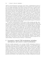
The simulation result of the controller is shown in Fig. 3, in which the
resultant torque curves are shown with control mode during one period (two
steps). In this figure, the control modes 1, 2, 3 and 4 correspond to swing
I, swing II, swing III and support, respectively. In Fig. 3, large torque is
-15
-10
-5
0
5
10
15
Torque [Nm]
1.41.21.00.80.60.40.20.0
Time [sec]
4
3
2
1
Control Mode
hip
knee
ankle
Control State
Fig. 3. State machine mode and torque during one period
observed at the end of the swing phase and the beginning of the support
phase. This torque might be caused by too large or too small torque applied
at the beginning of the swing phase. If the appropriate torque is applied in
swing I (at the beginning of the swing phase), this feedback torque might be

lessen and the more energy-efficient walking could be realized. In the next
section, the optimization of this torque is attempted by adding a learning
module.
3 Energy minimization by a learning module
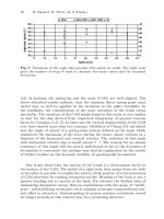
To realize the energy efficient walking, a learning module which searches
appropriate output torque in swing I is added to the controller described
in the previous section (Fig.4). Besides torque, the learning module searches
the appropriate value of control parameters which determine the end of the
duration of passive movement, T
swg2
. It is noted that these parameters are
not related to the PD controller which stabilizes walking. For the evaluation
of energy efficiency, we use the average of all the torque which is applied
during one walking period (two steps),
Eval =
1
T
step

T
step
0
3

i=1
τ
i
dt (10)
Using this performance function, the appropriate values of the parameters
are searched in the probabilistic ascent algorithm as follows.

160 M. Ogino, K. Hosoda, M. Asada
Learning Module
right leg
support
swing 1
swing 2
swing 3
Evaluation of Torque
Control
Parameters
(A,B,T
swg2)
State Machine Layer
left leg
swing 1
swing 2
swing 3
Fig. 4. Ballistic walking with learning module
1 if(Eval < Eval
min
)
2 A
min
= A
3 B
min
= B
4 T
swg2min
= T

swg2
5 A = A + random perturbation
6 B = B + random perturbation
7 T
swg2
= T
swg2
+ random perturbation
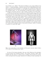
The simulation results are shown in Fig. 5. Figures 5 (a), (b) and (c) show
the time courses of the output torque applied to the hip and knee joints in
swing I,A,B,andthepassivetime,T
swg2
, and the average of total torque,
Eval, respectively. Even though the input torque changes variously, the PD
controller in swing III which keeps the posture at ground contact constant
realizes a stable walking.
1.2
0.8
0.4
0.0
Torque [Nm]
14012010080604020
Walking Step
Amin
A
Bmin
B
(a) torque
0.25
0.20

0.15
0.10
0.05
T
swg2
[sec]
14012010080604020
Walking Step
Tswg2min
Tswg
(b) T
swg2
12
10
8
6
4
Eval
14012010080604020
Walking Step
Eval_min
Eval
(c) average of total
torque
Fig. 5. Learning curve of control parameters and total torque
Comparing the first step with the 80th the average of total torque de-
creases (Fig. 5(c)), even though the output torque of the beginning of the
Learning Energy-Efficient Walking with Ballistic Walking 161
-15
-10

-5
0
5
10
15
Torque [Nm]
1.61.41.21.00.80.60.40.20.0
Time [sec]
4
3
2
1
Control Mode
ankle
knee
hip
Control State
Fig. 6. State machine mode and torque by a state machine controller with a learning
module
swing phase at the 80th step is almost the same as the first step (Fig. 5(a)),
whereas the passive time, T
swg2
, increases (Fig. 5(b)). The total torque of
walking, therefore, depends more on the passive time than the magnitude of
the feed forward torque that is given in the beginning of the swing phase.
Furthermore, in the final stage of learning, after the 120th step, the output
torque of the hip joint at the beginning in the swing phase becomes zero while
the torque of the knee joint increases. This result might be strange because
many researchers have applied torque to hip joint in swing phase. In this
stage, the large energy output appears among weak ones (Fig. 5(c)). This

may be because a robot walks on a wing and a prayer on the subtle balance
between dynamics and energy. Once the balance is lost, the PD controller
compensates stability with large torque.
Fig. 6 is the time-course of the torque around the 80th step. Comparing
the torque appeared in Fig. 6 with those in Fig. 3, the total torque are reduced
about 1/10 in the hip and knee joints, whereas the torque profile at the ankle
joint is almost the same.
4 Comparing with human data
In this section, we apply the proposed controller to the model that has the
same mass and length of links as human, and the torque and angle of each
link are compared with the observed data in human walking.
For parameters of human model, we use the same model as that of Ogihara
and Yamazaki [7], which is shown in Table 1. The control gains at hip and
knee joints are set as K
p
= 6000.0 [Nm/rad], K
v
= 300.0 [Nm sec/rad],
K
wp
= 6000.0 [Nm/rad] and K
wv
= 100.0 [Nm sec/rad]. The desired angles
at the end of the swing and support phases are the same as in Section 2.
The time course of angle and torque of the simulation results are shown
in Figs. 7 with human walking data (from [15]). The horizontal axis is nor-
malized by the walking period.
162 M. Ogino, K. Hosoda, M. Asada
Mass Length Inertia
[kg] [m] [kg m

2
]
HAT 46.48 0.542 3.359
Tigh 6.86 0.383 0.133
Shank 2.76 0.407 0.048
Foot 0.89 0.148 0.004
Table 1. Mass and length of human model links
-20
-10
0
10
20
Angle [deg]
100806040200
Walking Period [%]
4
3
2
1
Control State
(a) angle at hip joint
60
40
20
0
-20
Angle [deg]
100806040200
Walking Period [%]
4

3
2
1
Control State
(b) angle at knee joint
-20
-10
0
10
20
Angle [deg]
100806040200
Walking Period [%]
4
3
2
1
Control State
(c) angle at ankle
joint
80
60
40
20
0
-20
-40
-60
Torque [Nm]
100806040200

Walking Period [%]
4
3
2
1
Control State
Control State
Human
Simulation
(d) torque at hip joint
-100
-50
0
50
100
Torque [Nm]
100806040200
Walking Period [%]
4
3
2
1
Control State
(e) torque at knee
joint
120
80
40
0
Torque [Nm]

100806040200
Walking Period [%]
4
3
2
1
Control State
(f) torque at ankle
joint
Fig. 7. Comparing with human walking data
Human Simulation
Support : Swing [%:%] 60:40 60:40
Walking Rate [steps/sec] 1.9 1.3
Walking Speed [m/sec] 1.46 0.46
Walking Step [m] 0.76 0.36
Energy Consumption [cal/m kg] 0.78 0.36
Table 2. Characteristics of simulation and human walking
At the hip joint, while the time course of joint angle is almost same as
human, torque curve is quite different, especially in around 80% and 30%
walking periods in which strong effects of PD controllers appears (Fig. 7(b)).
At the knee joint, the pattern of the time course of joint angle roughly re-
sembles human data in shape except at around the end of the swing phase
Learning Energy-Efficient Walking with Ballistic Walking 163
and the beginning of the support phase, in which the knee joint of human
data becomes straighten but that of simulation data does not. Moreover, the
torque pattern is quite different from human data. At the ankle joint, it is
surprised that the torque pattern shares common traits with human data,
even though the ankle joint is modeled as simple spring joint. Fig. 7(f) shows
that, although the control state after the support phase is named ”swing I ”,
it works as double support phase. The rate of swing phase to support phase

is the same as human data (40:60).
Table 2 compares characteristics of walking in the simulation result with
that in human data ([12]). It shows that the simulation algorithm succeeds
in finding the parameters which enable the human model to walk with 45%
less energy consumption. But this walk may not necessarily mean the energy
efficient walking because the walking speed (and the walking rate) is much
slower than human walking. This may be because the proposed controller
uses the ankle joint only passively, and only the energy consumption is taken
into consideration in the evaluation function (eq. 10). Acquiring fast walking
is our future issue.
5 Discussion
Our controller has a state machine on each leg, which affects each other
by sensor signals. Even this simple controller enables a biped robot to walk
stably. There are two reasons. First, PD controllers at the end of the swing
phase ensure that a biped touches down on the ground with the same posture.
This prevents a swing leg from contacting with too shorter or too longer step
length because of inadequate forward torque given at the beginning of the
swing phase. But this stabilization does not always work well. It mainly
depends on the posture at ground contact. How this posture is determined is
the issue we should attack next.
The second reason for stable walking is that the controller has some com-
mon features to CPG (Central Pattern Generator). In the CPG model, the
activities of neurons are affected by sensor signals (or environment), and as
a result global entrainment between a neural system and the environment
takes place [14]. Our proposed controller doesn’t have a walking period ex-
plicitly. The period of the controller is strongly affected by the information
from touch sensors, which determine the state transition of a state machine
in each leg. It can be said that our controller has some properties like global
entrainment between the state machine controller and the environment.
Walking mode realized in this paper is much slower than human walking

as shown in Table 2. We suppose that the reason of this slow walking owes
to the passive use of the ankle joint. To realize fast walking, it is necessary
to shorten the walking period and to make the step length longer. They are
closely related to the ankle joint setting because the speed of falling forward
of the support leg is largely affected by the stiffness of the ankle joint, and the
164 M. Ogino, K. Hosoda, M. Asada
step length can be longer if the support leg rotates around the toe. Controlling
the walking speed is another issue to be attacked.
Acknowledgments
This study was performed through the Advanced and Innovational Research
program in Life Sciences from the Ministry of Education, Culture, Sports,
Science and Technology, the Japanese Government.
References
1. Asano, F. Yamakita, M. and Furuta, K., 2000, “Virtual passive dynamic walk-
ing and energy-based control laws”, Proceedings of the 2000 IEEE/RSJ Int.
Conf. on Intelligent Robots and Systems, pp. 1149-1154.
2. Garcia, M. Chatterjee, A. Ruina, A. and Coleman, M., 1998, “The simplest
walking model: stability, complexity, and scaling”, J. Biomechanical Engineer-
ing, Vol. 120, pp. 281-288.
3. Goswami, A. Thuilot, B. and Espiau, B., 1998, “A Study of the Passive Gait of
a Compass-Like Biped Robot: symmetry and Chaos”, Int. J. Robotics Research,
Vol. 17, No. 12, pp.1282-1301.
4. Van der Linde, R, Q., 2000, “Actively controlled ballistic walking”, Proceed-
ings of the IASTED Int. Conf. Robotics and Applications 2000, August 14-16,
Honolulu, Hawaii, USA.
5. McGeer, T., 1990, “Passive walking with knees”, 1990 IEEE Int. Conf. on
Robotics and Automation, 3, Cincinnati, pp.1640-1645.
6. Mochon, S. and McMahon, T.A., 1980, “Ballistic walking”, J. Biomech., 13,
pp. 49-57.
7. Ogihara, N. and Yamazaki, N., 2001, “Generation of human bipedal locomotion

by a bio-mimetic neuro-musculo-skeletal model”, Biol. Cybern., 84, pp. 1-11.
8. Ogino, M. Hosoda, K. and M, Asada., 2002, “Acquiring passive dynamic walk-
ing based on ballistic walking”, 5th Int. Conf. on Climbing and Walking Robots,
pp.139-146.
9. Ono, K. Takahashi, R. Imadu, A. and Shimada, T., 2000, “Self-excitation con-
trol for biped walking mechanism”, Proceedings of the 2000 IEEE/RSJ Int.
Conf. on Intelligent Robots and Systems, pp. 1149-1154.
10. Osuka, K. and Kirihara, K., 2000, “Development and control of new legged
robot quartet III - from active walking to passive walking-”, Proceedings of the
2000 IEEE/RSJ Int. Conf. on Intelligent Robots and Systems, pp. 991-995.
11. Pratt, J., 2000, “Exploiting Inherent Robustness and Natural Dynamics in the
Control of Bipedal Walking Robots”, Doctor thesis, MIT, June.
12. Shumway-Cook, A. Woollacott, M., 1995, “Motor Control : Theory and Prac-
tical Applications”, Williams and Wilkins.
13. Sugimoto, Y. and Osuka, K., 2002: “Walking control of quasi-passive-dynamic-
walking robot ’Quartet III’ based on delayed feedback control”, Proceedings of
the Fifth Int. Conf. on Climbing and Walking Robots, pp. 123-130.
14. Taga, G., 1995, “A model of the neuro-musculo-skeletal system for human lo-
comotion: I. Emergence of basic gait”, Biol. Cybern., 73, pp. 97-111.
15. Winter, DA., 1984, “Kinematic and kinetic patterns of human gait; variability
and compensating effects”, Human Movement Science, 3, pp. 51-76.
Motion Generation and Control of Quasi
Passsive Dynamic Walking Based on the
Concept of Delayed Feedback Control
Yasuhiro Sugimoto and Koichi Osuka
Dept. of Systems Science, Graduate School of Informatics, Kyoto University, Uji,
Kyoto, 611-0011, JAPAN
Abstract. Recently, Passive-Dynamic-Walking (PDW) has been noticed in the
research of biped walking robots. In this paper, focusing on the entrainment phe-
nomena which is the one of character of PDW, we provide a new control method of

Quasi-Passive-Dynamic-Walking. Concretely, at first, for the sake of the continuous
walking of robot and taking place of the entrainment phenomenon, we adopt a kind
of PD control which gains are regulated by the state of the contact phase of swing
leg. And, considering the making use of the concept of DFC, we use (k-1)-th trajec-
tory of the walking robot as the reference trajectory of the k-th step. As a result, it
can be expected that the robot itself generates the optimum stable trajectory and
the walking is stabilized by using this trajectory.
1 Introduction
Recently a lot of researches of humanoid robots or biped locomotion have
been carried out. ASIMO(HONDA) and HRP-series(AIST) are very famous
examples. In such researches of walking robots, recently, Passive Dynamic
Walking(PDW) which was studied by McGeer[1] at first, has been noticed.
As the features of this motion, the following are raised: This walking is very
smooth and similar to human’s walking. Secondly, it can be realized only
by the dynamics of robot without any input torques if the robot walks on
smooth slope. Moreover, by using the effect of gravitational field skillfully,
the robot walks with high energy efficiency. From these features, the various
studies of applications of PDW have been made expecting a realization of a
high-efficient and smooth walking of robot [2][3][4][5][6].
Especially, in the application of PDW, some control methods of Quasi-
Passive-Dynamic-Walking(Quasi-PDW) have been proposed [4][5][6]. Quasi-
PDW means that the robot usually does PDW without any torque inputs,
and just only when the walking begins or disturbances come in, the actuators
of the robot are used for stabilization of walking. As one of this control
method, focusing the contact phase of the swing leg with the ground (we
call it’s state Impact point), we proposed a control method which based on
Delayed Feedback Control(DFC) [5][6]. This control method is very simple
and does not require making any reference trajectory. But, it can not stabilize
the walking without a proper set of initial conditions. (especially it requires
166 Yasuhiro Sugimoto, Koichi Osuka

proper initial velocities) And since it focuses just only on impact point, the
performance of stabilization is relatively small.
Then, refering to the one of the control method of Quasi-PDW[4], we
consider both following two: one is to make use of the concept of the DFC
and the second one is to provide some reference trajectory for continuous
walking. From the above, in this paper, we will propose a new control method
in which (k-1)-th step’s trajectory of the walking robot are used as k-th
reference trajectory and the PD gains in this control low are regulated in each
steps depending on the state of the impact point. By doing so, it is expected
that the robot walks continuously and the entrainment phenomena of PDW
will occur, and then, its walking will converge to the stable trajectory. This
trajectory is equivalent to the trajectory which the robot in PDW generates.
This means that the robot walking finally becomes to be stabilized by using
PDW trajectory which is made by the robot itself.
2 Model of the walking robot
A model of the biped robot which we consider is shown in Fig.1.
Fig. 1. Compass model of Walking robot
Let the support leg angle be θ
p
, the swing (non-supported) leg angle be
θ
w
, a slope angle be parameter α, and a torque vector which is supplied to
the support leg and the swing leg be τ(t)=[τ
p
,τ
w
]
T
.Andβ is the support

leg angle at the collision of the swing leg with the ground. Then, the dynamic
equation of the robot can be derived using the well known Euler-Lagrange
approach:
M(θ)
¨
θ + N(θ,
˙
θ)
˙
θ + g(θ, α)=τ(t), (1)
where M(θ) is the inertia matrix, N (θ,
˙
θ)
˙
θ is the centrifugal and Colioris term,
and g(θ, α) is the gravity term. See [4] or [6] in detail. If we assume that a
transition of the support leg and the swing leg occurs instantaneously and
Motion Generation and Control of Quasi Passsive Dynamic Walking 167
the impact of the swing leg with the ground is inelastic and occurs without
sliding, the equation of transition at the collision can be derived by using the
conditions of conservation of angular momentum:
P
b
(β)
˙
θ
−
= P
a
(β)

˙
θ
+
, (2)
where
˙
θ
−
,
˙
θ
+
are the pre-impact and the post-impact angular velocities re-
spectively. The details of P
b
(β), P
a
(β) are provided in [4] or [6].
And we difine an vector p as:
p(k)=(β
k
,
˙
θ
−
p,k
,
˙
θ
−

w,k
)
T
, (3)
where β
k
is β at the k-th collision,
˙
θ
−
p,k
and
˙
θ
−
w,k
are the k-th pre-impact
angular velocities of the support leg and the swing leg respectively. And we
call this p as Impact point.
3 Stability of passive dynamic walking
If the input torques are assumed to be constant over each k-th step and some
assumptions will be hold, it can be stated that the discrete dynamic system of
impact point: p(k +1) = P(p(k),τ(k)) can be well defined and the stability of
the equilibrium point of this system is equivalent to the stability of PDW [5].
Here, expanding this statement, we show that the stability of the equilibrium
point of this system is equivalent to the stability of PDW even if the input
torques are not constant but continue and differentiable between each k-th
step.
Theorem 1 Let the input torques τ(t) be continue and differentiable be-
tween each k-th step. Then, with regard to impact point p(k) and input

torques τ(t), a following map P
cl
p(k +1)=P
cl
(p(k),τ)(4)
can be defined. And, p
∗
is a stable equilibrium point of this map Eq.(4) with
τ(t)=0for T
p
(k −1) ≤ t
∀
<T
p
(k), if and only if, the continuous trajectory
of the motion of the robot that passes through p
∗
is stable in the sense of
Lyapunov, where T
p
(k) is a time when the k-th impact occurs.
Proof Basically, it can be proved by similar way of the proof of lemma 1
and 2 in [5]. At first, let the set of the states of the robot just before impact
be S, then the target system of the robot can be denoted as follows:
Σ :

˙x(t)=f
cl
(x(t)) (x
−

(t) ∈S)
x
+
(t)=∆(x
−
(t)) (x
−
(t) ∈S),
(5)
where,
x(t):=(θ
p
,θ
w
,
˙
θ
p
,
˙
θ
w
)
T
,f
cl
:= f(x(t)) + g(x(t))τ(t),
f(x(t)) =

(

˙
θ
p
,
˙
θ
w
)
T
−M
−1
(θ)(N(θ,
˙
θ)
˙
θ + g(θ, α))

,g(x(t)) =

0
M
−1
(θ)

.
168 Yasuhiro Sugimoto, Koichi Osuka
Because of the condition of τ(t), it can be said that f
cl
(t) can have a unique
solution which depends continuously on the initial condition between the

each k-th step, and then, the map P
cl,x
(x, τ) can be well-defined [7]. This
map means that the state just before the k-th collision x
−
k
is mapped to the
state just before the (k+1)-th collision x
−
k+1
when input torques τ are used.
Then, using the following matrixes:
E =
⎛
⎜
⎝
100
−100
010
001
⎞
⎟
⎠
,F =

1000
0010
0001

,

wecandefinedamapP
cl
(p(k),τ) as follows:
p(k +1)=FP
cl,x
(Ep(k),τ(k)): = P
cl
(p(k),τ). (6)
Secondly, because the existence of the map P
cl,x
(x, τ) can be shown, using the
same way of proof of lemma 2 in [5], we can say that p
∗
is a stable equilibrium
point of the system: p(k +1)=P
cl
(p(k),τ) with τ(t)=0for T
p
(k − 1) ≤
t
∀
<T
p
(k), if and only if, the continuous trajectory of the robot that passes
through p
∗
is stable in the sense of Lyapunov.
From this theorem, it can be said that even if the input torques are not
constant but continue and differentiable between each k-th step, the stability
of impact point p(k) on the discrete dynamical system is greatly related to

the stability of PDW.
4 DFC-based control method
To propose a new control method of Quasi-Passive-Dynamic-Walking, we
particularly consider the following two key ideas. The first one is making use
of the concept of DFC so as not to design the reference trajectory which the
robot in PDW generates correctly. The second one is providing roughly de-
signed reference trajectory and stabilizing the walking by using this reference
trajectory so as to be possible to start its walking without a proper initial
condition or to continuous walking even if some disturbances come in.
To construct new controller with the above ideas, in this paper, we focus
on the entrainment phenomena which is one of the properties of PDW. The
entrainment phenomena of PDW means that even if the robot starts walking
with different initial conditions, its walking converges to a specific trajectory
which is agree with the trajectory of PDW. However, the states of robot which
can cause the entrainment phenomena will exist in narrow region because the
initial conditions which can cause PDW exist in very narrow region and PDW
is very sensitive to disturbance. So, it seems that it is difficult to stabilize
Quasi-Passive-Dynamic-Walking only by using the entrainment phenomena.
Then, we construct a new control method which has the next two proper-
ties, that is, “generation of PDW using the entrainment phenomena and the
Motion Generation and Control of Quasi Passsive Dynamic Walking 169
concept of DFC so as to be needless of correctly design of the reference tra-
jectory of PDW” and “stabilization the walking for the sake of its continuous
walking and taking place of the entrainment phenomena”.
4.1 Our previous control method of quasi-PDW
Discrete-DFC based control method As an example of the control
method of Quasi-PDW, the discrete-DFC based control method [5] or [6] can
be given. This control method is that, since it can be proved that the stability
of PDW is equivalent to the stability of the equilibrium impact point on the
discrete dynamical system:

p(k +1)=P(p(k),τ), (7)
Quasi-Passive-Dynamic-Walking can be stabilized by using the input torques
τ(k) which stabilize p(k) of the system Eq.(7):
τ(k)=K(y(k) − y(k − 1)) = K

P
p
(k) −P
p
(k − 1)
P
w
(k) −P
w
(k − 1)

, (8)
where P
p
(k),P
w
(k) are the kinetic energy of the support and swing leg at
impact point respectively. From Eq.(8), we can see that this control method
is very simple and does not need any information of the equilibrium point p
∗
of Eq.(7), that is, it can stabilize Quasi-PDW without making any reference
trajectory. However, focusing only on impact point, the performance of this
control method is relatively not so good. So, this can not stabilize the walk-
ing when big disturbances come in. Furthermore, this can not stabilize the
walking without proper initial conditions especially initial velocities of the

legs.
Weekly guidance control method On the contrary, as one of the con-
trol method which utilizes the entrainment phenomena, Osuka and Saruta
proposed the following control method [4] (we call it “weekly guidance control
method”):
τ = K
f
(δ(k))[M(θ)s + N (θ)
˙
θ
2
+ g(θ,α)], (9)
δ(k)=β(k) −β(k − 1),
s =
¨
θ
d
+ K
v
(
˙
θ
d
−
˙
θ)+K
p
(θ
d
− θ),

where, K
f
(x) is defined by
K
f
(x)=

1 x≥γ
(−cos(
xπ
γ
)+1)/2 x≤γ,
(10)
and an example of K
f
(x) is shown in Fig.2.
As the features of this control method, the following can be given: |β
k
−
β
k−1
| is adopted as an evaluate function of the stability of walking and it is
170 Yasuhiro Sugimoto, Koichi Osuka
Fig. 2. Example of function K
f
at γ =1.0
used as the weight of trajectory tracking controller. According to the features,
even if there is an error between the reference trajectory r
d
=[θ

d
,
˙
θ
d
] used
in this control method and the trajectory r
id
=[θ
id
,
˙
θ
id
] which the robot
in PDW generates, the trajectory of robot converges to r
id
and |β
k
− β
k−1
|
becomes small gradually during the robot walks continuously, owing to the
entrainment phenomena. And finally, |β
k
−β
k−1
| becomes zero and then the
robot becomes to do PDW. Therefore, it can be expected that Quasi-PDW,
will be realized by using this control method.

However, we think that there are the following problems in this control
method (9).
• In case that the robot’s walking is disordered by some disturbances
after its walking converges to r
id
, that is, after robot come to do PDW,
is it unreasonable to make the walking to converge to PDW using the r
d
once again ? Since the ideal trajectory r
id
will be made already by robot
itself, are there some method of making use of r
id
for stabilization of its
walking ?
• How on earth do we make the reference trajectory r
d
?
• From Section 3, is it better to use the data of impact point p(k)than
β
k
when the stability of walking is evaluated ?
Especially, with regard to r
d
, even if there would be some differences between
r
d
and r
id
, we could expect the walking would converge to r

id
owing to the
entrainment phenomena. But, it is desired that the difference between r
d
and
r
id
is as small as possible to improve the efficiency of this control method.
Therefore, it is needed to make a sufficient proper reference trajectory r
d
in
advance, and then, it can not be said any more that this control method fully
makes use of the entrainment phenomena of PDW.
4.2 The propose control method
From 4.1, 4.1 and the consequence of Section 3 which means that the impact
point p(k) is greatly related to the stability of robot’s walking, we propose
the following control method.
Motion Generation and Control of Quasi Passsive Dynamic Walking 171
Updating reference trajectory control method based on DFC
τ
k
= K
f
(δ
k
)[K
v
(
˙
θ

k−1
−
˙
θ
k
)+K
p
(θ
k−1
− θ
k
)] (11)
δ
k
= ||p(k) − p(k − 1)||
φ
,
where θ
k
is k-th step’s θ =(θ
p
,θ
w
)
T
, K
f
(·) is defined by Eq.(10), φ is a
constant matrix φ ∈R
3×3

and ||·||
M
is a norm defined by ||x||
M
=
√
x
T
Mx
and a constant matrix M ∈R
m×n
.
As one of the features of this control method(11), the following can be
given: at first, it evaluates the stability of walking by using the data of impact
point p(k)andp(k − 1). And secondly, it realizes tracking control not with
r
d
which is made in advance but with r
k−1
which is the (k-1)-th trajectory
of robot. As a result, the reference trajectory is updated in each steps.
Since the walking is stabilized by PD-control whose gains are regulated
depending on the stability of walking, it can be said that this proposed control
method (11) satisfies the specification which is “stabilization of the walking
for the sake of its continuous walking and taking place of the entrainment
phenomena”.
And, since updating the reference trajectory using the (k-1)-th step trajec-
tory in each steps is equivalent to doing continuous-DFC and the entrainment
phenomena will cause because walking will continue, we can expect that its
walking will converge to r

id
without making correctly design of the trajec-
tory r
id
during the robot walks continuously. Therefore, the proposed control
method can satisfy the secondary specification which is “to generate of PDW
using the entrainment phenomena and the concept of DFC so as to be need-
less of correctly design of the reference trajectory of PDW”. Moreover, if once
the walking of robot converges to PDW, it holds true that r
k
= r
k−1
= r
id
.
So, it is also the advantage of this control method that it can use r
id
as the
reference trajectory after the convergence to PDW.
Furthermore, with regard to initial reference trajectory r
0
, since it can ex-
pected that the robot itself makes the ideal trajectory r
id
during the walking,
it is enough to design r
0
roughly with which walking can be occur without
falling down.
Remark In case of using the proposed method Eq.(11) with a real robot,

it is more reasonable that we obtain r
id−sim
by some simulation using the
proposed method with an roughly designed r
0
at first, then we use this r
id−sim
as r
0
when we actually apply the proposed method to the real robot.
5 Computer simulation
In this section, we investigate the validity of the proposed control method (11)
by several simulations. We use same physical parameters of robot as Quartet
III [4]. The initial conditions of the robot are set as θ
0
(0) = [−0.34, 0.34, 0, 0]
T
and
172 Yasuhiro Sugimoto, Koichi Osuka
K
p
=

30 0
030

,K
v
=


25 0
025

,φ=

50 0
00.10
000.1

,γ=1.0.
The initial reference trajectory r
0
(t) is set as,
θ
p,0
(t)=2.2667t
2
+0.79333t − 0.34000,
˙
θ
p,0
(t)=4.4894t +0.79333,
θ
w,0
(t)=8.4524t
2
− 5.0810t −0.34000,
˙
θ
w,0

(t)=16.905t − 5.0810.
These are obtained as following. At first, θ
p
(t)andθ
w
(t) are given as quadratic
equations which pass [(0,-0.34),(0.25,0),(0.4,0.34)] and [(0,0.34),(0.3,-0.4),(0.4,-
0.34)] respectively. Then,
˙
θ
p
(t)and
˙
θ
w
(t) are obtained by differentiating θ
p
(t)
and θ
w
(t) respectively. Furthermore, since it can be that k-th step’s walking
period is bigger than (k-1)-th step’s walking period, we use a 7th polynomial
which is approximated to (k-1)-th step’s trajectory as k-th step’s reference
trajectory.
Simulation results are shown in Fig.3-Fig.5. Fig.3 shows the support leg
angle and swing leg angle θ
p
(t)andθ
w
(t). Fig.4 shows the input torques

τ(t), where the solid line means the support leg and the dotted line means
the swing leg respectively. Fig.5 shows the 1,2,3,7 and 24th step’s reference
trajectory respectively. To compare with our previous control method, the
simulation results with weekly guidance control method Eq.(9) in which the
same r
0
is used as the reference trajectory, are shown in Fig.6 and 7.
0 1 2 3 4 5 6 7 8 9 10
- 0.5
0
0.5
time[sec]
θ
p
, θ
w
[rad]
support leg
swing leg
Fig. 3. Trajectory of θ
p
,θ
w
by Eq.(11)
0 1 2 3 4 5 6 7 8 9 10
-20
-15
-10
- 5
0

5
10
15
20
time[sec]
torque [Nm]
support leg
swing leg
Fig. 4. Input torque by Eq.(11)
From these figures, though the robot’s walking is not uniformly and the
input torques are needed to continue walking at the beginning of walking,
the input torques τ and K
f
are decreasing gradually during some steps. And
finally, r
k
becomes equivalent to r
k−1
and the robot becomes to walk via
PDW. On the contrary, the robot’s waking with the weekly guidance control
can not converge to PDW though the robot can continue walking. This is
because it does not use the proper reference trajectory r
d
.So,wecansay
that the proposed control method Eq.(11) works well.
Secondly, we investigate the robustness of the proposed control method
against disturbance. Simulation results in which the slope angle α is set as
Motion Generation and Control of Quasi Passsive Dynamic Walking 173
0 0.1 0.2 0.3 0.4
- 0.5

- 0.4
- 0.3
- 0.2
- 0.1
0
0.1
0.2
0.3
0.4
0.5
time[sec]
θ
p
[rad]
step 1
step 2
step 7
step 10
step 24
Fig. 5. Reference trajectory of θ
p
0 1 2 3 4 5 6 7 8 9 10
- 0.5
0
0.5
time[sec]
θ
p
, θ
w

[rad]
support leg
swing leg
Fig. 6. Trajectory of θ
p
,θ
w
by Eq.(9)
0 1 2 3 4 5 6 7 8 9 10
- 0.5
0
0.5
time[sec]
θ
p
, θ
w
[rad]
support leg
swing leg
Fig. 7. Input torque by Eq.(9)
6[deg] (nominal value of α is 3[deg]) between 5[sec]and6[sec], are shown
in Fig.8 and 9. To compare with our previous control methods, simulation
results when Eq.(8) and Eq.(9) are used are also shown in the same figures.
Here, there is a problem how we set the reference trajectory r
d
in Eq.(9).
In this simulation, for easily convergence to PDW, we make the reference
trajectory which is very close to the trajectory of PDW but is not agree
perfectly and use it.

0 1 2 3 4 5 6 7 8 9 10
- 0.5
0
0.5
time[sec]
θ
p
, θ
w
[rad]
proposed method Eq.(10)
discret DFC method Eq.(7)
weekly guidance method Eq.(8)
Fig. 8. Trajectory of θ
p
,θ
w
0 1 2 3 4 5 6 7 8 9 10
-20
-15
-10
- 5
0
5
10
15
20
time[sec]
torque [Nm]
propose method Eq.(10)

discreteDFC method Eq.(7)
w eekly guidance methol Eq.(8)
Fig. 9. Input torque
174 Yasuhiro Sugimoto, Koichi Osuka
From these figures, we can see that the robot with the discrete-DFC based
control Eq.(8) can not continue walking after the disturbance is added, and
the robot with the weekly guidance control Eq. (9) can not converge to PDW
again. On the contrary, the robot with the proposed method Eq.(11) can
walk down continually after the disturbance is added and becomes to walk
via PDW again. So we can say that the proposed method works well.
6 Conclusion and future work
In this paper, making use of the concept of DFC and the entrainment phe-
nomena of PDW, we proposed a new control method of Quasi-PDW. Con-
cretely, the proposed method uses (k-1)-th step’s trajectory of the walking
as the reference trajectory of the k-th step and regulates the gain according
to impact Point. And the effectiveness of the proposed control method was
shown through several simulations.
As a problem yet to be solved in the future is to prove the effectiveness of
the proposed control method and obtain the systematic derivation methods
of K
p
,K
v
and φ in Eq.(11). Furthermore, we should carry out experiments
with a real robot.
References
1. T.McGeer: “Passive Dynamic Walking”, Int.J.of Rob.Res., Vol.9, No.2, 1990
2. A. Goswami, B. Thuilot and B. Espiau: “A Study of the Passive Gait of
a Compass-Like Biped Robot: Sysmmetry and Chaos”,Int. J.of Rob. Res.
pp.1282–1301,2000

3. F. Asano, M. Yamakita, N. Kamamichi, Z. LUO, “A Novel Gait Generation
for Biped Walking Robots Based on Mechanical Energy Constraint”, Proc. of
the IEEE/RSJ Int. Conf. on Intellignet Robots and Systems(IROS), pp.2637–
2644, 2002
4. K.Osuka,Y.Saruta: “Gait Control of Legged Robot Quartet III via Passive
Walking”, Proc. of the 8 th Symposium on Control Technology8th, pp.355–
360,2000 ( in Japanese)
5. Y. Sugimoto, K. Osuka, “Stabilization of semi passive dynamic walking based
on delayed feedback control”, Proc. of the 7 th Robotics Symposia, pp89–94,
2002 (in Japanese)
6. Y. Sugimoto, K. Osuka, “Walking Control of Quasi-Passive-Dynamic-Walking
Robot “Quartet III” based on Delayed Feedback Control”, Proc.ofthe5th
Int. Conf. on Climbing and Walking Robots(CLAWAR), pp.123–130, 2002
7. J. W. Grizzle, F. Plestan and G. Abba: “Poincare’s Method for Systems with
Impulse Effects: Application to Mechanical Biped Locomotion”, Proc.ofthe
38th Conference on Decision & Control, pp. 3869–3876,1999
8. K.Pyragas,“Continuous control of chaos by selfcontrolling feedback”,
Phys.Lett.A,vol 170,pp.421–428,1992
Part 5
Neuro-Mechanics
& CPG and/or Reflexes
Gait Transition from Swimming to Walking:
Investigation of Salamander Locomotion
Control Using Nonlinear Oscillators
Auke Jan Ijspeert
1
and Jean-Marie Cabelguen
2
1
Swiss Federal Institute of Technology, CH-1015 Lausanne, Switzerland

2
Inserm EPI9914, Inst. Magendie 1 rue C. St-Sa¨ens, F-33077 Bordeaux, France
Abstract. This article presents a model of the salamander’s locomotion controller
based on nonlinear oscillators. Using numerical simulations of both the controller
and of the body, we investigated different systems of coupled oscillators that can
produce the typical swimming and walking gaits of the salamander. Since the exact
organization of the salamander’s locomotor circuits is currently unknown, we used
the numerical simulations to investigate which type of coupled-oscillator configu-
rations could best reproduce some key aspects of salamander locomotion. We were
in particular interested in (1) the ability of the controller to produce a traveling
wave along the body for swimming and a standing wave for walking, and (2) the
role of sensory feedback in shaping the patterns. Results show that configurations
which combine global couplings from limb oscillators to body oscillators, as well
as inter-limb couplings between fore- and hind-limbs come closest to salamander
locomotion data. It is also demonstrated that sensory feedback could potentially
play a significant role in the generation of standing waves during walking.
1 Introduction
The salamander, a tetrapod capable of both swimming and walking, offers a
remarkable opportunity to investigate vertebrate locomotion. It represents,
among vertebrates, a key element in the evolution from aquatic to terrestrial
habitats.
This article investigates the mechanisms underlying locomotion and gait
transition in the salamander. We develop computational models of the spinal
circuits controlling the axial and limb musculature, and investigate how these
circuits are coupled to generate, and switch between, the aquatic and terres-
trial gaits. In previous work, one of us developed neural network models of
the salamander’s locomotor circuit based on the hypothesis that the circuit
is constructed from a lamprey-like central pattern generator (CPG) extended
by two limb CPGs [2]. In that work, a genetic algorithm was used to instan-
tiate synaptic weights in the models such as to optimize the ability of the

CPG to generate salamander-like swimming and walking patterns. Here, we
develop models based on coupled nonlinear oscillators, and extend that work
by systematically investigating different types of couplings between the oscil-
lators capable of producing the patterns of activity observed in salamander
178 Auke Jan Ijspeert and Jean-Marie Cabelguen
Neck
Trunk
Tail
Forelimb
CPG
CPG
Body
Hindlimb
CPG
1
5
10
15
20
25
30
35
40
Fig. 1. Left: Schematic dorsal view of the salamander’s body. Right: Patterns of
EMG activity recorded from the axial musculature during swimming (top) and
walking (bottom), adapted from Delvolv´e et al. 1997.
locomotion. The use of nonlinear oscillators instead of neural network oscilla-
tors allows us to reduce the number of state variables and parameters in the
models, and to focus on a systematic study of the inter-oscillator couplings.
We address the following questions: (1) how are body and limb CPGs

coupled to produce traveling waves of lateral displacement of the body during
swimming and standing waves during walking? (2) how is sensory feedback
integrated into the CPGs? (3) does sensory feedback play a major role in
the transition from traveling waves to standing waves? (4) to what extent
is the inter-limb coordination between fore and hind limbs due to inter-limb
coupling and/or the coupling with the body CPG? Clearly most of these
questions are relevant to tetrapods in general.
2 Neural control of salamander locomotion
The salamander uses an anguiliform swimming gait very similar to the lam-
prey. The swimming is based on axial undulations in which rostrocaudal
waves with a piece-wise constant wavelength are propagated along the whole
body with limbs folded backwards (Figure 1, right). As in the lamprey, the
average wavelength usually corresponds to the length of the body (i.e. the
body produces one complete wave) and does not vary with the frequency of
oscillation [3]. On ground, the salamander switches to a stepping gait, with
the body making S-shaped standing waves with nodes at the girdles [3]. The
stepping gait has the phase relation of a trot, in which laterally opposed
limbs are out of phase, while diagonally opposed limbs are in phase. The
limbs are coordinated with the bending of the body such as to increase the
stride length in this sprawling gait. EMG recordings [3] have confirmed the
bimodal nature of salamander locomotion, with axial traveling waves along
Gait Transition from Swimming to Walking 179
Retractor
Joints
Tail
Muscles
4
5
6
7

8
9
10
11
12
ProtractorRigid linksFoot contact
14
15
13
16
Trunk
Neck
1
2
3
−2 −1.5 −1 −0.5 0 0.5 1 1.5
−1.5
−1
−0.5
0
0.5
1
1.5
X
V
Fig. 2. Left: Mechanical model of the salamander’s body. The two-dimensional
body is made of 16 rigid links connected by one-degree-of-freedom joints. Each
joint is actuated by a pair of antagonist muscles simulated as spring and dampers.
Right: Limit cycle behavior of the nonlinear oscillator, time evolution with different
random initial conditions.

the body for swimming, and mainly standing waves coordinated with the
limbs for walking (Figure 1).
The CPG underlying axial motion —the body CPG— is located all along
the spinal cord. Similarly to the lamprey [1], it spontaneously propagates
traveling waves corresponding to fictive swimming when induced by NMDA
excitatory baths in isolated spinal cord preparations [4]. Small isolated parts
of 2 to 3 segments can be made to oscillate suggesting that rhythmogenesis
is similarly distributed in salamander as in the lamprey. The neural centers
for the limb movements are located within the cervical segments C1 to C5
(Figure 1 left) for the forelimbs and within the thoracic segments 14 to 18
for the hindlimbs [5–7]. These regions can be decomposed into left and right
neural centers which independently coordinate each limb [5,7].
3 Mechanical simulation
The two-dimensional mechanical simulation of the salamander is an exten-
sion of Ekeberg’s simulation of the lamprey [8]. The 25 cm long body is made
of twelve rigid links representing the neck, trunk and tail, and four links
representing the limbs (Figure 2). The links are connected by one-degree-
of-freedom joints, and the torques on each joint are determined by pairs
of antagonist muscles simulated as springs and dampers. The signals sent by
the motoneurons contract muscles by modifying (increasing) their spring con-
stant. The accelerations of the links are due to four types of forces: the torques
due to the muscles, inner forces linked with the mechanical constraints due
to the joints, contact forces between body and limbs, and the forces due
to the environment (friction on ground, and inertial hydrodynamic forces in
water). The dynamics equations underlying the simulation are described in
more detail in [2].