Advances in Robot Kinematics - Jadran Lenarcic and Bernard Roth (Eds) Part 5 pps
Bạn đang xem bản rút gọn của tài liệu. Xem và tải ngay bản đầy đủ của tài liệu tại đây (1.44 MB, 30 trang )
can only As Hunt
stated in Chapter 4 of his book (Hunt, 1978):
Yet neither Kempe nor anyone else since has established a method
for isolating the best, or the simplest, linkage for tracing a particular
curve.
In the history all feasible linkages with a small number of links for
algebraic curves generation were invented by somegreatmasters using
their geometrical intuitions (Please see the Appendix for details). Nev-
ertheless geometrical intuitions are di
may not guarantee all solutions for a synthesis problem be found. The
above investigation raises a question: Are there any undiscovered 6-bar
linkages for straight-line generation? This paper proposes a numerical
approach to attack the problem. Notethatitispossibletoextendthe
approach for nding spatial 6R single loop overconstrained mechanisms
(see remarks at the end of Section 2.2).
2.
Figure 1. Six arrangements of 6-bar linkages for a path generation, with the asterisk
denoting the position of coupler-point
Figure 1 illustrates 6 possible arrangements of 6-bar linkages for straight-
line generation. As can be seen from Fig. 4 that the existing straight-line
6-bar linkages are either Watt-I1 linkages or Stephenson-I linkages. In-
deed based on the principle of inversion and Robert’s cognate theorem,
we can conclude that Stephenson-II2 linkages and Stephenson-III link-
ages cannot generate a straight-line. Other arrangements should be
1
This is still an open problem. Smith, 1998 tried to prove it but failed.
2
According to (Artobolevskii, 1964), Alekseyev, 1939 discovered the dimensional relationships
of the generalized linkage on 1939, but the authors are not able to find Alekseyev’s proof,
while the short proof given in Artobolevskii’s book is indeed invalid.
Z. Luo and J.S. Dai114
Searching for 6-bar Straight-line Linkages
.
find feasible linkages with a large number of links .
fficult to be duplicated, and they
to the derivation of coupler-curve equations of general planar linkages
(see Primrose et al., 1967, Almadi, 1996, and Wampler, 1999). However
it is important to develop problem-speci
analysis (Dukkipati, 2001, Karger, 1998) or numerical analysis (Luo and
Dai, 2005).
2.1 Synthesize Stephenson-I Linkages for
Figure 2. Two representations for synthesizing Stephenson-I linkages. (a) is Alek-
seyev’s representation (see Artobolevskii, 1964), and (b) is a new representation
In Alekseyev’s representation, suppose a coupler-curve equation in
(x
Q
,y
Q
) is obtained, the coupler curve is a straight line if and only if
there exist (x
0
,θ) which satisfy y
Q
≡ tan θ (x
Q
− x
0
). However since
tan θ can vary from zerotoin nity,(x
Q
,y
Q
) should be parameterized.
In our representation, we assume the straight-line is along the x-axis,
thus y
Q
≡ 0. We further specify x
A
= 0. As can be seen, there are 10
structural parameters (a, b, c, e, f, g, h, y
A
,x
D
,y
D
). Alternatively we can
use (a, b, c, d, e, f, g, h, y
A
,θ
0
). Refer to Fig. 2(b), we obtain the following
three loop-closure equations:
a cos θ
1
+ b cos θ
2
− c cos θ
3
= x
D
− x
A
a sin θ
1
+ b sin θ
2
− c sin θ
3
= y
D
− y
A
(1)
(a + e)cosθ
1
+ f cos θ
4
= x
Q
− x
A
(a + e)sinθ
1
+ f sin θ
4
= y
Q
− y
A
(2)
(c + h)cosθ
3
+ g cos θ
5
= x
Q
− x
D
(c + h)sinθ
3
+ g sin θ
5
= y
Q
− y
D
(3)
Using classic resultant methods, it is not di
i
1, ,5) and a 16
th
degree bivariate polynomial in (x
Q
,y
Q
) is obtained.
Searching for Undiscovered Planar Straight-line Linkages
115
examined individually. Synthesizing straight-line linkages is closely related
a Straight-line Motion
.
fic methods based on symbolic
fficult to eliminate θ (i =
Since y
Q
≡ 0, we obtain a univariate polynomial in x
Q
. Denote it as:
P
s1
=
16
i=0
a
i
x
i
Q
=0 (4)
Since the linkage can pass in
s1
should be incidentally zero. Using a symbolic
computing software such as Mathematica, we obtain that:
a
16
=0; a
15
=0; a
14
= 65536 a
2
c
2
(ce − ah)
2
d
2
(5)
It follows that
a
13
= 0. Substitute c = ah/e into a
12
we obtain
−a
2
b
2
+ a(−2b
2
+ d
2
)e +(−b
2
+ d
2
)e
2
=0 (6)
Solve the above equation yields e
1
= ab
2
/(d
2
− b
2
)ore
2
= −a.Onlye
1
is feasible. It follows that h = cb
2
/(d
2
− b
2
)anda
11
= 0. Substitute the
above into coe
10
to a
7
yields
a
10
= f
1
(a, b, c, d, f, g, θ
0
)
a
9
= f
2
(a, b, c, d, f, g, θ
0
)
a
8
= f
3
(a, b, c, d, f, g, y
A
,θ
0
)
a
7
= f
4
(a, b, c, d, f, g, y
A
,θ
0
)
(7)
Notethatweusex
D
= x
A
+ d cos θ
0
,y
D
= y
A
+ d sin θ
0
to simplify
symbolic expressions. One may want to eliminate (y
A
,θ
0
)from the above
equations and then solve for (f, g). Unfortunately those equations are
quite complicate to solve due to the “pyramidal e
We then adapt Karger’s technique to the problem and try to obtain
more information (see Karger, 1998 for more details).
Karger’s Proposition:LetP (x)=
n
j=0
(a
j
+ b
j
cos x)sin
j
x =0for
all x.Thena
j
= b
j
=0(j =0, ,n)
Now we eliminate θ
i
(i =2, ,5) and x
Q
using Resultant methods, this
leads to
P (θ
1
)=
7
j=0
(a
j
+ b
j
cos θ
1
)sin
j
θ
1
=0 (8)
Following the procedures in (Karger, 1998), we obtain the coe
the two terms with the highest order in variables (cos θ
1
, sin θ
1
).
a
7
= g
1
(a, c, f, h, y
A
,x
D
,y
D
)
b
6
= g
2
(a, c, h, y
A
,x
D
,y
D
)
(9)
Z. Luo and J.S. Dai116
finity many points along the x axis, all
the coe
Since link lengths can not be zero, we obtain ce = ah.
fficients of P
fficients a
ffect” (Karger, 1998).
fficients of
.
Incidentally b
7
=0,ande is substituted by ah/c.From the above
equations, we obtain
x
D
=0 or y
D
= 0 (10)
When x
D
=0,wehaveθ
0
= π/2, Substitute θ
0
= π/2intoEq.(7),from
f
1
we can obtain
f
2
− g
2
=
b
2
c
2
d
2
− a
2
b
2
d
2
(d
2
− b
2
)
2
(11)
Substitute the above equation into f
2
in Eq. (7), we obtain
f =
bcd
d
2
− b
2
and g =
adb
d
2
− b
2
(12)
It seemsthatevenforthesimplest case of 6-bar linkages, symbolic de-
ductions are not quite straightforward. Indeed we have tried the above
procedure to synthesize other generic 6-bar linkages but currently no
analogous results have been obtained. However a supercomputer may
help the symbolic computations. In contrast, we can use numerical algo-
rithmstosolvetheaboveproblem conveniently. For example, given 10
points along the x-axis, we obtain a system of 10 polynomials (i.e. Eq. (4))
in 10 unknown variables (a, b, c, e, f, g, h, y
A
,x
D
,y
D
). Together with tun-
nelling techqniques, random restarts of Levenberg-Marquart method can
2.2 Synthesize Watt-I2 Linkages for
a Straight-line Motion
Symbolic Synthesis Equations. Consider a generic Watt-I2 mech-
anism shown in Fig. 3, let’s call the illustrated pose the initial pose of the
O
Q
A
B
C
P
D
E
Z
1
Z
4
Z
5
Z
8
Z
2
Z
3
Z
7
Z
6
5
2
1
3
7
Q
'
Figure 3. Design parameters in the Watt-I2 mechanism
Searching for Undiscovered Planar Straight-line Linkages
117
.
When y
D
to get enough information using symbolic computation.
find multiple solutions (see Luo and Dai, 2005for moreinformation).
= 0, Eq. (7) still can’t be simplified. Currently we are not able
cident with the coupler-point Q at the initial pose. There are 14 design
,y,x
A
,y
A
,x
B
,y
B
,x
C
,y
C
,x
D
,y
D
,x
E
,y ,x
P
,y
P
). Alter-
natively, we can use complex vectors Z
For this problem, we prefer to derive the synthesis equations using com-
plex numbers for compactness. Referring to Fig. 3, when Q is moved to
a new position Q
after a displacement of δ = x + iy, the following three
loop-closure vector equations can be obtained
Z
1
(e
i∆θ
1
− 1) + Z
2
(e
i∆θ
2
− 1) − Z
3
(e
i∆θ
3
− 1) = 0 (13a)
Z
3
(e
i∆θ
3
− 1) + Z
4
(e
i∆θ
2
− 1) + Z
5
(e
i∆θ
5
− 1) = δ (13b)
Z
6
(e
i∆θ
3
− 1) + Z
7
(e
i∆θ
7
− 1) + Z
8
(e
i∆θ
5
− 1) = δ (13c)
Rearrange Eqs. (13a) and (13b), one obtains:
Z
1
e
i∆θ
1
= Z
3
(e
i∆θ
3
− 1) − Z
2
(e
i∆θ
2
− 1) + Z
1
(14a)
Z
5
e
i∆θ
5
= δ − Z
3
(e
i∆θ
3
− 1) − Z
4
(e
i∆θ
2
− 1) + Z
5
(14b)
The angles θ
1
and θ
5
can be eliminated by multiplying each side
of Eqs. (14a) and (14b) with its complex conjugate. Expanding and
rearranging the results yields
p
1
e
i∆θ
2
+ p
2
e
−i∆θ
2
+ p
3
= 0 (15a)
p
4
e
i∆θ
2
+ p
5
e
−i∆θ
2
+ p
6
= 0 (15b)
where p
i
(i =1, ,6) are expressions in θ
3
and the 14 design variables.
Note that Eqs. (15a) and (15b) are indeed two real number equations.
Solve Eqs. (15a) and (15b) for e
i∆θ
2
and e
−i∆θ
2
by Cramer’s rule, and
then apply the identity e
i∆θ
2
e
−i∆θ
2
= 1 leads to
(p
1
p
6
− p
3
p
4
)(p
2
p
6
− p
3
p
5
)+(p
1
p
5
− p
2
p
4
)
2
= 0 (16)
It is easy to verify that Eq. (16) is also a real number equation. De-
note e
i∆θ
3
as θ
3
,andmultiply the above equation by θ
3
3
, a sixth-order
polynomial in θ
3
can be obtained as:
m
6
θ
6
3
+ m
5
θ
5
3
+ m
4
θ
4
3
+ m
3
θ
3
3
+ m
2
θ
2
3
+ m
1
θ
3
+ m
0
= 0 (17)
i
Similarly, by manipulating Eqs. (13b) and (13c), one obtains another
two equations
(q
1
q
6
− q
3
q
4
)(q
2
q
6
− q
3
q
5
)+(q
1
q
5
− q
2
q
4
)
2
= 0 (18)
n
6
θ
6
3
+ n
5
θ
5
3
+ n
4
θ
4
3
+ n
3
θ
3
3
+ n
2
θ
2
3
+ n
1
θ
3
+ n
0
= 0 (19)
Z. Luo and J.S. Dai118
variables (x
E
(i =1, ,7) as design variables.
i
mechanism. For simplicity, we set the the origin of the fixed frame coin-
where the coefficients m (i = 0, , 6) are expressions in design variables.
O O
∆ ∆
The necessary condition for Eqs. (17) and (19) to have a common solu-
tion of θ
3
is that the determinant of their resultant matrix becomes zero.
Here the Bezout resultant matrix will be used, which can be obtained
using the Bezout-Cayley formulation (Almadi, 1996).
B =[b
ij
]
6×6
(20)
Expand the determinant of the Bezout matrix, one obtains
det(B)=
r
m=0
r
n=0
a
mn
x
m
y
n
=0,m+ n ≤ r (21)
where a
mn
are expressions in the aforementioned 14 design variables,
while r is case dependent. In a generic case where Z
8
=0, Z
5
=0,
r = 54; in case Z
8
=0,r = 16; while in case Z
5
=0,r =8. Itcanbe
zero. Eq. (21) can be further factored since it always has a trivial factor:
gcd(m
6
m
0
,n
6
n
0
)=(x − x
C
)
2
+(y − y
C
)
2
(22)
where gcd means the greatest common factor. Thus for a generic Watt-
I2 linkage, its coupler curve equation is a bivariate polynomial of order
52, which in general has 1431 monomials. It is impractical to expand
det(B) and collect coe cients of x as did in subsection 3.1.
Numerical Approach and Analysis.
In path generation synthesis,
for each given precision point δ = x + iy, Eq. (21) is a polynomial in 14
design variables. Therefore if 14 precision points besides the origin are
will be obtained. In other words, a Watt-I2 linkage generally can pass
at maximum 15 precision points including the origin. Therefore if it can
pass 16 precision points on a line, then theoretically it must contain a
segment of that line.
Note that in precision position synthesis problemstherearegenerally
positive dimensional manifolds of extraneous solutions. Extraneous so-
lutions arise when m
6
m
0
or n
6
n
0
is identically zero. It can be shown
that the conditions for m
6
m
0
or n
6
n
0
to be identically zero are,
Z
3
=0 or Z
2
+ Z
4
=0 or Z
1
+ Z
2
− Z
3
= 0 (23)
Z
3
=0 or Z
6
=0 or Z
5
= Z
8
=0 or Z
5
Z
6
− Z
3
Z
8
= 0 (24)
Some of the conditions correspond to degenerated linkages while other
neous solutions is the tunnelling (de ation) method (Luo and Dai, 2005).
Searching for Undiscovered Planar Straight-line Linkages
119
verified that the imaginary component of the determinant is identically
specified, a determined system of 14 polynomials in 14 design variables
are mathematical figments. An effective approach to exclude such extra-
fl
Although the above formulation is compact, numerical tests show that
classic iterative methods normally can not converge within 1000 itera-
should choose equations with less nonlinearity. Besides multi-precision
arithmetic may be preferable for better accuracy and reliability. Cur-
rently we use the following approach for better reliability.
points (besides the origin) to be passed along the x-axis, there are
the 14 structural variables (x
O
,y
O
,x
A
,y
A
,x
B
,y
B
,x
C
,y
C
,x
D
,y
D
,
x
E
,y
E
,x
P
,y
P
) and 15 incremental angular variables θ
3
k
(k =
1, ,15). There are 30 equations in 29 variables. Multi-start
of Levenberg-Marquart method is used to solve the system.
2 Once a converged point is obtained, we then assign small intervals
to the 14 structural parameters of the converged point, and use
interval arithmetic to evaluate the corresponding interval box.
After a coupler of days of program running, we have got a large num-
ber of converged approximate solutions. It is observed that most runs
can converge to stationary points with a function residual smaller than
1.0e-10. However all the converged solutions are not exact solutions.
more points to increase the reliability. However there is no obvious posi-
that the instantaneous center of velocity at the initial pose should be
The obtained
interval boxes will then be used as the search domains of multi-start
classic iterative methods to accelerate the process.
The numerical approach can be extended to the synthesis of overcon-
strained spatial single-loop mechanisms. It is well known that a spatial
chain can reach 21 precision positions (Perez, 2003). Therefore give more
constrained mechanisms can be found by precision position synthesis.
nisms should be avoided using tunnelling techniques.
3. Conclusions
In this paper, we have investigated the problem of searching for undis-
covered straight-line linkages. The dimensional relationships in Hart’s
Z. Luo and J.S. Dai120
on the y-axis. Meanwhile we are planning to run interval method use
parallelized computers to identify potential interval boxes.
tions when double-precision float-point arithmetic is used. Therefore we
1
Given 15
Most converged approximate solutions pass 14 precision points in differ-
ent configurations and pass near a 15
th
point. Later we have also added
tive effect. Currently we are programming to include another constraint
6R manipulator has up to 16 configurations, while a spatial 5R open
than 16 rotation angles about a fixed axis, spatial 6R single-loop over-
Nevertheless similar numerical difficulties arise, e.g. planar 6R mecha-
Two real equations Eq. (16) and Eq. (18) are used first.
second straight-line linkage have been deduced using symbolic calcula-
tions. A numerical approach is then proposed for solving more compli-
cate cases. Although no new mechanisms have been found at the current
stage, this research is a first step towards an automatic approach for dis-
covering new overconstrained mechanisms.
References
Alekseyev, N.I., (1939), Hart’s straight line mechanism. Scientific Reports of the
Moscow Hydro-improvement Institute, VI.
Almadi, A.N., (1996), On new foundations of kinematics using classical and modern
algebraic theory and homotopy. PhD thesis, University of Wisconsin-Milwaukee.
Artobolevskii, I.I., (1964), Mechanisms for the Generation of Plane Curves. Trans-
lated by Wills, R.D. & Johnson, W., Macmillan NY.
Bricard, R., (1927), Lecons de Cin´ematique (2 volumes), Gauthier-Villar, Paris.
Dai, J.S. and Rees Jones, J., (1999), Mobility in metamorphic mechanisms of fold-
Dijksman, E., (1975), Kempe’s (focal) linkage generalized, particularly in connec-
tion with hart’s second straight-line mechanism, Mechanism and Machine Theory,
Dukkipati, R.V., (2001), Spatial Mechanisms, Analysis and Synthesis, Chapter 4.1
Existence Criteria of Mechanisms, Alpha Science Press.
Gao, X.S., Zhu, C.C., Chou, S.C., and Ge, J.X., (2001), Automated generation of
Kempe linkages for algebraic curves and surfaces. Mechanism and Machine Theory,
Harry Hart, (1877), On some cases of parallel motion. Proc. London Math Soc. vol. 8,
Hunt, K.H., (1978), Kinematic Geometry of Mechanisms, Oxford University Press.
Kapovich, M., Millson, J., (2002), Universality theorem for configuration spaces of
Karger, A., (1998), Classification of 5R closed kinematic chains with self mobility.
Kempe, A.B., (1873), On the solution of equations by mechanical means, Cambridge
Kempe, A.B., (1877), How to Draw a Straight Line, London: Macmillan and Co.
Koenigs, G., (1897), Le¸cons de cin´ematique, Hermann, Paris. [4.4, 9.3, 14.4, 14.6 15.3]
Luo, Z.J. and Dai, J.S., (2005), Pattern bootstrap: a new method which gives effi-
ciency for some precision position synthesis problems, ASME J. Mechanical Design
(Accepted).
Peaucellier, C., (1873), Note sur une question de geometrie de compass, Nouvelles
Annales der Mathematiques, vol. 12, pp. 71–81.
Primrose, E.J.F., Freudenstein, F., Roth, B., (1967), Six-Bar Motion. Archive for
Smith, W.D., 1998, Plane mechanisms and the “downhill principle”, in the series of
“Computational power of machines made of rigid parts”, lectures given at Prince-
Sylvester, J.J., (1875), History of the plagiograph, Nature, vol. 12, pp. 214–216.
Searching for Undiscovered Planar Straight-line Linkages
121
able/erectable kinds, ASME J. of Mechanical Design, vol. 121, no. 3, pp. 375–382.
vol. 10, no. 6, pp. 445–460.
vol. 36, pp. 1019–1033.
pp. 286–289.
planar linkages, Topology, vol. 41, no. 6, pp. 1051–1107.
Mechanism and Machine Theory, vol. 33, pp. 213-222.
Messenger of Mathematics, vol. 2, pp. 51–52.
Rational Mechanics and Analysis, vol. 24, pp. 22–41.
ton University, pp. 1–26.
Wampler, C.W., (1999), Solving the kinematics of planar mechanisms, ASME J. Me-
chanical Design. vol. 121, pp. 387–391.
Perez, A., (2003), Dual Quaternion Synthesis of Constrained Robotic Systems, PhD
thesis, University of California, Irvine.
Appendix: Existing 6-bar Straight-Line Linkages
Figures 4 illustrates four known 6-bar straight-line linkages. Cases
(a) is based on the principle of inversor (Hart, 1877). Case (b) is a
generalized case of Case (a) discovered by Sylvester, 1875 and Kempe,
1877. Cases (c) and (d) were first invented by Hart, 1877 and Bricard,
1927 respectively. Later Dijksman, 1975 unified the two cases into a
generalized Case (e). For all four cases, the coupler points drawing a
straight-line are labelled as Q. Especially in case (c), Q
1
and Q
2
trace
two perpendicular straight-lines, while any other point G on the same
coupler traces an ellipse. In case (a), BD = CE, BE = CD, OC =
BC, BO/BE = CP/CE = BP/BD, O
P
O = O
P
P . In case (b), BD =
CE, BE = CD,∆OBE ∆QBD ∆PCE, and θ = ∠POQ In
the generalized case of Cases (c) and (d), AB = a, BC = b, CD =
c, AD = d, BE = e, CF = h, EQ = f,GQ = g, e = ab
2
/(d
2
− b
2
),f =
cdb/(d
2
− b
2
),g = adb/(d
2
− b
2
),h = cb
2
/(d
2
− b
2
). Especially in case
(c), AB = BC,OC = CB; and in case (d), AE = CF,EQ = FQ.
E
O
B
C
D
Q
P
O
P
A
D
B
C
E
F
Q
1
Q
2
G
(a) (b)
A
B
E
D
C
F
Q
(c) (d)
P
O
B
E
Q
O
P
D
C
B
A
D
E
C
F
Q
(e)
Figure 4. Four known 6-bar linkages for a straight-line motion.
Z. Luo and
J
.
S
. Da
i
122
TYPE SYNTHESIS OF
THREE-DOF UP-EQUIVALENT
PARALLEL MANIPULATORS USING
A VIRTUAL-CHAIN APPROACH
Xianwen Kong
D´epartement de G´enie M´ecanique, Universit´e Laval,
Qu´ebec, Qu´ebec, Canada, G1K 7P4
Cl´ement M. Gosselin
D´epartement de G´enie M´ecanique, Universit´e Laval,
Qu´ebec, Qu´ebec, Canada, G1K 7P4
Abstract Three-DOF UP-equivalent parallel manipulators are the parallel coun-
terparts of the 3-DOF UP serial manipulators, which are composed
of one U (universal) and one P (prismatic) joint. Such parallel ma-
nipulators can be used either independently or as modules of hybrid
manipulators. Using the virtual-chain approach that we proposed else-
where for the type synthesis of parallel manipulators, this paper deals
with the type synthesis of this class of 3-DOF parallel manipulators.
In addition to all the 3-DOF UP-equivalent parallel manipulators pro-
posed in the literature, a number of new 3-DOF overconstrained or
non-overconstrained UP-equivalent parallel manipulators are identified.
Keywords: Three-DOF parallel manipulator, Type synthesis, Virtual chain, Screw
Theory, Overconstrained mechanism
1. Introduction
Three-DOF UP-equivalent parallel manipulators have a wide range
of applications including assembly and machining. Such parallel manip-
ulators can be used either independently or as modules of hybrid ma-
nipulators. Two UP-equivalent parallel manipulators, which are used
as modules in hybrid manipulators, have been proposed in [Neumann,
1988; Huang et al., 2005]. However, the systematic type synthesis of the
UP-equivalent parallel manipulator is very difficult and has not been
© 2006 Springer. Printed in the Netherlands.
J. Lenarþiþ and B. Roth (eds.), Advances in Robot Kinematics, 123–132.
123
In order to provide alternatives to the currentinvestigated yet.
the type synthesis of UP-equivalent
parallel manipulators needs further investigation.
Using the virtual-chain approach proposed in [Kong and Gosselin,
2005a]
1
, the type synthesis of UP-equivalent parallel manipulators is
dealt with in this paper. In Section 2, the virtual-chain approach for the
type synthesis of parallel manipulators is recalled. The type synthesis
of 3-DOF single-loop kinematic chains is performed in Section 3. In
Section 4, we discuss how to construct UP-equivalent parallel kinematic
chains and UP-equivalent parallel manipulators using 3-DOF single-loop
kinematic chains. Two new UP-equivalent parallel manipulators are also
presented. Finally, conclusions are drawn.
2.
2.1
As proposed in [Kong and Gosselin, 2005a], the motion pattern of
an f-DOF parallel manipulator can be represented by a virtual chain
which is the simplest serial or parallel kinematic chain that can express
the motion pattern well.
The virtual chain for the motion pattern of the 3-DOF PMs to be
synthesized in this paper is the UP virtual chain shown in Fig. 1(a).
IntheUPvirtualchain,thedirectionoftheP(prismatic)jointisper-
pendicular to the axis of its adjacent R (revolute) joint within the U
(universal) joint.
Virtual chain
Moving platform
Base
Pjoint
2
nd
Rjoint
1
st
Rjoint
(a)
Base
ζ
∞3
ζ
02
Virtual chain
Moving platform
ζ
01
(b)
Ujoint
Figure 1. UP virtual chain: (a) schematic representation and (b) wrench system.
2.2
In the type synthesis of parallel manipulators, one needs to deal
with the instantaneous constraints. Screw theory, see [Kumar et al.,
X. Kong and C. M. Gosselin124
pulators.
In this paper, we limit ourselves to non-redundant parallel mani-
The Virtual-chain Approach
The Virtual Chain
Representation of Instantaneous Constraints
UP-equivalent parallel manipulators,
2000; Davidson and Hunt, 2004] for example, provides an efficient tool
to address this issue.
The instantaneous constraints exerted on the moving platform by the
base through the kinematic chain (virtual chain, leg of a parallel kine-
matic chain or a parallel kinematic chain) is represented by a screw sys-
tem which is called the wrench system of the kinematic chain (virtual
chain, leg of a parallel kinematic chain or a parallel kinematic chain).
For brevity, the wrench system of a leg is also called a leg-wrench system.
Wrench system of UP-equivalent parallel kinematic chains.
In any general configuration, a UP-equivalent parallel kinematic chain
and its corresponding UP virtual chain have the same wrench system.
Finding the wrench system of the UP-equivalent parallel kinematic chain
is thus equivalent to finding the wrench system of the UP virtual chain
[Fig. 1(b)].
It can be found without difficulty that the wrench system of the UP-
equivalent parallel kinematic chain is a 2-ζ
0
-1-ζ
∞
-system [see Fig. 1(b)].
Here, ζ
0
and ζ
∞
denote, respectively, a wrench of zero pitch and a
wrench of infinite-pitch. One base of the 2-ζ
0
-1-ζ
∞
-system is composed
of (a) two non-collinear ζ
0
whose axes pass through the center of the U
joint and are perpendicular to the direction of the P joint and (b) a ζ
∞
whose direction is perpendicular to the axes of the R joints within the
Ujoint.
Leg-wrench system of UP-equivalent parallel kinematic chains.
As the wrench system of a parallel kinematic chain is the linear com-
UP-equivalent parallel kinematic chain is a c
i
(0 ≤ c
i
≤ 3)-ζ-system, in-
cluding 2-ζ
0
-1-ζ
∞
-system, 2-ζ
0
-system, 1-ζ
0
-1-ζ
∞
-system, 1-ζ
0
-system,
1-ζ
∞
-system and 0-system, in any general configuration.
2.3
When we connect the base and the moving platform of a parallel
kinematic chain by an appropriate UP virtual chain, the function of the
parallel kinematic chain is not affected (Fig. 2). Any of its legs and the
UP virtual chain will constitute a 3-DOF single-loop kinematic chain.
Thus, a parallel kinematic chain is a UP-equivalent parallel kinematic
chain if it satisfies the following two conditions:
Three-DOF Up-equivalent Parallel Manipulators
125
Conditions for a UP-equivalent Parallel
Manipulator
et al., 2000], it is then concluded that the wrench system of any leg in a
bination of all of its leg-wrench systems in any configuration [Kumar
Leg 1
Leg 2
Leg 3
Base
Moving platform
(b)
Leg 1
Leg 2
Leg 3
Virtual chain
Base
Moving platform
(a)
Figure 2. (a) Three-legged UP-equivalent parallel kinematic chain; (b) Three-legged
UP-equivalent parallel kinematic chain with a UP virtual chain added.
(1) Each leg of the parallel kinematic chain and the same UP virtual
chain constitute a 3-DOF single-loop kinematic chain.
(2) The wrench system of the parallel kinematic chain is the same as
that of the UP virtual chain in any one general configuration.
The first condition guarantees that the moving platform can undergo
at least the UP-motion. The second condition further guarantees that
the degree of freedom of the moving platform is three.
Based on the above conditions, the type synthesis of parallel manipu-
lators can be performed by first performing the type synthesis of 3-DOF
single-loop kinematic chains and then constructing UP-equivalent paral-
lel manipulators using the types of 3-DOF single-loop kinematic chains.
3.
In Section 2.2, the wrench systems of legs for UP-equivalent paral-
lel manipulators have been determined. Then, the number of 1-DOF
joints of a leg with a c
i
(0 ≤ c
i
≤ 2)-ζ-system is equal to (6 − c
i
). In
the case of c
i
= 0, the associated single-loop kinematic chains are not
overconstrained. Such a single-loop kinematic chain is composed of the
UP virtual chain and six R and P joints. Many types of single-loop kine-
matic chains can be obtained. Among these types, the types with simple
structure, such as UPSV, PUSV and RUSV, are of practical interest.
In the following, we will focus on the type synthesis of overconstrained
single-loop kinematic chains involving a UP virtual chain.
compositional units. A compositional unit is a serial kinematic chain
with specific characteristics, namely: In any general configuration, the
126
Type Synthesis of 3-DOF Single-loop
Chains Involving a UP Virtual Chain
constrained single-loop kinematic chains can be constructed using seven
As pointed out in [Kong and Gosselin, 2005b], the types of over
Kinematic
X. Kong and C. M. Gosselin
Table 1. Composition of 3-DOF overconstrained single-loop kinematic chains with a
UP virtual chain.
c
i
Leg-wrench
system
Composition
Planar Spherical Coaxial Codirectional Parallelaxis
unit unit unit unit unit
3 2-ζ
0
-1-ζ
∞
2 1
2 1-ζ
0
-1-ζ
∞
1 1
2-ζ
0
1 1
1 1-ζ
∞
1 1
1 1
2
1-ζ
0
1 1
wrench system of each of these kinematic chains always includes a spec-
ified number of independent wrenches of zero-pitch or infinite-pitch.
By analyzing the wrench system of the compositional units, it can be
found that a single-loop kinematic chain that has a UP virtual chain
and a specified leg-wrench system is composed of two or three of the
(a) Parallelaxis compositional units. Serial kinematic chains composed
of at least one R joint and at least one P joint in which the axes
of all the R joints are parallel and not all the directions of the P
joints are perpendicular to the axes of the R joints.
(b) Planar compositional units. Serial kinematic chains in which all
the links are moving along parallel planes. A planar serial kine-
matic chain is denoted by ()
E
.
(c) Spherical compositional units. Serial kinematic chains composed
of two or more concurrent R joints. Each R joint of a spherical
serial kinematic chain is denoted by
˙
R.
(d) Coaxial compositional units. Serial kinematic chains composed of
two coaxial R joints.
(e) Codirectional compositional units. Serial kinematic chains com-
posed of two P joints whose directions are parallel. Each P joint
of a codirectional serial kinematic chain is denoted by P
.
For each class of single-loop kinematic chains that has a UP virtual
chain and a specified leg-wrench system, the specific types can be readily
Three-DOF U
p
-e
q
uivalent Parallel Mani
p
ulators
1
2
7
following five compositional units as shown in Table 1.
the type synthesis of single-loop mechanisms, a mechanism with a coax-
ial or codirectional compositional unit is regarded to be degenerated
and is therefore discarded. In the type synthesis of parallel mechanisms,
however, a single-loop kinematic chain that contains a coaxial or codi-
rectional compositional unit should be used since one joint of the coaxial
or codirectional compositional unit belongs to one leg of a parallel mech-
anism while the other joint belongs to the virtual chain.
In the representation of types of 3-DOF single-loop kinematic chains
involving a UP virtual chain, the following notations are used. The joints
within a ()
|
E
constitute a planar kinematic chain, whose associated plane
of relative motion is parallel to the direction of the P joint of the UP vir-
tual chain. The joints within a ()
E
constitute a planar kinematic chain,
whose associated plane of relative motion is parallel to the direction of
the P joint of the UP virtual chain and perpendicular to the axis of the
second R joint within the U joint of the UP virtual chain. The P joint
whose direction is parallel to the direction of the P joint within the UP
virtual chain is denoted by P
. The R joints are represented by
˙
R,
ˇ
R,
¨
R,
¯
R,
˝
Rand
´
R due to the different geometric conditions that the R joints
˙
point on the axis of the first R joint within the U joint of the UP virtual
chain. Theaxesofallthe
ˇ
R joints within a leg intersect at the center
of the U joint of the UP virtual chain.
¨
R(
¯
R) denotes an R joint that
is coaxial with the first (second) R joint within the U joint of the UP
virtual chain.
˝
R(
´
R) denotes an R joint whose axis is parallel to the axes
of the the first (second) R joint within the U joint of the virtual chain.
Considering that each leg of the UP-equivalent parallel kinematic
chain and the same UP virtual chain constitute a 3-DOF single-loop
kinematic chain, the above notations can also be used to represent the
types of UP-equivalent parallel kinematic chains, UP-equivalent paral-
lel manipulators and their legs. The geometric conditions for the UP-
pula
tors and their legs can be obtained as follows.
All the P
joints are along the same direction. All the planes of
relative motion of the planar chains associated with ()
E
are parallel.
The above planes, the planes of relative motion of the planar chains
associated with ()
|
E
as well as the direction of the P
joints all parallel
to a common direction. The axes of the
´
R joints are parallel to a line
that is perpendicular to (a) the planes of relative motion of the planar
chains associated with ()
E
, (b) the intersection of the planes of relative
motion of the planar chains associated with ()
|
E
, and (c) the direction
128
obtained and shown in Table 2.
It is noted that in the existing works on
equivalent kinematic UP-equivalent
satisfy. TheaxesofalltheR joints within a leg intersect at a common
parallel mani-
chains,parallel
X. Kong and C. M. Gosselin
Virtual chain
1
1
2
2
3
3
(a)
¨
R
¯
RP
V.
1
1
Virtual chain
2
2
2
2
2
(b)
¨
R(RRR)
E
V.
1
1
2
1
2
2
2
Virtual chain
1
(c)
˙
R
˙
R
˙
R(RR)
E
V.
Figure 3. Three-DOF single-loop kinematic chains involving a UP virtual chain or
some legs for UP-equivalent parallel kinematic chains.
of the P
joints. The axes of
¨
R joints, the intersections of the
˙
Rjoints
within the same leg, the intersections of the
ˇ
Rjointswithinthesame
leg, and the intersection of the axes of the
¨
R joint and the
¯
Rjointwithin
the same leg determine a common line. The axes of the
˝
Rjointsare
parallel to the above common line.
For a better understanding of the notation used, a few single-loop
kinematic chains involving a UP virtual chain are shown in Fig. 3. In
Fig. 3, the UP virtual chain is enclosed using dashed lines. The joints
of a single-loop kinematic chain indicated by the same number form a
compositional unit.
As mentioned above, single-loop kinematic chains [Figs. 3(a)–3(b)]
involving a coaxial or codirectional compositional unit are usually re-
garded to be degenerated in the literature. However, these kinematic
chains are useful in the type synthesis of parallel manipulators.
4.
Now let us see how to construct UP-equivalent parallel manipulators
from the 3-DOF single-loop kinematic chain involving a virtual chain.
By removing the virtual chain in a 3-DOF single-loop kinematic chain
involving a virtual chain, one leg for UP-equivalent parallel manipula-
tors can be obtained. For example, by removing the virtual chain in
a
˙
R
˙
R
˙
R(RR)
E
V kinematic chain [Fig. 3(c)], an
˙
R
˙
R
˙
R(RR)
E
leg can be
obtained . Such a leg has a 1-ζ
0
-system. The ζ
0
passes through the
common point of the axes of three
˙
R joints and is parallel to the axes
of the R joints within (RR)
E
. Using this approach, a large number of
Three-DOF Up-equivalent Parallel Manipulators
129
Construction of UP-equivalent Parallel
Manipulators
Table 2. Three-DOF single-loop kinematic chains with a UP virtual chain or Legs
for UP-equivalent parallel kinematic chains.
c
i
Leg-wrench
system
N
o
Type (Remove V if representing legs)
3 2-ζ
0
-1-ζ
∞
1
¨
R
¯
RP
V
2 1-ζ
0
-1-ζ
∞
2–8
¨
R(RRR)
E
V
¨
R(RRP)
E
V
¨
R(RPR)
E
V
¨
R(PRR)
E
V
¨
R(RPP)
E
V
¨
R(PRP)
E
V
¨
R(PPR)
E
V
2-ζ
0
9
˙
R
˙
R
˙
RP
V
1 1-ζ
∞
10–58
¨
R
´
RPPPV
¨
RP
´
RPPV
¨
RPP
´
RPV
¨
RPPP
´
RV
¨
R
´
R
´
RPPV
¨
R
´
RP
´
RPV
¨
RP
´
R
´
RPV
¨
RPP
´
R
´
RV
¨
RP
´
RP
´
RV
¨
R
´
R
´
R
´
RPV
¨
R
´
R
´
RP
´
RV
¨
R
´
RP
´
R
´
RV
¨
RP
´
R
´
R
´
RV
˝
R
˝
R
´
R
´
R
´
RV
˝
R
˝
R
˝
R
´
RV P
˝
R
´
R
´
R
´
RV
˝
RP
´
R
´
R
´
RV
˝
R
˝
RP
´
R
´
R
˝
R
˝
R
´
RP
´
RV
˝
R
˝
R
´
R
´
RPV
P
˝
R
˝
R
´
R
´
R
˝
RP
˝
R
´
R
´
RV
˝
R
˝
RP
´
R
´
RV
˝
R
˝
R
˝
RP
´
R
˝
R
˝
R
˝
R
´
RPV P
˝
RP
´
R
´
RV P
˝
R
´
RP
´
RV P
˝
R
´
R
´
RPV
˝
RPP
´
R
´
RV
˝
RP
´
RP
´
RV
˝
RP
´
R
´
RPV
˝
R
˝
RPP
´
RV
˝
R
˝
RP
´
RPV
˝
R
˝
R
´
RPPV PP
˝
R
´
R
´
RV P
˝
RP
´
R
´
RV
˝
RPP
´
R
´
RV P
˝
RPP
´
RV P
˝
RP
´
RPV P
˝
R
´
RPPV
˝
RPPP
´
RV
˝
RPP
´
RPV
˝
RP
´
RPPV PP
˝
RP
´
RV
P
˝
RPP
´
RV
˝
RPPP
´
RV PP
˝
R
´
RPV P
˝
RP
´
RPV
˝
RPP
´
RPV
1-ζ
0
59–80
˙
R
˙
R
˙
R(RR)
E
V
˙
R
˙
R(RRR)
E
V
˙
R
˙
R
˙
R(RP )
E
V
˙
R
˙
R
˙
R(PR)
E
V
˙
R
˙
R(RRP )
E
V
˙
R
˙
R(RP R)
E
V
˙
R
˙
R(PRR)
E
V
˙
R
˙
R
˙
R(PP)
E
V
˙
R
˙
R(RP P )
E
V
˙
R
˙
R(PRP)
E
V
˙
R
˙
R(PPR)
E
V
ˇ
R
ˇ
R
ˇ
R(RR)
|
E
V
ˇ
R
ˇ
R(RRR)
|
E
V
ˇ
R
ˇ
R
ˇ
R(RP )
|
E
V
ˇ
R
ˇ
R
ˇ
R(PR)
|
E
V
ˇ
R
ˇ
R(RRP )
|
E
V
ˇ
R
ˇ
R(RP R)
|
E
V
ˇ
R
ˇ
R(PRR)
|
E
V
ˇ
R
ˇ
R
ˇ
R(PP)
|
E
V
ˇ
R
ˇ
R(RP P )
|
E
V
ˇ
R
ˇ
R(PRP)
|
E
V
ˇ
R
ˇ
R(PPR)
|
E
V
0 0-system 81– omitted
legs for UP-equivalent parallel manipulators have been obtained and are
The
variations of UP-equivalent parallel manipulators involving U, C (cylin-
drical) and S (spherical) joints and parallelograms can be obtained using
the techniques summarized in [Kong and Gosselin, 2005c].
Using the types of legs obtained in Section 3 and Condition (2) for
UP-equivalent parallel kinematic chains, we can obtain a large num-
ber of UP-equivalent parallel kinematic chains. By further applying
the validity condition of actuated joints [Kong and Gosselin, 2005a], we
X
. Kon
g
an
d
C. M. Gosse
l
in
130
listed in Table 2. In Table 2, only the basic types of legs are listed.
Table 3. Families of 3-DOF m-legged UP-equivalent parallel manipulators.
m
Family
Overconstrained Non-overconstrained
2 3-3 3-2 3-1 2-2 3-0 2-1
3 3-3-3 3-3-2 3-3-1 3-2-2 3-3-0 3-0-0 2-1-0
3-2-1 2-2-2 3-2-0 3-1-1 2-2-1 1-1-1
3-1-0 2-2-0 2-1-1
4 3-3-3-3 3-3-3-2 3-3-3-1 3-3-2-2 3-3-3-0 3-0-0-0 2-1-0-0
3-3-2-1 3-2-2-2 3-3-2-0 3-3-1-1 3-2-2-1 1-1-1-0
2-2-2-2 3-3-1-0 3-2-2-0 3-2-1-1 2-2-2-1
3-3-0-0 3-2-1-0 3-1-1-1 2-2-2-0 2-2-1-1
3-2-0-0 3-1-1-0 2-2-1-0 2-1-1-1 3-1-0-0
2-2-0-0 2-1-1-0 1-1-1-1
Moving platform
Base
Base
Moving platform
(b)(a)
Figure 4. Two UP-equivalent parallel manipulators: (a)
¨
R(RRR)
E
-2-
ˇ
R
ˇ
R
ˇ
R(RR)
|
E
,
and (b)
˝
R
˝
R(RRR)
E
-2-
ˇ
R
ˇ
R
ˇ
R(RR)
|
E
.
can obtain a large number of m(m ≥ 2)-legged UP-equivalent paral-
lel manipulators. Due to the large number of UP-equivalent parallel
manipulators, we only list the families of UP-equivalent parallel manip-
nipulators in Fig. 4. The
¨
R(RRR)
E
-2-
ˇ
R
ˇ
R
ˇ
R(RR)
|
E
parallel manipulator
shown in Fig. 4(a) belongs to Family 2-1-1 and is overconstrained. The
˝
R
˝
R(RRR)
E
-2-
ˇ
R
ˇ
R
ˇ
R(RR)
|
E
shown in Fig. 4(b) belongs to Family 1-1-1
and is not overconstrained.
It is noted that the UP-equivalent parallel manipulators proposed in
[Neumann, 1988; Huang et al., 2005] belong respectively to Families
T
h
ree-DOF Up-equiva
l
ent Para
ll
e
l
Manipu
l
ators
13
1
ulators in Table 3 and show two new 3-legged UP-equivalent parallel ma-
3-0-0-0 and 3-0-0 listed in Table 3.
5. Conclusions
The type synthesis of UP-equivalent parallel manipulators has been
systematically solved using the virtual-chain approach proposed in [Kong
and Gosselin, 2005a]. Both overconstrained and non-overconstrained
UP-equivalent parallel manipulators can be obtained. The UP-equivalent
parallel manipulators obtained include some new UP-equivalent parallel
manipulators as well as all the known UP-equivalent parallel manipula-
tors.
The optimal selection of types of UP-equivalent parallel manipulators
based on kinematic and dynamic indices is still an open issue.
6. Acknowledgements
The authors would like to acknowledge the financial support of the
Natural Sciences and Engineering Research Council of Canada (NSERC)
and of the Canada Research Chairs Program.
Notes
1. In addition to our approach to t he type synthesis of parallel manipulators, there are
also several others, such as those proposed by Profs. J. M. Herv´e, J. Angeles, Z. Huang, L
W. Tsai, T L. Yang, G. Gogu and their colleagues. For a comprehensive list of references on
this issue, see [Kong and Gosselin, 2005a; Kong and Gosselin, 2005c] and visit the webpage of
Dr. Jean-Pierre Merlet at />eng.html.
References
Neumann, K.E. (1988), “Robot,” United States Patent 4732525.
Huang, T., Li, M., Zhao, X.M., Mei, J.P., Chetwynd, D.G., and Hu, S.J. (2005), “Con-
ceptual design and dimensional synthesis for a 3-DOF module of the TriVariant–a
novel 5-DOF reconfigurable hybrid robot,” IEEE Transactions on Robotics, 21(3),
Kong, X., and Gosselin, C.M. (2005a), “Type synthesis of 3-DOF PPR parallel ma-
nipulators based on screw theory and the concept of virtual chain,” ASME Journal
of Mechanical Design, 127(6), pp. 1113–1121.
Kong, X., and Gosselin, C.M. (2005b), “Mobility analysis of parallel mechanisms
based on screw theory and the concept of equivalent serial kinematic chain,” Pro-
ceedings of the ASME 2005 International Design Engineering Technical Confer-
ences and the Computers and Information in Engineering Conference, Long Beach,
California, USA, Paper DETC2005-85337.
Kumar, V., Waldron, K.J., Chrikjian, G., and Lipkin, H. (2000), Applications of screw
system theory and Lie theory to spatial kinematics: A Tutorial, 2000 ASME Design
Engineering Technical Conferences, Baltimore, USA.
Davidson, J.K., and Hunt, K.H. (2004), Robots and Screw Theory: Applications of
Kinematics and Statics to Robotics, Oxford University Press.
Kong, X., and Gosselin, C.M. (2005c), “Type synthesis of 5-DOF parallel manipula-
tors based on screw theory,” Journal of Robotic Systems, 22(10), pp. 535–547.
X
. Kon
g
an
d
C. M. Gosse
l
in
1
3
2
pp. 449–456.
THE MULTIPLE VIRTUAL
END-EFFECTORS APPROACH FOR
HUMAN-ROBOT INTERACTION
Agostino De Santis
PRISMA Lab, Dipartimento di Informatica e Sistemistica
Universit`a degli Studi di Napoli Federico II
Via Claudio 21, 80125 Napoli, Italy
Paolo Pierro
PRISMA Lab, Dipartimento di Informatica e Sistemistica
Universit`a degli Studi di Napoli Federico II
Via Claudio 21, 80125 Napoli, Italy
Bruno Siciliano
PRISMA Lab, Dipartimento di Informatica e Sistemistica
Universit`a degli Studi di Napoli Federico II
Via Claudio 21, 80125 Napoli, Italy
Abstract In this paper, a method for managing redundancy for a mobile robot
manipulator is proposed, which is aimed at kinematic control of the sys-
tem in interaction tasks with humans. The method considers those parts
of the manipulator structure —virtual end-effectors (VEEs)— which
could potentially hit objects or persons during human-robot interac-
tion. The positioning of each of these various VEEs is considered as
a lower-priority task in the inverse kinematics resolution of the robot
manipulator, while the order of priorities is dynamically changed during
task execution. In addition, it is shown that suitable trajectories are
to be planned for VEEs using sensory data, e.g., with potential field
methods. A simulation case study for anthropic domains is proposed.
Keywords: Redundancy resolution, physical human-robot interaction, safety, po-
© 2006 Springer. Printed in the Netherlands.
J. Lenarþiþ and B. Roth (eds.), Advances in Robot Kinematics, 133–144.
133
tential fields, obstacle avoidance
1. Introduction
Human-robot interaction addresses important issues to avoid that the
physical body of a robot could result in damages to humans. In the lat-
est years the attention was focused on cognitive aspects of the growing
interaction from robots and humans, like mental models and interfaces.
It is important to notice that the presence of physical “bodies” is a
crucial aspect in the interaction between humans and robots. In partic-
ular, physical human-robot interaction (pHRI) addresses the two crucial
issues of safety and dependability, especially when environments are un-
structured. The physical interaction with a robot in anthropic domains
becomeseverydaymoreinterestingforassistanceandserviceroboticsin
the houses and for the elderly-dominated society. The EURON project
PHRIDOM (Albu-Schaffer et al., 2005), e.g., is addressing these issues.
The crucial goals of safety and dependability are related to technical
issues such as collision avoidance, redundancy resolution, compliance
control and sensory-based safety systems for close interaction.
Safe and dependable interaction can be accomplished both in a passive
and in an active fashion. Passive safety is introduced, e.g., using springs,
elastic joints (De Luca, 2000); other interesting techniques were also
proposed, like the variable-stiffness actuators (Bicchi et al., 2001) and
the distributed macro-mini actuation (Zinn et al., 2002). To improve
safety, and also to add dependability for the users, active control of
the physical interaction is to be considered. Force control (Siciliano and
Villani, 1999) and safe postures of robot manipulators should be focused
as fundamental issues. In addition, the whole kinematic structure of a
manipulator must be controlled, because the robot can hit a person with
different parts of the structure.
This paper considers the problem of controlling the positioning of cru-
cial parts of the kinematic structure of a robot in interaction tasks, which
are termed “virtual end-effectors” (VEEs). Proper Closed-Loop Inverse
Kinematics (CLIK) schemes (Siciliano, 1990) are adopted to achieve
resolution in the presence of redundancy, so as to take into account
the issues discussed above in the positioning of such VEEs. Each VEE
is controlled with a different level of priority with respect to the task,
programming the positioning of each dangerous part of the articulated
structure in a safe configuration; then, the priorities between the tasks
are handled in a hierarchical inverse kinematics scheme (Siciliano and
Slotine, 1991). The trajectory planning phase is designed to make the
multiple VEEs approach suitable to control of the interaction. In detail,
an obstacle avoidance technique based on the well-known potential field
A. De Santis, P. Pierro and B. Siciliano134
method (Khatib, 1986) is adopted to dynamically change the priority
order according to the position of goals and objects in the environment.
2. Modelling
The application domain hereby considered is domestic assistance. For
dependable pHRI a redundant mobile robot is needed: movements in a
room, objects picking and other tasks may be accomplished, for instance,
with a manipulator mounted on a mobile base.
2.1 Kinematics
The mobile robot manipulator considered for the purpose of the present
study has the kinematic structure of Fig. 1, which is equivalent to the
assembly of a commercial mobile robot (Pioneer PowerBot) and an in-
dustrial robot manipulator (Comau Smart-3S), although the method is
at all applicable for any kinematic structure with a known Jacobian. In
the figure, several critical points are evidenced (A, B, C, D, E), which
describe those extremities of the robot that can collide with a human
being. Also, they are crucial in order to locate the positions of the ma-
nipulator links, since the robot can run into an obstacle not only by a
VEE, but also with an intermediate point between two VEEs located on
a link.
It should be pointed out, however, that safety issues suggest using
accurate sensor information to localize goals and obstacles, lightweight
structures and other additional facilities to make the robot intrinsically
safe in event of collisions. Here, however, only kinematic aspects are
focused. By the way, the manipulator should be lightweight, while in-
dustrial manipulators are heavy and cart robots able to carry them are
not yet available for potential use in houses.
2.2
Redundancy resolution is related to the problem of finding movements
of available joints that respect the desired motion of the end-effector,
while satisfying some additional task. The solution of the problem can
befoundonthebasisofthewell-knowndifferentialmapping
˙
p = J(q)
˙
q (1)
where
p =[xyz]
T
q =[q
1
q
2
q
n
]
T
135
Redundancy Resolution
Virtual End-effectors Approach for Human-robot Interaction
Figure 1. Mobile robot manipulator with VEEs A, B, C, D, E
are respectively the end-effector position vector and the joint position
vector of an n-DOF mobile robot manipulator, and J denotes the usual
Jacobian. For the purpose of the present work, the end-effector orien-
tation is not considered, while n = 8, i.e. 2 DOF’s for the mobile base
and 6 DOF’s for the manipulator. Since the robot is redundant (n>3),
the simplest way to invert the mapping (1) is to use the pseudo-inverse
of the Jacobian matrix, which corresponds to the minimization of the
joint velocities in a least-square sense (Sciavicco and Siciliano, 2000).
Because of the different characteristics of the available DOFs, it could
be required to modify the velocity distribution. This might be achieved
by adopting a weighted pseudo-inverse J
†
W
J
†
W
= W
−1
J
T
(JW
−1
J
T
)
−1
(2)
with the (n×n) matrix W
−1
=diag{β
1
,β
2
, , β
n
},whereβ
i
is a weight
factor belonging to the interval [0, 1] such that β
i
= 1 corresponds to full
motion for the i-th degree of mobility and β
i
= 0 corresponds to freeze
the corresponding joint (De Santis et al., 2005a).
A. De Santis, P. Pierro and B. Siciliano136
.
Redundancy of the system can be further exploited by using a task-
the form
˙
q = J
†
W
(q)v +
I
n
− J
†
W
(q)J(q)
˙
q
a
(3)
where I
n
is the (n ×n) identity matrix,
˙
q
a
is an arbitrary joint velocity
vector and the operator
I
n
− J
†
W
J
projects the joint velocity vector
in the null space of the Jacobian matrix. Also in (3), v =
˙
p
d
+ k(p
d
−p)
which provides a feedback correction term of p to the desired position p
d
,
according to the well-known CLIK algorithm, being k>0asuitable
gain (Siciliano, 1990). This solution generates an internal motion of the
robotic system (secondary task) which does not affect the motion of the
end-effector while fulfilling the primary task.
The kind of secondary tasks employed for the algorithm discussed in
this work are based on the inverse kinematics of a reduced part of the
structure. As an example of positioning of different parts of manip-
ulator (rather than only the actual end-effector), consider the human
arm: the structure is redundant for the positioning of the hand, and
thus it is possible to position the elbow (which can be considered a first
VEE);theso-computedjointvaluescanthenbeusedasreferencesfor
the positioning of the wrist (second VEE), and so far for the hand (real
end-effector) (De Santis et al., 2005b). Therefore, a hierarchical solution
of redundancy is achieved, where the various lower-priority tasks are to
be selected according to some suitable criteria (Featherstone, 1988).
3. The multiple VEEs approach
Virtual end-effectors (VEEs) are parts of the manipulator structure,
whose positions are to be controlled in addition to the control of the
end-effector of the mobile robot manipulator. In detail, let q
i
denote
the vector of the n
i
joint variables which determine the position p
i
of
the i-th VEE. Therefore, the differential mapping for the VEE is
˙
p
i
= J
i
(q
i
)
˙
q
i
(4)
where J
i
denotes the associated Jacobian.
The multiple VEEs approach is hereby introduced in a general fashion,
by adopting a multiple task priority strategy for specifying secondary
tasks, along with a proper trajectory planning technique for the desired
motion of each VEE. The result is a nested N-layer CLIK scheme, where
N is the number of considered VEEs. To this regard, please notice that
the end-effector is included in the counting of the VEEs; in fact, it may
well be the case the highest priority be assigned to an intermediate VEE
137
priority strategy (Nakamura, 1991) corresponding to a solution to (1) of
Virtual End-effectors Approach for Human-robot Interaction
other than to the end-effector, say when an obstacle is obstructing the
end-effector motion.
With this approach, the control of different points is not considered
in a global matrix, but with multiple mappings. The VEEs approach
can be used for maneuvering a kinematic structure in a volume, e.g., for
tube inspections and endoscopy with snake robots, by considering the
most critical prominences of the structure as VEEs.
3.1
Inverse kinematics with the VEEs approach orders the VEE posi-
tioning tasks according to a priority management strategy. Since the
trajectories of lower priority VEEs are assigned as secondary task, they
will be followed only if they do not interfere with the higher priority
task to be fulfilled. Hence, a list of VEEs is considered, starting from
the one with highest priority. When a VEE gets close to an obstacle,
its desired path following (necessary to avoid the obstacle) becomes of
higher priority for the CLIK scheme and the priority order is switched
with respect to the distance of each VEE from the obstacle. This can be
achieved by considering the N-layer priority algorithm described in the
following. The idea is summarized in Fig. 2, being N the lowest priority.
Figure 2. Scheme of nested CLIK with VEEs
At the lowest layer, the differential mapping corresponding to the
velocity of the VEE with lowest priority is considered, i.e. (4) with i = N.
Hence, a CLIK algorithm with weighted pseudo-inverse is adopted to
compute the inverse kinematics:
˙
q
N
= J
†
N
(q
N
)v
N
, (5)
A. De Santis, P. Pierro and B. Siciliano138
Nested Closed-loop Inverse Kinematics
.