Advances in Robot Kinematics - Jadran Lenarcic and Bernard Roth (Eds) Part 6 pps
Bạn đang xem bản rút gọn của tài liệu. Xem và tải ngay bản đầy đủ của tài liệu tại đây (1.22 MB, 30 trang )
For comparison, a global optimization of different forces acting on the
manipulator without null-space techniques should also be considered,
with a weighted extended Jacobian approach. In addition, automatic
techniques for the location of the VEEs should be of interest as well.
Future work will also be devoted to add soft-computing techniques for
both trajectory planning and inverse kinematics, and to consider inte-
gration with force control on real mobile robot manipulators.
References
Albu-Schaffer, A., Bicchi, A., Boccadamo, G., Chatila, R., De Luca, A., De Santis,
A., Giralt, G., Hirzinger, G., Lippiello, V., Mattone, R., Schiavi, R., Siciliano, B.,
Tonietti, G., Villani, L., “Physical Human-Robot Interaction in Anthropic Do-
mains: Safety and Dependability”, 4th IARP/IEEE-EURON Workshop on Tech-
nical Challenges for Dependable Robots in Human Environments, Nagoya, J, July
2005.
De Luca, A., “Feedforward/feedback laws for the control of flexible robots” 2000 IEEE
International Conference of Robotics and Automation, San Francisco, CA, USA,
April 2000.
Bicchi, A., Tonietti, G., Bavaro, M., Piccigallo, M., “Variable stiffness actuators for
fast and safe motion control”, 11th International Symposium of Robotics Research,
Siena, I, October 2003.
Zinn, M., Khatib, O., Roth, B., Salisbury, J.K., “A new actuation approach for hu-
man friendly robot design”, International Symposium on Experimental Robotics,
S. Angelo d’Ischia, I, July 2002.
Siciliano, B., Villani, L., Robot Force Control, Kluwer Academic Publishers, Boston,
MA, 1999.
Siciliano, B., “A closed-loop inverse kinematic scheme for on-line joint-based robot
control”, Robotica, 8, 231–243, 1990.
Sciavicco, L., Siciliano, B., Modelling and Control of Robot Manipulators, (2nd Ed.),
Springer-Verlag, London, UK, 2000.
Siciliano, B., Slotine, J.J.E., “A general framework for managing multiple tasks in
highly redundant robotic systems, 5th International Conference on Advanced Rob-
otics, Pisa, I, June 1991.
Khatib, O., “Real-time obstacle avoidance for robot manipulators and mobile robots”,
International Journal of Robotics Research, 5(1), 90–98, 1986.
De Santis, A., Siciliano, B., Villani, L., “Fuzzy trajectory planning and redundancy
resolution for a fire fighting robot operating in tunnels”, 2005 IEEE International
Conference on Robotics and Automation, Barcelona, E, April 2005.
Nakamura, Y., Advanced Robotics: Redundancy and Optimization, Addison-Wesley,
Reading, Mass., 1991.
De Santis, A., Caggiano, V., Siciliano, B., Villani, L., Boccignone, G., “Anthropic
inverse kinematics of robot manipulators in handwriting tasks”, 12th Conference
of the International Graphonomics Society, Fisciano, Italy, June 2005.
Featherstone, R., “Resolving manipulator redundancy by combining task constraints”,
Int. Meeting Advances in Robot Kinematics, Ljubljana, Yugoslavia, Sep. 1988.
A. De Santis
,
P. Pierro an
d
B. Sici
l
ian
o
144
Humanoids and Biomedicine
J. Babiˇc, D. Omrˇcen, J. Lenarˇciˇc
J. Park, F.C. Park
A convex optimization algorithm for stabilizing whole-body motions
of
humanoid robots
R. Di Gregorio, V. Parenti-Castelli
Parallel mechanisms for knee orthoses with selective recovery action
S. Ambike, J.P. Schmiedeler
Modeling time invariance in human arm motion coordination
M. Veber, T. Bajd, M. Munih
Assessment of finger joint angles and calibration of instrumental glove
R. Konietschke, G. Hirzinger, Y. Yan
All singularities of the 9-DOF DLR medical robot setup for minimally
invasive applications
G. Liu, R.J. Milgram, A. Dhanik, J.C. Latombe
On the inverse kinematics of a fragment of protein backbone
V. De Sapio, J. Warren, O. Khatib
Predicting reaching postures using a kinematically constrained shoulder
model
Balance and control of human inspired jumping robot 147
157
167
177
185
193
201
209
BALANCE AND CONTROL OF HUMAN
INSPIRED JUMPING ROBOT
Jan Babiˇc, Damir Omrˇcen and Jadran Lenarˇciˇc
”
Joˇzef Stefan” Institute, Department of Automatics, Biocybernetics and Robotics
Ljubljana, Slovenia
, ,
Abstract The purpose of this study is to describe the necessary conditions for the
motion controller of a humanoid robot to perform the vertical jump.
We performed vertical jump simulations using three different control
algorithms and showed the effects of each algorithm on the vertical jump
performance. We showed that motion controllers which consider one of
two conditions separately are not appropriate to control the vertical
jump. We demonstrated that the motion controller has to satisfy both
conditions simultaneously in order to achieve a desired vertical jump.
Keywords:
1. Introduction
The vertical jump is an example of a fast explosive movement that
requires quick and completely harmonized coordination of all segments of
the robot, for the push-off, for the flight and, finally, for the landing. The
most important part of the vertical jump which influences the efficiency
and therefore the height of the jump is the push-off phase. The push-off
phase can be defined as a time interval when the feet are touching the
ground before the flight. The primary task of the actuators during the
push-off phase is to keep the robot balanced during the entire jump.
The secondary task of the actuators is to accelerate the robot’s center
of mass upwards in the vertical direction to the extended body position.
In the past, several research groups developed and studied jumping
robots but most of these were simple mechanisms not similar to humans.
They were controlled by empirically derived control strategies. Probably
the best-known hopping robots were designed by Raibert, 1986 and his
team. They developed different hopping robots, all with telescopic legs
and with a steady-state control algorithm. Later, De Man et al., 1996
developed a trajectory generation strategy based on the angular mo-
mentum theorem which was implemented on a model with articulated
legs. Recently Hyon et al., 2003 developed a one-legged hopping robot
with a structure based on the hind-limb model of a dog. They used an
empirically derived controller based on the characteristic dynamics.
Humanoid robot, Vertical jump, dynamic stability
147
© 2006 Springer. Printed in the Netherlands.
J. Lenarþiþ and B. Roth (eds.), Advances in Robot Kinematics, 147–156.
sary conditions that the motion controller of a humanoid robot has to
consider in order to perform the vertical jump.
2.
The model of the jumping robot is planar and is composed of four
segments which represent the foot, shank, thigh and trunk (Fig. 1).
The segments are connected by frictionless rotational hinges whose axes
are perpendicular to the sagittal plane. The model consists of two parts,
the model of the robot in the air and the model of the robot in contact
with the ground. While the tip of the foot is on the ground, the contact
between the foot tip and the ground is modelled as a rotational hinge
joint between the foot tip and the ground at point F. Therefore, the
robot has six degrees of freedom during flight and four degrees of freedom
during stance (with the assumption that the foot tip of the robot does
not slip and does not bounce back). The generalized coordinates used
to describe the motion of the robot are coordinates x
F
and y
F
of the
foot tip measured in the reference frame and joint angles α, β, γ, δ.
Figure 1. Jumping robot during flight.
3.
To assure the verticality of the jump, the robot’s center of mass
(COM) has to move in the upward direction above the support poly-
gon during the push-off phase of the jump. The second condition, which
148
The purpose of this study is to mathematically formulate the neces-
Dynamical Model of Jumping Robot
Vertical Jump Conditions and Control
Algorithm
J. Babiþ, D. Omrþen and J. Lenarþiþ
refers to the balance of the robot during the push-off phase, is the posi-
tion of the zero moment point (ZMP). ZMP is the point on the ground
at which the net moment of the inertial forces and the gravity forces has
no component along the horizontal axes (Vukobratovi´c et al., 2004). In
the following sections we will analyse how these two conditions influence
the vertical jump. First we will design two control algorithms based
on the COM condition and ZMP condition separately and then we will
design a control algorithm that considers both conditions together.
Equations that define the position of COM are
x
com
=
n
i=1
m
i
x
i
n
i=1
m
i
,y
com
=
n
i=1
m
i
y
i
n
i=1
m
i
, (1)
where x
com
and y
com
are horizontal and vertical positions of COM of the
i
and y
i
are the coordinates of COM of
the
i-th segment,m
i
segments.
The position of ZMP is
x
zmp
=
n
i=1
m
i
x
i
(¨y
i
+ g) −
n
i=1
m
i
y
i
¨x
i
+ τ
z
n
i=1
m
i
(¨y
i
+ g)
, (2)
where
τ
z
=
n
i=1
(I
i
˙ω
i
+ ω
i
× I
i
ω
i
). (3)
g is the quadratic norm of the gravity vector, I
i
is the inertial tensor of
the i − th segment around its COM and ω
i
is the angular velocity of the
i−th segment. When the robot is at rest, the position of ZMP coincides
with the horizontal position of COM.
For the control purposes we have to find the second derivatives of x
com
and y
com
(Eq. 1). We get the following equations
¨x
com
= k
11
¨α + k
12
¨
β + k
13
¨γ + k
14
¨
δ + d
1
(4)
and
¨y
com
= k
21
¨α + k
22
¨
β + k
23
¨γ + k
24
¨
δ + d
2
, (5)
where the parameters k
ij
and d
i
are functions of joint angles (k
ij
=
f(α, β, γ, δ), d
i
= f(α, β, γ, δ)).
The position of ZMP on the ground can not be described in this form
because the denominator of Eq. 2 is also a function of joint angles.
149 Balance and Control of Human Inspired Jumping Robot
whole system, respectively. x
isthemassofthei-th segment and n is the number
of
However, in many cases we can freely move the coordinate system to co-
incide with the position of the desired ZMP and the balancing condition
becomes x
zmp
= 0. In this case we can express x
zmp
as
x
zmp
=0=k
31
¨α + k
32
¨
β + k
33
¨γ + k
34
¨
δ + d
3
. (6)
Eqs. 4, 5 and 6 can be combined and written in the matrix form
⎡
⎣
¨x
com
¨y
com
0
⎤
⎦
=
⎡
⎣
k
11
k
12
k
13
k
14
k
21
k
22
k
23
k
24
k
31
k
32
k
33
k
34
⎤
⎦
⎡
⎢
⎢
⎢
⎣
¨α
¨
β
¨γ
¨
δ
⎤
⎥
⎥
⎥
⎦
+
⎡
⎣
d
1
d
2
d
3
⎤
⎦
, (7)
where ¨x
com
and x
zmp
are the conditions that relate with the balance.
On the other hand, ¨y
com
is the prescribed vertical acceleration of the
robot’s COM during the push-off phase of the jump which enables the
robot to jump.
3.1 Control of x
com
In the first case we analyse the vertical jump when the motion con-
troller keeps the horizontal position of the robot’s COM over the virtual
joint connecting the foot with the ground at point F during the entire
push-off phase of the vertical jump. Motion controller does not control
the position of ZMP x
zmp
.
By rewriting Eq. 7 for x
com
and y
com
we get
¨x
com
¨y
com
=
k
11
k
12
k
13
k
14
k
21
k
22
k
23
k
24
⎡
⎢
⎢
⎢
⎣
¨α
¨
β
¨γ
¨
δ
⎤
⎥
⎥
⎥
⎦
+
d
1
d
2
. (8)
Since the system is under-determinate (the degree of redundancy is
two), we have to set up two additional constraints. To achieve a human
like motion of the vertical jump we chose the following simple constraints
¨γ = c
1
¨
β,
¨
δ = c
2
¨
β, (9)
where c
1
and c
2
are constants. By substitution of Eq. 9 into Eq. 8 we
get
¨x
com
¨y
com
=
k
11
k
12
+ c
1
k
13
+ c
2
k
14
k
21
k
22
+ c
1
k
23
+ c
2
k
24
¨α
¨
β
+
d
1
d
2
. (10)
150
J. Babiþ, D. Omrþen and J. Lenarþiþ
The system of equations is determinate and the joint accelerations can
be written as
¨α
¨
β
=
k
11
k
12
+ c
1
k
13
+ c
2
k
14
k
21
k
22
+ c
1
k
23
+ c
2
k
24
−1
¨x
com
¨y
com
−
d
1
d
2
. (11)
3.2 Control of x
zmp
In the second case we analyse the vertical jump when the motion
controller keeps the position of ZMP aligned with the virtual joint at
point F. The motion controller does not control the horizontal position
of COM (x
com
).
By rewriting Eq. 7 for x
zmp
and y
com
we get
¨y
com
0
=
k
21
k
22
k
23
k
24
k
31
k
32
k
33
k
34
⎡
⎢
⎢
⎢
⎣
¨α
¨
β
¨γ
¨
δ
⎤
⎥
⎥
⎥
⎦
+
d
2
d
3
. (12)
Similarly as in the previous case we have to find the joint accelerations.
If we again use the same constraints (9) we get the following determinate
system of equations
¨y
com
0
=
k
21
k
22
+ c
1
k
23
+ c
2
k
24
k
31
k
32
+ c
1
k
33
+ c
2
k
34
¨α
¨
β
+
d
2
d
3
, (13)
and the joint accelerations are
¨α
¨
β
=
k
21
k
22
+ c
1
k
23
+ c
2
k
24
k
31
k
32
+ c
1
k
33
+ c
2
k
34
−1
¨y
com
0
−
d
2
d
3
. (14)
3.3 Control of x
com
and x
zmp
In the third case we will analyse the vertical jump when the motion
controller considers both conditions from the precedent two sections. It
keeps the position of ZMP and the horizontal position of the robot’s
COM aligned with the virtual joint at point F.
In this case the degree of redundancy is one. The following constraint
that abolishes the redundancy of Eq. 7 is the relationship of the ankle
and knee joint accelerations
151 Balance and Control of Human Inspired Jumping Robot
¨γ = C
1
¨
β, (15)
where C
1
is a constant. By substitution of Eq. 15 into Eq. 7 we get
⎡
⎣
¨x
com
¨y
com
0
⎤
⎦
=
⎡
⎣
k
11
k
12
+ C
1
k
13
k
14
k
21
k
22
+ C
1
k
23
k
24
k
31
k
32
+ C
1
k
33
k
34
⎤
⎦
⎡
⎢
⎣
¨α
¨
β
¨
δ
⎤
⎥
⎦
+
⎡
⎣
d
1
d
2
d
3
⎤
⎦
, (16)
and the joint accelerations are
⎡
⎢
⎣
¨α
¨
β
¨
δ
⎤
⎥
⎦
=
⎡
⎣
k
11
k
12
+ C
1
k
13
k
14
k
21
k
22
+ C
1
k
23
k
24
k
31
k
32
+ C
1
k
33
k
34
⎤
⎦
−1
⎛
⎝
⎡
⎣
¨x
com
¨y
com
0
⎤
⎦
−
⎡
⎣
d
1
d
2
d
3
⎤
⎦
⎞
⎠
. (17)
3.4 Motion Controller
For the control of the robot we used a simple feed forward joint ac-
celeration controller
τ
c
= H(q)¨q
c
+ C( ˙q, q)+g(q), (18)
where τ
c
and q denote the control torque and the vector of joint posi-
tions, respectively. H, C and g denote the inertia matrix, the vector
of Coriolis and centrifugal forces and the vector of gravity forces, re-
spectively. ¨q
c
is the vector of control accelerations (¨q
c
=
¨α,
¨
β, ¨γ,
¨
δ
T
).
During the push-off phase of the jump ¨q
c
is defined by Eqs. (11),(14) or
(17). During the flight phase, when the robot is in the air, the angular
momentum and the linear momentum are conserved and the ¨q
c
is set in
such a way that the joint motions stops and the robot is prepared for
landing.
4. Simulation Study
We performed vertical jump simulations using three different control
algorithms described in the previous section. First we simulated the
vertical jump using the control algorithm based on the COM condition,
then we simulated the vertical jump using the control algorithm based
on the ZMP condition and, finally, we simulated the jump where the
controller considered both conditions together.
152
J. Babiþ, D. Omrþen and J. Lenarþiþ
In this case we controlled ¨y
com
and ¨x
com
by Eq. 11. From the requirement that ¨x
com
hastobeabovethesupport
com
=0and¨x
com
the position of COM during the jump.
horizontal position while the dashed line represents the vertical position
of COM. Dotted line shows the moment of take-off. It is evident that
0 0.2 0.4 0.6
0
0.2
0.4
0.6
0.8
1
t/s
x
COM
,y
COM
/m
Figure 2. Position of center of mass
during vertical jump considering only the
COM condition.
0 0.2 0.4 0.6
Ŧ6
Ŧ4
Ŧ2
0
t/s
W/Nm
Figure 3. Required torque in virtual
joint considering only COM condition.
Due to the fact that we did not control the position of ZMP, the
required torque in the virtual joint between the foot and the ground
during the push-off phase of the jump is not zero (see Fig. 3). As this
torque can not be applied to the real robotic system, this controller is
not appropriate for performing the vertical jump. Without applying this
the configurations of the robot during the jump.
Control of . In this case we controlled ¨y
com
and x
zmp
, as defined
by Eq. 14. To satisfy the balance criteria x
zmp
has to be over the support
polygon (x
zmp
= 0). As evident from Fig. 5, the horizontal position of
COM during the push-off phase of the jump is not zero and, therefore,
the robot does not perform the vertical jump as it should.
On the other hand, the torque in the virtual joint is zero (Fig. 6) and
the system is balanced without the torque in the virtual joint between
the foot and the ground. Therefore, the robot performs a jump, but this
is not a vertical jump, since COM is not above point F at the take-off
153 Balance and Control of Human Inspired Jumping Robot
.
Control of
com
x
zmp
x
polygon (point F) follows that x
COM is above point F.the horizontal position of COM remains zero, i.e.
The solid line represents the
as defined
=0 . Figure
2shows
torque at the virtual joint the robot becomes unbalanced. Figure 4 shows
moment. Figure 7 shows the configurations of the robot during the jump.
Ŧ0.2 0 0.2
0
0.5
1
1.5
x/m
y/m
t = 0 s
Ŧ0.2 0 0.2
0
0.5
1
1.5
x/m
y/m
t = 0.13 s
Ŧ0.2 0 0.2
0
0.5
1
1.5
x/m
y/m
t = 0.25 s
Ŧ0.2 0 0.2
0
0.5
1
1.5
x/m
y/m
t = 0.38 s
Ŧ0.2 0 0.2
0
0.5
1
1.5
x/m
y/m
t = 0.51 s
Figure 4.
0 0.2 0.4 0.6
0
0.2
0.4
0.6
0.8
1
t /s
x
COM
,y
COM
/m
Figure 5. Position of center of mass
during vertical jump considering only
ZMP condition.
0 0.2 0.4 0.6
Ŧ1
Ŧ0.5
0
0.5
1
t /s
W/Nm
Figure 6. Torque in virtual joint con-
sidering only ZMP condition.
Control of and . In this case we controlled ¨y
com
together
with both ¨x
com
and x
zmp
, as defined by Eq. 17. 8 shows the
position of COM during the jump and Fig. 9 shows the torque in the
virtual joint. As the position of COM is always above point F and
the torque in the virtual joint is zero, the robot performs the desired
vertical jump. Therefore, both conditions have to be fulfilled to assure
the verticality of the jump. Both, the horizontal position of COM and
10 shows the
configurations of the robot during the jump when the motion controller
considers both necessary conditions.
154
condition.
Configurations of robot during vertical jump considering only COM
Figure
com
x
x
zmp
J. Babiþ, D. Omrþen and J. Lenarþiþ
the position of ZMP have to coincide with point F. Figure
Ŧ0.2 0 0.2
0
0.5
1
1.5
x/m
y/m
t = 0 s
Ŧ0.2 0 0.2
0
0.5
1
1.5
x/m
y/m
t = 0.13 s
Ŧ0.2 0 0.2
0
0.5
1
1.5
x/m
y/m
t = 0.25 s
Ŧ0.2 0 0.2
0
0.5
1
1.5
x/m
y/m
t = 0.38 s
Ŧ0.2 0 0.2
0
0.5
1
1.5
x/m
y/m
t = 0.5 s
Figure 7.
con
dition.
0 0.2 0.4 0.6
0
0.2
0.4
0.6
0.8
1
t/s
x
COM
,y
COM
/m
Figure 8. Position of center of mass
during vertical jump considering both
COM and ZMP conditions.
0 0.2 0.4 0.6
Ŧ1
Ŧ0.5
0
0.5
1
t/s
W/Nm
Figure 9. Torque in virtual joint con-
sidering both COM and ZMP conditions.
5. Conclusions
In this study, we mathematically formulated the necessary conditions
which have to be considered by the motion controller to perform the
vertical jump. The first condition refers to the robot’s center of gravity
which has to move in the upward direction above the support polygon
during the push-off phase of the jump. The second condition refers to
the position of the zero moment point that has to lie inside the support
polygon to assure the balance of the robot. We analysed how these
two conditions influence the vertical jump performance. Based on these
conditions we designed three different control algorithms and used them
in vertical jump simulations. We showed that motion controllers that
155 Balance and Control of Human Inspired Jumping Robot
Configurations of robot during vertical jump considering only ZMP
Ŧ0.2 0 0.2
0
0.5
1
1.5
x/m
y/m
t = 0 s
Ŧ0.2 0 0.2
0
0.5
1
1.5
x/m
y/m
t = 0.13 s
Ŧ0.2 0 0.2
0
0.5
1
1.5
x/m
y/m
t = 0.25 s
Ŧ0.2 0 0.2
0
0.5
1
1.5
x/m
y/m
t = 0.38 s
Ŧ0.2 0 0.2
0
0.5
1
1.5
x/m
y/m
t = 0.5 s
Figure 10. Configurations of robot during vertical jump considering both COM and
ZMP conditions.
consider one of two conditions separately are not appropriate for the
control of the vertical jump. We demonstrated that the motion controller
has to satisfy both conditions simultaneously in order to achieve a desired
vertical jump.
6. Acknowledgement
This study was supported by the Slovenian Ministry of Higher Edu-
cation, Science and Technology.
References
De Man H., Lefeber D., Daerden F., and Faignet E. Simulation of a new control
algorithm for a one-legged hopping robot (using the multibody code mechanica
motion). In Proceedings International Workshop on Advanced Robotics and Intel-
ligent Machines , pages 1–13, Manchester, UK, 1996.
Raib ert M. Legged Robots That Balance. MIT Press, 1986.
Vukobratovi´c M. and Borovac B. Zero-moment point thirty five years of its life.
International Journal of Humanoid Robotics, 1(1):157–173, 2004.
Hyon S., Emura T., and Mita T. Dynamics-based control of a one-legged hopping
rob ot. Journal of Systems and Control Engineering, 217(2):83–98, 2003.
J
. Ba
bi
þ
, D. Omr
þþ
þ
en and
þ
þ
156
J. Lenarcic
–
FOR STABILIZING WHOLE-BODY
MOTIONS OF HUMANOID ROBOTS
Juyong Park and Frank C. Park
School of Mechanical & Aerospace Engineering
Seoul National University
,
Abstract This paper presents a convex optimization algorithm for the stabiliza-
tion of whole-body motions for humanoid robots. Given a possibly
unstable input reference trajectory in the form of joint and base frame
acceleration time profiles, the algorithm determines, at each time step,
the optimal acceleration profile subject to stability constraints on the
zero-moment point (ZMP), and under the assumption that joint posi-
tion and velocity measurements are available. We show that the above
optimization can be formulated as a second-order cone programming
(SOCP) problem, a well-known class of convex optimization problem
that admits efficient interior-point algorithms. Simulations suggest that
efficient whole-body stabilization is possible for typical humanoid struc-
tures, even in dynamic environments.
Keywords: Whole-body motion, humanoid robot, motion stabilization, convex op-
timization, second-order cone programming
1. Introduction
This paper addresses the problem of refining a reference whole-body
motion for a humanoid robot such that it is stable, and closely approx-
imates the reference motion. As a possible application scenario, one
can envision a reference motion obtained from human motion capture
data; directly transferring this data to a humanoid robot can easily re-
sult in an unstable motion, causing the robot to lose balance. We seek
an online algorithm that optimally tracks the reference motion, in an
appropriate least-squares sense, while ensuring stability as prescribed
by the zero-moment point (ZMP) condition.
Since the early work of [Vukobratovic and Borovac, 2004] on dy-
namic stability and stabilization of legged robots using the zero mo-
ment point, many methods have been proposed for generation of stable
motions for humanoid robots based on the ZMP notion. One of the
first optimization-based approaches to whole-body motion stabilization
© 2006 Springer. Printed in the Netherlands.
157
J. Lenarþiþ and B. Roth (eds.), Advances in Robot Kinematics, 157–166.
A CONVEX OPTIMIZATION ALGORITHM
is the work of Kagami et al. [Kagami et al., 2000], who develop an
least square method while satisfying desired ZMP and center-of-gravity
(COG) constraints. The main disadvantage with this approach is that
COG is constrained from moving along x and y axes in order to simplify
the problem. Sugihara and Nakamura [Sugihara et al., 2002] propose an
alternative COG optimization-based method for balancing a humanoid
with two different loops; this algorithm assumes a stable reference tra-
jectory that is subject to short-term disturbances, whereas our objective
propose a control algorithm for tracking a ZMP trajectory and the mo-
tions of some links which want to be controlled. This method is useful
for real-time control, but the resulting ZMP tracking errors can lead to
unstable motions. Related work preceding the above is [Nishiwaki
algorithms for stable motions.
In this paper we present a convex optimization algorithm for the sta-
bilization of whole-body motions for humanoid robots. Given a (possibly
unstable) input reference trajectory in the form of joint and base frame
acceleration time profiles, the algorithm determines, at each time step,
the optimal acceleration profile subject to stability constraints on the
zero-moment point (ZMP), and under the assumption that state mea-
surements (i.e., the joint position and velocity) are available.
We show that the above optimization can be formulated as a second-
order cone programming (SOCP) problem, which is a well-known class
of convex optimization problems that admit efficient interior-point algo-
rithms. Simulation results suggest that online whole-body stabilization
is possible for typical humanoid structures, even in dynamic environ-
ments.
2. Problem Formulation
We assume an n degree-of-freedom humanoid robot with a tree topol-
ogy structure, and define the optimization vector to be
x =
˙
V
0
¨q
(1)
where
˙
V
0
∈ se(3) denotes the generalized acceleration of the root link,
and ¨q ∈
n
denotes the joint acceleration vector. The ensuing con-
strained optimization problem is formulated as
min x − x
ref
2
(2)
subject to A
eq
x = b
eq
(3)
158 J. Park and F.C. Park
algorithm to achieve dynamic balance for humanoid robots based on the
is to stably adjust an unstable trajectory. Park et al. [Park et al., 2005]
et al., 2002], [Morisawa et al., 2005], which investigate pattern generation
A
ineq
x ≤ b
ineq
(4)
f(x) ≤ 0, (5)
The kinematics and dynamics equations can be formulated as
˙
V
i
= A
˙
V
i
x + b
˙
V
i
(6)
F
ZMP
= M
ZMP
x + C
ZMP
(7)
where
˙
V
i
∈ se(3) is the generalized acceleration of link i, and F
ZMP
is
the generalized force between the robot and environment, described in
the coordinates whose origin is at the desired ZMP. A
˙
V
i
, b
˙
V
i
, M
ZMP
and
C
ZMP
are functions of position and velocity. From these equations the
linear equality constraint (3) follows:
A
eq
≡
A
˙
V
M
ZMP,Mxy
b
eq
≡
˙
V
const
− b
˙
V
−C
ZMP,Mxy
(8)
where A
˙
V
and b
˙
V
are made by stacking A
˙
V
i
and b
˙
V
i
of some links whose
motions need to be constrained (e.g., foot link), and M
ZMP,Mxy
and
C
ZMP,Mxy
denote the components of the moments about the x and y
axes in M
ZMP
and C
ZMP
.
The linear inequality constraint (4) comes from the static constraint
and joint bounds. The static constraint causes the motion to stay within
a statically stable region, and can be approximated as a linear inequality.
The nonlinear constraint comes from the friction constraint, which can
be expressed as
f(x) ≡−F
ZMP,fz
+ F
ZMP,fxy
/µ + |F
ZMP,Mz
|/µ
n
(9)
where µ is the friction coefficient about the force in the xy plane, µ
n
is
the rotational friction coefficient about the z axis, F
ZMP,fz
is the force
along the z axis, F
ZMP,fxy
is the force in the xy plane, and F
ZMP,Mz
is
the moment about the z axis of F
ZMP
. This problem can be recast as a
second-order cone programming (SOCP) problem by introducing some
additional variables as follows:
min t
1
subject to x − x
ref
≤t
1
M
ZMP,fxy
x + C
ZMP,fxy
≤µt
2
|M
ZMP,Mz
x + C
ZMP,Mz
|≤µ
n
t
3
0 ≤−A
eq
x + b
eq
0 ≤ A
eq
x − b
eq
0 ≤−A
ineq
x + b
ineq
0 ≤ M
ZMP,fz
x + C
ZMP,fz
− t
2
− t
3
(10)
159 Stabilizing Whole-body Motions of Humanoid Robots
Efficient interior point algorithms for SOCP problems have been de-
veloped in, e.g., [Boyd and Vandenverghe, 2004], [Lobo et al., 1998],
[
MOSEK]. These algorithms are shown to have complexity O(n
3
), where
n denotes the dimension of the optimization vector, and typically con-
verge in around 50 iterations for very wide range of problem size. For
typical humanoid robots where n is around 30, online solutions to the
optimization are feasible.
3. Case Study
In this section, we evaluate the algorithm through simulations with a
humanoid robot model with 25 degrees of freedom: six at each limb and
one at the waist along the z axis as shown in Figure 1. To obtain natural
reference motions we capture some human motions and transform them
to those compatible with our humanoid robot model. Each optimization
is performed using Matlab version 6.5, running on a Pentium 4 (1.8 GHz)
personal computer.
Figure 1. Humanoid robot model
3.1 Whole-Body Motion Stabilization
Using the algorithm, we stabilize some motions obtained from motion
capture data as shown in Table 1. Here beta refers the ratio between
the support polygon and the region of the original motion’s projected
center of mass (CoM) distribution.
motion’s projected CoM is located at the center of the support polygon.
From the values of Beta and time per step, we can observe that the
results are dependent on the complexity of the motion. If the motion is
too complex or too fast for the robot, it cannot be stabilized at every
160 J. Park and F.C. Park
In the case of beta = 0, the original
.
Motions Beta Time/step (sec)
Right leg raise forward 0.4 0.891918
Right kick forward 0.4 0.862366
Right leg raise aside 0 0.961157
Right kick aside(×0.95) 0 0.635591
Bartender Motion 0.1 0.629111
Easy dance(×0.9) 0 0.502345
Table 1.
moment. In this case from the values of Beta we can conclude that the
motion along the x axis, which is the forward direction of the robot, is
easier to stabilize; the characteristics of the robot model can be regarded
as a cause of these results. The computational time per step for the
optimization, coded in Matlab, is less than 1 second in all cases, clearly
suggesting that online solutions are feasible.
(a) ZMP trajectory before sta-
bilization
(b) ZMP trajectory after stabi-
lization
Figure 2.
The dynamic stability of the right kick forward” motion before and
after stabilization can be ascertained in Figure 2. The red square in the
figure denotes the support polygon. The +x and +y directions are the
forward and left directions of the robot. From the figures we can verify
that the resulting motion has been stabilized.
Figure 3.
S
tabilizing Whole-body Motions of Humanoid Robot
s
161
−
0.
3
−
0
.
2
−
0
.
1
0
0
.
1
0
.
2
0
.
3
0
.
4
−
0
.2
−
0
.1
0
0
.
1
0
.
2
0
.
3
x(m
)
y
(m
)
−
0
.
05
0
0
.
0
2
0
.
04
0
.
06
0
.
08
0
.1
0
.
12
0
.
14
0
.
16
0
.1
8
0
.
2
0
x
(m)
y
(
m
)
0
.
05 0
.1
ZMP trajectories before and after stabilization.
”
Motions before and after stabilization.
Stabilization of given motions.
From Figure 3 we can see the motion after stabilization is similar to
the reference motion. In the stabilized motion, the robot appears to
stabilize itself much as a human would, by repeatedly overcompensating
and reacting. While the reference motion looks reasonable in the figure,
this motion is unstable and will cause the robot to fall over.
3.2 Posture Stabilization in Dynamic
Environments
One of the important features of our proposed algorithm is that it
can be applied online. The algorithm depends only on the states at
each time, in this case the joint position and velocity measurements.
One can thus achieve posture stabilization in a dynamically changing
environment; in what follows we consider a simple standing posture,
i.e., θ =0.
Acceleration profile α Time/step
(λ =2π/t
f
)(m/s
2
or deg /s
2
) (sec)
α sin λt 1 0.400948
(translation along x axis) 0.7 0.460664
−αλ
2
sin λt 6 0.336903
(rotation along y axis) 5 0.334582
Table 2.
For the test cases of a dynamically varying environment, the standing
posture is stabilized as shown in Table 2. α, a coefficient for the accel-
eration profile, is described in m/s
2
in the case of translational motions
of the environment and deg /s
2
in the case of rotational motions. From
the Table we see that the algorithm works satisfactorily in our sample
dynamic environments.
From the ZMP and projected CoM trajectories in Figure 4 and 5,
both dynamic and static stability of the motions can be examined. In
both cases the reference motion, which is not dynamically stable, is
stabilized. In Figure 5(b) and 5(d) we can see how the trajectory has
been stabilized intuitively.
We can observe from Figures 6(a) and 6(b) that the reaction of the
robot resembles that of a human. The motions shown Figure 6(a) re-
semble the reaction of human standing in a moving vehicle.
J. Par
k
an
d
F.C. Par
k
162
Posture stabilization in a dynamic environment.
–
–
Figure 4. ZMP and projected CoM trajectories before and after stabilization of a
standing posture in a translating moving environment when α =1
(a) ZMP trajectory
before stabilization
(b) ZMP trajectory
after stabilization
(c) Projected CoM
trajectory before
stabilization
(d) Projected CoM
trajectory after sta-
bilization
Figure 5. ZMP and projected CoM trajectories before and after stabilization of a
standing posture in a rotating environment when α =6
(b) Rotating environment when α =6
Figure 6. Stabilized motions in a dynamic environment
3.3 Motion Stabilization in a Dynamic
Environment
163 Stabilizing Whole-body Motions of Humanoid Robots
(a) Translating environment when α =1
From the former section, we can see the algorithm is applicable to the
case of dynamic environments, and that the results resemble the natural
reactions of a human. Based on these results we evaluate the performance
.
.
.
(a) ZMP trajectory
before stabilization
(b) ZMP trajectory
after stabilization
(c) Projected CoM
trajectory before
stabilization
(d) Projected CoM
trajectory after sta-
bilization
−0.1
−0.15
−0.1
−0.05
0
0.05
0.1
0.15
0 0.1 0.2
x (m)
y (m)
−0.1
−0.15
−0.1
−0.05
−0.15
−0.1
−0.05
−0.15
−0.1
−0.05
0
0.05
0.1
0.15
0 0.1 0.2
x (m)
y (m)
−0.1
0
0.05
0.1
0.15
0 0.1 0.2
x (m)
y (m)
−0.1
0
0.05
0.1
0.15
0 0.1 0.2
x (m)
y (m)
−0.1
−0.15
−0.1
−0.05
−0.15
−0.1
−0.05
0
0.05
0.1
0.15
0 0.1 0.2
x (m)
y (m)
−0.1
−0.15
−0.1
−0.05
−0.15
−0.1
−0.05
0
0.05
0.1
0.15
0 0.1 0.2
x (m)
y (m)
−0.1
0
0.05
0.1
0.15
0 0.1 0.2
x (m)
y (m)
−0.1
0
0.05
0.1
0.15
0 0.1 0.2
x (m)
y (m)
mance of the algorithm by attempting to stabilize a reference motion in
a dynamic environment. The reference motion in this simulation is the
”
right kick forward” motion.
Acceleration profile α Time/step
(λ =2π/t
f
)(m/s
2
or deg /s
2
) (sec)
α sin λt 0.6 0.752351
(translation along x axis) 0.55 0.769769
α sin λt 0.45 0.658306
(translation along y axis) 0.45 0.805410
−αλ
2
sin λt 4 0.862881
(rotation along y axis) 2.5 0.676269
−αλ
2
sin λt 2.5 0.730828
(rotation along x axis) 2.5 0.882090
Table 3.
From the results of Table 3, we can see that motions can be success-
fully stabilized in various cases of dynamic environments. The obtained
results are similar to the reference motion, and stable as shown in Fig-
ures 7 and 8.
Figure 7. ZMP and projected CoM trajectories before and after stabilization of
Figure 8. Motions before and after stabilization in a rotating environment about
164
J
. Par
k
an
d
F.
C
. Par
k
Motion stabilization in a dynamic environment.
”right kick forward” motion in a rotating environment when α =4.
the y axis.
–
–
–
–
4. Conclusion
This paper has proposed an algorithm that stabilizes whole-body mo-
tions for humanoid robots, even in dynamically changing environments,
via the solution of a convex optimization problem at each timestep. By
expressing the stabilization constraints as linear equalities and inequali-
ties in the acceleration vector, we show that the whole-body stabilization
problem can be formulated as a second-order conic programming prob-
lem. The optimization depends only the current states (i.e., position and
velocity), and can be solved in nearly real-time for moderately complex
humanoid models with up to thirty kinematic degrees of freedom.
References
Boyd, S. and Vandenverghe, L. (2004), Convex Optimization, Cambridge University
Kagami, S., Kanehiro, F., Tamiya, Y., Inaba, M., and Inoue, H. (2000), AutoBalancer:
An Online Dynamic Balance Compensation Scheme for Humanoid Robots, Pro-
ceedings of International Workshop Algorithmic Foundations Robotics (WAFR),
Hanover, Germany.
Stable Motion Planning for Humanoid Robots, Autonomous Robots, vol. 12,
no. 1,
pp. 105–118.
Lobo, M.S., Vandenverghe, L., Boyd, S., and Lebret, H. (1998), Applications of
second-order cone programming, Linear Algebra and its Applications, vol. 284,
pp. 193-228.
Morisawa, M., Kajita, S., Kaneko, K., Harada, K., Kanehiro, F., Fujiwara, K., and
Hirukawa, H. (2005), Pattern Generation of Biped Walking Constrained on Para-
metric Surface, Proceedings of IEEE International Conference on Robotics and
Automation, Barcelona, Spain.
MOSEK,
Nishiwaki, K., Kagami, S., Kuniyoshi, Y., Inaba, M., and Inoue, H. (2002), Online
Generation of Humanoid Walking Motion based on a Fast Generation Method of
Motion Pattern that Follows Desired ZMP, Proceedings of IEEE/RSJ International
Conference on Intelligent Robots and Systems, Lausanne, Switzerland.
Park, F.C., Bobrow, J.E., and Ploen, S.R. (1995), A Lie group formulation of robot
dynamics, International Journal of Robotics Research, vol. 14, no. 6, pp. 609–618.
Park, F.C., Choi, J., and Ploen, S.R. (1999), Symbolic formulation of closed chain
dynamics in independent coordinates, Mechanism and Machine Theory, vol. 34,
no. 5, pp. 731–751.
Park, F.C., and Jo, G. (2004), Movement primitives and principal component analysis,
Advances in Robot Kinematics, Dordrecht, Kluwer.
Park, J., Youm, Y., and Chung, Wan-K. (2005), Control of Ground Interaction at
the Zero-Moment Point for Dynamic Control of Humanoid Robots, Proceedings of
IEEE International Conference on Robotics and Automation, Barcelona, Spain.
Sta
b
i
l
izing W
h
o
l
e-
b
o
d
y Motions o
f
Humanoi
d
Ro
b
ots
165
Kuffner Jr., J.J., Kagami, S., Nishiwaki, K., Inaba, M., and Inoue, H. (2002), Dynami
cally
-
Press.
Sugihara, T., and Nakamura, Y. (2002), Whole-body Cooperative Balancing of Hu-
manoid Robot using COG Jacobian, Proceedings of IEEE/RSJ International Con-
ference on Intelligent Robots and Systems, Lausanne, Switzerland.
Vukobratovic, M., and Borovac, B. (2004), Zero-Moment Point – Thirty Five Years
of Its Life, International Journal of Humanoid Robotics, vol. 1, no. 1, pp. 157–173.
J
. Par
k
an
d
F.
C
. Par
k
166
PARALLEL MECHANISMS FOR KNEE
ORTHOSES WITH SELECTIVE RECOVERY
ACTION
Raffaele Di Gregorio
Departm n of Eng neering University of Ferrara et i
I
Via Saragat, 1 – 44100 FERRARA, ITALY
Vincenzo Parenti-Castelli
D EM – University of Bologna
Viale Risorgimento, 2 – 40136 BOLOGNA, ITALY
Abstract A procedure to design new orthoses for the human knee articulation is
presented. The design is based on knee equivalent parallel mechanisms
whose links closely replicate the main knee anatomical structures; this
makes it possible to design orthoses which can either re-establish the
complete functionality of the knee articulation or, selectively, only the
function of an injured knee structure.
Keywords
:
Articulation, knee, equivalent mechanisms, orthoses
1. Introduction
Recent studies showed that the human knee passive motion, i.e. the
relative motion of femur and tibia under virtually unloaded conditions,
can be replicated quite well by mechanisms (equivalent mechanisms)
with one degree of freedom (dof). Early studies (Goodfellows and
O’Connor, 1978; O’Connor et al., 1989; Fuss, 1989) proposed planar
equivalent mechanisms, which replicate the knee motion in the sagittal
plane. Later in (Wilson and O’Connor, 1997; Wilson et al., 1998; Parenti
-
Castelli and Di Gregorio, 2000; Di Gregorio and Parenti
-
Castelli, 2003,
Ottoboni et al., 2005) spatial mechanisms were proposed that replicate
the femur
-
tibia spatial motion.
The equivalent spatial mechanisms (ESMs) rely upon the clinical
evidence that some fibers of the three main ligaments (the anterior
cruciate (ACL), the posterior cruciate (PCL) and the medial collateral
(MCL) ligament) are almost isometric during the knee flexion and guide
167
© 2006 Springer. Printed in the Netherlands.
J. Lenarþiþ and B. Roth (eds.), Advances in Robot Kinematics, 167–176.
–
the knee motion while the femur and tibial condyles remain in mutual
contact.
The proposed ESMs (Fig. 1) model the ACL, PCL and MCL by means
of three binary links each joined to the tibia and to the femur by a
universal joint (U) and a spherical pair (S) respectively, and consider two
contact points between the condyle surfaces. Different approximations of
the surfaces lead to different mechanisms. In (Wilson and O’Connor,
1997; Wilson et al., 1998), the femur condyles V
1
and V
2
are spherical and
the tibia condyles S
1
and S
2
are planar (Fig. 1(a) mechanism ESM-1). In
(Parenti-Castelli and Di Gregorio, 2000) both the femur (V
1
, V
2
) and tibia
(G
1
, G
2
) condyles are spherical surfaces (Fig. 1(b) mechanism ESM-2),
whereas in (Di Gregorio and Parenti-Castelli, 2003) all condyles are
i i
taken from cadavers.
This paper focuses on the knee orthoses, i.e. on orthopedic devices
which support or fully replace the functionality of the human knee
The knee orthoses available on the market mainly try to replicate the
femur
-
tibia motion by means of a revolute pair whose axis must be
cleverly located (Schache et al., 2005). This is an empirical approach
based on a rough approximation of the actual motion which is indeed a
complex spatial motion. Up to now the ESMs have not been exploited to
build orthoses. Orthoses based on ESMs could be devised either to re
-
establish the complete functionality of the knee articulation or selectively
femur
tibia
S
PCL
MCL
ACL
1
C
C
2
V
S
2
2
V
1
S
1
U
femur
tibia
PCL
MCL
ACL
U
S
1
C
C
2
V
2
V
1
2
D
D
1
2
1
G
G
(
a
) (
b
)
Figure 1
. Equivalent spatial mechanisms of the knee: (a) ESM-1, (b) ESM-2
168 R. Di Gregorio and V. Parenti-Castelli
(Thoumie et al., 2001).
centers of the spherical surfaces. The geometry of the ESMs was deter
-
mined by slightly adjusting the measurements on the knee specimen
support (replace) specific structures of the knee which are injured or do not
general smooth surfaces. In Fig. 1 points C , i = 1,2, and D , i = 1,2 are the
.
Taking as a reference for the orthosis design an equivalent mechanism
of the knee passive motion could be considered as a limitation. However,
In this paper, the potentiality of using ESM-1 and/or ESM-2 as a basic
reference for building orthoses for either a single patient or a class of
them, is investigated. Issues on both the measurement of the tibia
-
femur
spatial motion in the healthy knee and the determination of the
corresponding ESM geometry are addressed. Finally, guidelines for the
design of new orthosis architectures capable either for global or selective
re-habilitation actions are presented.
2.
The synthesis of an ESM requires
:
(i) the data to compute the passive
motion of the healthy knee and (ii) the topology of the ESM to synthesize.
Then, synthesis algorithms can be applied to determine the ESM
geometry that replicates the assigned knee motion.
2.1
Measurement of the relative passive motion between the femur and
tibia can be performed by several techniques (DellaCroce et al., 2005;
Freeman and Pinskerova, 2005), provided external loads are somehow
compensated. Compliant
-
adaptive and haptic devices can be also used to
this purpose.
Data collection consistent with the anatomical parameters of the
patients is another important issue. Indeed, direct measurements on the
measurements performed on the other healthy knee of the patient (if
possible) or by adjusting data taken from a database of a class of people
the patient belongs to (same age, sex, height, etc.).
In the first case it seems reasonable to reconstruct the motion of the
damaged knee from the motion of the other knee under the hypothesis
that the two motions are symmetric with respect to the sagittal plane. In
other words a one
-
to
-
one correspondence between shin
-
thigh relative
169 Parallel Mechanisms for Knee Orthoses
work properly. The use of the ESMs for such applications requires effi
-
cient techniques both for the measurement of the knee motion and for the
determination of the ESMs’ geometry.
-
this approximation is believed to be of the same order of other un
Determination of the ESMs’ Geometry
Motion Data of the Healthy Knee
The problem, however, can be solved in different ways. For instance, by
patient under treatment might not be possible for various reasons.
certainty factors such as, for instance, measurement errors, and there
-
fore acceptable.