Anatomy of a Robot Part 12 pptx
Bạn đang xem bản rút gọn của tài liệu. Xem và tải ngay bản đầy đủ của tài liệu tại đây (447.76 KB, 20 trang )
To get the stopband down to 40 db at the Nyquist Frequency with this filter, we’d
have to increase the sampling rate by a factor of 10 or so (3 octaves ϩ).
■ If we concatenate 2 such analog filters, we would get a 24 db per octave rolloff
and it would only be something less than 2 octaves to achieve the same results:
To get the stopband down 40 db at the Nyquist Frequency with this filter, we’d
have to increase the sampling rate by a factor of 3.7 or so: (2 octaves Ϫ).
This would be a good trade-off since the analog filters are relatively inexpensive,
and the DSP filters can be expensive, depending on the technology used.
■ If we concatenate 3 such analog filters, we would get a 36 db per octave rolloff
and it would only be something more than 1 octave to achieve the same results:
To get the stopband down 40 db at the Nyquist Frequency with this filter, we’d
have to increase the sampling rate by a factor of 2.1 or so: (1 octave ϩ). This, too,
would be a good trade-off. Details about analog filters can be found at
and at www.freqdev.com/guide/
FDIGuide.pdf.
(1 octave ϫ 36 db/octave ϩ 4 db) ϭ 40 db
(2 octaves ϫ 24 db/octave Ϫ 8 db) ϭ 40 db
206 CHAPTER EIGHT
FIGURE 8-10 The step input response of the second-order analog filter
0
0.2
0.4
0.6
0.8
1
1.2
1.4
1.6
0510
x
Amplitude
Time
08_200256_CH08/Bergren 4/10/03 4:39 PM Page 206
DSP FILTERS
There’s no reason not to make an antialias filter using DSP techniques. We’ll be dis-
cussing how to synthesize a DSP filter next. Here are some good web sites and a PDF
file covering antialiasing filters:
■ www.alligatortech.com/why_low_pass_filtering_is_always_necessary.htm
■ www.dactron.com/pdf/appnote/aliasprotection.pdf
■ />■ />D/A Effects: Sinc Compensation
At the output of the DSP system, the D/A generates an output stream of analog values.
The D/A only outputs a series of analog values that look like a rectangular staircase of
constant voltages. Thus, the D/A inherently alters the output signal with the sinc func-
tion, which we’ll discuss again shortly. What’s needed within the DSP filter is an anti-
sinc compensation filter.
This antisinc precompensation filter can reside inside the DSP compute engine. Let’s
say the DSP compute engine generates D/A output values at a rate of N per second. The
antisinc predistortion computations are now added at the tail end of the DSP compute
engine. Just how this is done is up to the designer. Since all these systems are assumed
to be Linear Time Invariant systems, the antisinc filter can simply be added right into
the middle of the DSP calculations. The previous D/A results are fed into this new com-
pute block that runs computations for the antisinc compensation. The result is a new
compute block outputting a stream of D/A values at a rate faster than rate N. The D/A
will then run at a higher rate than normal. We smooth out the D/A values with a simple
low-pass filter at the D/A clock rate. The resulting output waveform will not be overly
distorted by the sinc effect. Note that running the D/A at a faster rate will mean higher
energy consumption.
Here are some PDFs further discussing sinc precompensation:
■ />■ www.lavryengineering.com/pdfs/sample.pdf
■ www.ee.oulu.fi/ϳtimor/EC_course/chp_1.pdf
DIGITAL SIGNAL PROCESSING (DSP) 207
08_200256_CH08/Bergren 4/10/03 4:39 PM Page 207
DSP Filter Design
DSP filters are engines that do just exactly that: They process digital signals. DSP filters
process digital data in an organized way. DSP can be accomplished in hardware Field-
Programmable Gate Array (FPGAs) or the processing can be done in software. Even a
general-purpose computer can perform DSP calculations. DSP filters are a mathemati-
cal construct that can be realized in various physical ways. We will discuss the mathe-
matical structure first and the physical implementation much later in a separate section.
Until we get to that section, none of the following discussion refers to specific physical
implementations. This is a discussion in mathematical terms.
DSP filters process a digital stream that represents a signal. The stream of data will
be recomputed in a coordinated way to form the output stream of the filter. It is the
nature of the computation that gives the DSP filter the desired frequency transfer func-
tion. DSP filters can be constructed in many ways, but a few standard ways exist for
building such a filter. A standard DSP filter is defined by its structure: a generic
sequence of arithmetic operations executed on the input data stream. To make a custom
filter, designers take a standard DSP filter and modify it. Tools and formulae convert
the custom filter transfer function to a set of alterations of the standard DSP filter. The
alterations, when made, turn the standard DSP filter into the custom filter. To actually
construct the custom filter, the designers map both the standard DSP filter and the cus-
tom alterations to a physical implementation.
One of the simpler standard structures for a DSP filter is the Finite Impulse Response
(FIR) filter shown in Figure 8-11. The data sequences through a linear series of regis-
ters called taps. At each sampling clock, the data moves to the next tap. After the last
tap, the data is discarded. The output of the FIR filter at each clock is generally a sin-
gle data element formed by combining all the data in all the taps. The data in each tap
is multiplied by that tap’s coefficient and the results are summed to make the output
data. It is the vector of coefficients that turns the standard DSP FIR structure into the
custom FIR filter. Once the designers decide that a custom FIR filter can be built with
the standard FIR structure (a process to be discussed later), few design tasks remain
other than the generation of the coefficients.
The coefficients for a FIR filter can be designed in many ways. We would need
another whole book to describe all the methods. Instead, we’re going to describe per-
haps the simplest, most general way to design a FIR filter. The technique uses Fourier
transforms and a technique called windowing. We won’t go fully into exactly why this
technique works, but rather how it works.
The technique is general because it enables the construction of a filter with an arbi-
trary frequency transfer function. The designer can describe a custom-shaped frequency
208 CHAPTER EIGHT
08_200256_CH08/Bergren 4/10/03 4:39 PM Page 208
response (within bounds) and then apply the techniques. In practice, most filters have
very specific functions and the following four filters are the most commonly used
designs. Figure 8-12 shows low-pass, high-pass, band-pass, and band-stop filters:
■ Low-pass The low-pass filter is designed to eliminate frequencies above the fil-
ter’s cutoff frequency. Primarily, the cutoff frequency and the cutoff attenuation
characterize the filter. It is commonly used to eliminate high-frequency noise or
as an antialias filter.
DIGITAL SIGNAL PROCESSING (DSP) 209
FIGURE 8-11 FIR filter structure
Output
Tap Register
Tap Coefficient
X
Tap Register
Tap Coefficient
X
Tap Register
Tap Coefficient
X
Tap Register
Tap Coefficient
X
Tap Register
Tap Coefficient
X
Tap Register
Tap Coefficient
X
Tap Register
Tap Coefficient
X
Tap Register
Tap Coefficient
X
+
Input
08_200256_CH08/Bergren 4/10/03 4:39 PM Page 209
■ High-pass The high-pass filter is designed to eliminate frequencies below the
filter’s cutoff frequency. Primarily, the cutoff frequency and the cutoff attenuation
characterize the filter. It is commonly used to eliminate a 60 Hz hum in systems
or to accentuate high-frequency components in audio channels.
■ Band-pass The band-pass filter is designed to attenuate all frequencies except
those within a narrow band. The filter is characterized primarily by the two fre-
quencies (start of band and end of band) and the cutoff attenuation.
■ Band-stop The band-stop filter is designed to attenuate all frequencies within
a narrow band. The filter is characterized primarily by the two frequencies (start
of band and end of band) and the cutoff attenuation.
The Fourier approach to designing an FIR filter starts with the required shape of the
filter transfer function. The four previous filters are examples, and we will move for-
ward with the low-pass example. The math that follows is general and applies to any
filter transfer function (within certain bounds). The URLs cited later allow designers to
specify filter parameters and start a computation. The computations executed on the
web sites use math similar to the math we’ll describe next.
Subject to conditions, a simple filter’s frequency response can be put in the general
form:
where N will become the number of taps in the FIR filter. c(n) will become the coeffi-
cient of the nth tap. Or by mathematical substitution,
F(jv ) ϭ ͚
(n ϭ 0, N Ϫ 1)
(c(n) ϫ (cos(nv ) Ϫ j sin( nv)))
F(jv ) ϭ ͚
(n ϭ 0 , N Ϫ 1)
(c(n) ϫ e
Ϫ jnv
)
210 CHAPTER EIGHT
FIGURE 8-12 Different types of filters for different purposes
Low-Pass Filter Band-Pass Filter
High-Pass Filter Band-Stop Filter
08_200256_CH08/Bergren 4/10/03 4:39 PM Page 210
Figuring out the coefficient c(n) from this formula might involve some difficult cal-
culus with an integral over a range of 2p. This is the case for a general-purpose (cus-
tom) frequency response, but if the frequency response curve is like the low-pass filter,
the calculations are simpler. The gain is flat at a value of 1 and then drops off completely
(in the ideal math equation). Taking advantage of the simplified filter shape, and with
a few other mathematical manipulations, the integral reduces to a closed math solution
as follows:
Using the math identity sinc (x) ϭ sin(x)/x,
The sinc function is well known as the spectral envelope of a train of pulses. Figure
8-13 shows the shape of the sinc function.
One of the difficulties of the Fourier method is that it produces an infinite set of coef-
ficients. This presents a problem because we cannot have an infinite number of taps in
the FIR filter. If we simply eliminate some taps, the filter won’t work as designed or
simulated.
Instead, various techniques are used to minimize the taps to a conveniently small
number. These techniques create a window value for every coefficient in the infinite
series. All the coefficients are multiplied by the window during the FIR filter compu-
tations. All these windows limit the number of coefficients to the desired number of
taps because the window has a value of zero for taps outside the range of the window.
c(n) ϭ v sinc (nv)/p
c(n) ϭ (sin (nv )/np )
DIGITAL SIGNAL PROCESSING (DSP) 211
FIGURE 8-13 The sinc function
-0.4
-0.2
0
0.2
0.4
0.6
0.8
1
1.2
1
SINC (x) = Sin (x) / x
08_200256_CH08/Bergren 4/10/03 4:39 PM Page 211
This means the FIR filter can be limited to a specific number of taps based on the win-
dow. Most of these windows keep the center taps (generally with the largest coeffi-
cients) and decrease the size of the window to zero as it reaches the edge coefficients.
The windows have well-known names and predictable effects on the filter. They are
automatically added to the calculations since a window must be used to have a calcu-
lation at all. The URLs that follow allow us to perform calculations using JAVA tools.
They have the windows built in to the Java tool that computes the coefficients and shows
you the resultant filter transfer function. Each window has its strength and weaknesses,
but we must choose a window for every calculation. Some of the windows are outlined
here. In each case, we show the shape of the window. In addition, we show a FIR filter
built with all the same parameters except for the choice of window type.
■ Rectangular window The rectangular window simply sets every window value
to 1 around the center coefficient. This is true right to the edge of the filter.
Outside the filter, all the coefficients are zeroed out of the window. The window
chart has a characteristic rectangular shape. The rectangular window is easy to
compute on the fly since only multiplication by unity is required. Most FIR filter
coefficients, however, are precomputed during the design phase (see Figure 8-14).
The math behind the rectangular window is explained at http://mathworld.
wolfram.com/UniformApodizationFunction.html.
■ Bartlett (triangular) window The triangular window simply sets every win-
dow value to a linearly decreasing value starting at the center coefficient. Right at
the edge of the filter, it reaches zero. Outside the filter, all the coefficients are
212 CHAPTER EIGHT
FIGURE 8-14 Rectangular DSP window and frequency response
0 db
-20 db
-40 db
-60 db
-80 db
-100 db
-120 db
0.0 0.1 0.2 0.3 0.4 0.5
08_200256_CH08/Bergren 4/10/03 4:39 PM Page 212
zeroed out of the window. The window chart has a characteristic triangular shape
(see Figure 8-15). The math behind the Bartlett function is explained at http://
mathworld.wolfram.com/BartlettFunction.html.
■ Hanning window This window is used to implement the Raised Cosine filter
that we’ll discuss later (see Figure 8-16). The math behind the Hanning window
is shown at />DIGITAL SIGNAL PROCESSING (DSP) 213
FIGURE 8-15 Triangular DSP window and frequency response
0 db
-20 db
-40 db
-60 db
-80 db
-100 db
-120 db
0.0 0.1 0.2 0.3 0.4 0.5
FIGURE 8-16 Hanning DSP window and frequency response
0 db
-20 db
-40 db
-60 db
-80 db
-100 db
-120 db
0.0 0.1 0.2 0.3 0.4 0.5
08_200256_CH08/Bergren 4/10/03 4:39 PM Page 213
■ Hamming window This is a minor modification of the Hanning window (see
Figure 8-17). The math behind the Hamming window is shown at http://mathworld.
wolfram.com/HammingFunction.html.
■ Blackman window Similar to the Hamming and Hanning windows, the
Blackman window has an extra term to reduce the ripple (see Figure 8-18). The
214 CHAPTER EIGHT
FIGURE 8-17 Hamming DSP window and frequency response
0 db
-20 db
-40 db
-60 db
-80 db
-100 db
-120 db
0.0 0.1 0.2 0.3 0.4 0.5
FIGURE 8-18 Blackman DSP window and frequency response
0 db
-20 db
-40 db
-60 db
-80 db
-100 db
-120 db
0.0 0.1 0.2 0.3 0.4 0.5
08_200256_CH08/Bergren 4/10/03 4:39 PM Page 214
math behind the Blackman window is shown at />BlackmanFunction.html. More windows are shown at these sites:
■ />■ />■ www.filter-solutions.com/FIR.html#asinxx
Among the web sites dedicated to filtering, the FIR Filter Design by Windowing site
has a nice user interface where you can see the results of an FIR filter design
( It was used to make this chapter’s figures. To
use the tool, change the parameters, reselect the window type on the top pulldown list
to recompute the coefficients, and redisplay the results.
In playing with this utility, I suggest altering just one parameter at a time. Try run-
ning a few other experiments as well. Notice how increasing the number of taps makes
the filter rolloff sharper. Also notice that the ripple in the filter is largely unaffected by
having more taps.
Physical Implementation of DSP Filters
As we mentioned before, all the DSP techniques we’ve mentioned so far are mathe-
matical in nature.
FIR FILTERS
The physical implementation of antialiasing and dithering circuits notwithstanding, the
structure of a FIR filter is theoretical: a series of registers, coefficients, and adders that
form an arithmetic output. The DSP calculations can be performed in hardware or soft-
ware. In most cases, the calculations could be done either way.
Software
Those of us who build hardware for a living can relate to feelings of frustration when
it comes to DSP software. Somehow DSP programmers feel the DSP answers just float
out of the air, computations unsullied by the presence of hardware or electrons. The
truth is, DSP computers are very much hardcore hardware, specially designed for DSP
calculations. We’ve discussed DSP computers previously in the book, so I won’t go into
the structure. The DSP chips are specially designed to be efficient at handling the types
of calculations that are required for FIR filters. Specific logical structures within the
DIGITAL SIGNAL PROCESSING (DSP) 215
08_200256_CH08/Bergren 4/10/03 4:39 PM Page 215
DSP can be used as a string of FIR registers and coefficient registers. Also, structures
are used to move data efficiently through the DSP chip as rapidly as possible. DSP pro-
grammers can take advantage of many library functions. Implementing a simple FIR
filter can be accomplished just by specifying the number of taps and the coefficients.
The DSP compiler takes care of the rest of the work.
Hardware
Well, enough ranting about software and hardware people. The sad truth is, we need
each other. Even the pure hardware implementation of FIR filters requires a significant
amount of software tools and programming. Prepackaged implementations of FIR fil-
ters are available, but not common. The most common way they are implemented is in
Application-Specific Integrated Circuits (ASICs) or FPGAs. FPGAs contain many reg-
isters and logic elements that can be configured using software. The software is typi-
cally written in higher-level languages like VHDL or Verilog. The VHDL code lines
engender tap registers, coefficient registers, and Multiply and Accumulate (MACs). The
entire FIR filter structure is visible right in the code itself. When the VHDL code is
compiled and loaded into an FPGA, the FIR filter takes on a physical instantiation.
Here are some web sites describing FIR filter design in such languages:
■ www.doulos.com/fi/vhdl_models/model_9605.html
■ www.item.uni-bremen.de/research/papers/paper.pdf/Helge.Bochnik/nato93/
boc9301.pdf
■ www.altera.com/support/examples/verilog/ver_base_fir.html
Testing FIR Filters
Several easy tests can be run on a FIR filter design when it is first tested. Some tests
are so simple they can be built right into the physical implementation. This allows the
test to be executed at a later time. The FIR filter tests are as follows:
■ Coefficient test Feed the FIR filter a series of data points consisting of all
zeroes with a single full value in the middle of the stream. As the full value hits
each FIR filter tap along the way, the output will be a serial stream equal to all the
coefficients right in order.
■ Frequency sweep To test any filter, analog or DSP, sweep it with a series of pure
sine waves. The frequency response curve should be similar to that shown in the
DSP design software. Further, if we continue the sine wave sweep above the
Nyquist frequency, we should observe the effects of the antialias filter. If we
216 CHAPTER EIGHT
08_200256_CH08/Bergren 4/10/03 4:39 PM Page 216
observe a significant response from the filter above the sampling frequency, we
should reexamine the integrity of the antialias filter design. The output sine waves
should be clean and well behaved.
The FIR Filter FAQ site contains a thorough explanation of FIR filters and lists a few
more tests that can be run (www.dspguru.com/info/faqs/firfaq.htm). The following sites
describe FIR filters and have various tools for designing them:
■ />■ www.nauticom.net/www/jdtaft/fir.htm
■ www.filter-solutions.com/FIR.html#asinxx
INFINITE IMPULSE RESPONSE (IIR) FILTERS
Okay, now that we’ve wrestled FIR filters to the ground, here’s another wrinkle. Infinite
Impulse Response (IIR) filters are another option for designing a DSP filter. Although
a FIR filter passes signals once through in a fixed, linear sequence, IIR filters have feed-
back loops. Output signals, even intermediate signals, are fed backwards during the pro-
cessing. This has a few implications:
■ IIR filters are shorter. Think for a minute about the path that data takes through
an IIR filter. Instead of going through once, like in a FIR filter, the data may be
fed back a few times. These extra loops through the IIR filters act almost as exten-
sions of the filter. The result is that an IIR filter can get similar results with much
fewer taps. Let’s look at a rough comparison.
Figure 8-19 is from a rectangular windowed FIR filter with 34 taps. It drops off
20 db in a frequency range of about 0.050 normalized.
DIGITAL SIGNAL PROCESSING (DSP) 217
FIGURE 8-19 DSP FIR filter frequency response with a 34-tap filter
08_200256_CH08/Bergren 4/10/03 4:39 PM Page 217
Figure 8-20 is from a twelfth-order Butterworth IIR filter. It too drops about 20 db
in a frequency range of about 0.050 normalized.
But the IIR filter is just twelfth order, made out of a series of second-order IIR fil-
ters. A second-order filter can take many different structures. One example is
shown in Figure 8-21. Each order is the hardware equivalent of about 2 FIR taps,
so a twelfth-order IIR filter is the equivalent of about 24 FIR taps, shorter for the
same results.
218 CHAPTER EIGHT
FIGURE 8-20 DSP FIR filter frequency response with a twelfth-order filter
FIGURE 8-21 A second-order IIR filter
Output
Coefficient b1
X
Tap Register
Tap Coefficient b2
X
Tap Register
Tap Coefficient b2
X
Tap Coefficient a1
X
Tap Coefficient a2
X
+
Input
+
Feedback Path
08_200256_CH08/Bergren 4/10/03 4:39 PM Page 218
Diagrams for the design of IIR second-order filters can be found at
and at www.nauticom.net/www/jdtaft/
biquad_section.htm.
■ IIR filters have phase shift. The group delay of the FIR and IIR filters we just
compared is shown in Figure 8-22 and Figure 8-23. The FIR filter has a relatively
fixed delay of 16.5 periods, which might be expected for a 34-stage FIR filter
sampled at twice the frequency. I suspect the chart should have shown a flat delay
of exactly 17 periods. This means there will be a fixed but constant delay in the
FIR filter output.
The IIR filter has a variable delay, depending on the frequency of the input sig-
nal. Slower signals have a zero delay! The IIR second-order stage has a straight-
through path, so signals get through right off the bat. Higher-frequency signals
have an increasing delay approaching 19 clock periods. Because most IIR filters
have different delays at different frequencies, they generally distort signals in ways
that FIR filters do not. This may be a small price to pay for the smaller real estate
used up in the construction of an IIR filter (see Figure 8-23). Another web site
about IIR filters can be found at www.dspguru.com/info/faqs/iirfaq.htm.
DIGITAL SIGNAL PROCESSING (DSP) 219
FIGURE 8-22 FIR filter delay
FIGURE 8-23 IIR filter delay
08_200256_CH08/Bergren 4/10/03 4:39 PM Page 219
Multirate DSP
Multirate DSP filters are very similar to FIR and IIR filters, except data comes out of
the filter at a different rate than it goes into the filter. We will not go into the exact tech-
niques, but it bears mentioning in the book. This is used when sampled data is already
available, but the data rate does not match the rate needed in a specific application. A
specific example might be a digital video signal coming in at a full broadcast rate. At
270 million bits per second, it’s might be too much data to send out over the Internet!
So the question is, how do we chop the data down to a lower bit rate even before we
use MPEG to compress it for Internet transmission? It might make sense to decrease
the video rate by a factor of three or five before sending it into the MPEG compression
engine. A multirate DSP filter is perfect for this task. CommDesign offers a tutorial
describing the basic techniques of multirate DSP at www.commsdesign.com/design_
center/broadband/design_corner/OEG20020222S0071.
The following URLs have further information that might be useful in studying DSP:
■ />■ _filter_structures.ppt
■ www.nauticom.net/www/jdtaft/
■ www.dspguru.com/info/tutor/other.htm
Digital Signal Processing is a powerful tool we can use in the design of robots. If we
pay attention to a few basic theorems and construct the DSP engine the right way, we
can get very predictable performance.
220 CHAPTER EIGHT
08_200256_CH08/Bergren 4/10/03 4:39 PM Page 220
COMMUNICATIONS
It’s not often one stares in the mirror and sees a perfect reflection, especially one that
goes backward in time. But these things happen and they are not to be missed.
Take five minutes ago, for instance. I sat down in a quiet moment to reflect on how
to teach the vast field of communications in one chapter. This is what I saw.
I spent eight years in English classes and not one of my teachers managed to convey
to me the central purpose of their course. They were there to teach me how to commu-
nicate, from person to person. Such communication might happen through interactive
conversation, through my writings, or through books. But not one of those eight teach-
ers saw to it that I understood the basic purpose of the course. They failed to commu-
nicate, to me, the single most important piece of information they had to offer! Being
a responsible adult, I do take responsibility for this. But what does this also say about
our education system? I won awards for my achievements in English classes. And all
the while even I knew that my English was crumby (sic)!
So I sat down and searched the entire Internet for the definition of communication.
These were the URLs that turned up, in the very order that I searched them. This is what
I found:
9
221
09_200256_CH09/Bergren 4/17/03 11:24 AM Page 221
Copyright 2003 by The McGraw-Hill Companies, Inc. Click Here for Terms of Use.
■ WorldCom, a large communications company
www.worldcom.com/global/resources/glossary/?attribute=term&typeOfSearch=
2&searchterm=communications
Defines communication as “The transmission or reception of information, signals,
or messages.
■ Merriam-Webster’s, online dictionary
www.m-w.com/cgi-bin/dictionary
A process by which information is exchanged between individuals through a com-
mon system of symbols, signs, or behavior.
■ St. John’s Episcopal Church
www.stjohnsdetroit.org/html-stj/06152000newsletter.html
Offers that it is “The act of imparting or transmitting ideas, information, etc.
■ Professor Robert J. Schihl
www.regent.edu/acad/schcom/phd/com707/def_com.html
Communication is a process in which a person, through the use of signs (natural,
universal)/symbols (by human convention), verbally and/or non verbally, con-
sciously or not consciously but intentionally, conveys meaning to another in order
to affect change.
■ Ted Slater
www.ijot.com/ted/papers/communication.html
Has this to say: “‘Communication,’ which is etymologically related to both ‘com-
munion’ and ‘community,’ comes from the Latin communicare, which means, ‘to
make common’ (Weekley, 1967, p. 338), or ‘to share.’DeVito (1986) expanded on
this, writing that communication is ‘[t]he process or act of transmitting a message
from a sender to a receiver, through a channel and with the interference of noise’
(p. 61). Some would elaborate on this definition, saying that the message trans-
mission is intentional and conveys meaning in order to bring about change.”
Okay, we can stop right here. Honest, these last two sites turned up in my random
search. I’m going with Ted Slater, who probably spent some valuable hours with Pro-
fessor Schihl. So today, kudos go to Regent University for not only stating a very clean
definition of communication, but for broadcasting it to the world in a successful manner.
Readers wanting an alternate interpretation of Ted’s web page are urged, again, to
read R.D. Laing’s book The Politics of Experience. Is it odd that it should take psy-
chologists and professors at denominational universities to set the record straight?
So now I stand here with one chance to define what communication is. Here we go:
Communication is the process of sending information from source to destination.
222 CHAPTER NINE
09_200256_CH09/Bergren 4/17/03 11:24 AM Page 222
Whoa. Don’t jump yet. Here are my disclaimers.
■ Nothing in my definition says the information has to arrive error free. Most infor-
mation is sent with the full knowledge that it will be corrupted some en route. TV
transmissions are surely in this category.
■ Nothing in my definition says information cannot also go the other way during the
same communication process. As long as information still gets from the source to
the destination, the definition holds.
■ I disagree that we must always ascribe motivation to the sender. Professor Schihl
must argue his positions with passion! Although some communication is certainly
useful in effecting societal change, much human communication is routine.
■ The source and destination can be humans or machines. For that matter, some
information is just sent to the dump, which hardly qualifies as communication.
This makes the good professor’s definition look a bit better!
■ Most communication (99.9 percent?) falls on deaf ears. We need only go to the
newspaper recycling plants to see this. Humans these days must be adept at tun-
ing out the flood of communications coming at them from TV, radio, email, the
Internet, and newspapers.
■ Ted’s expanded definition includes the communication channel and noise. These
considerations are one layer down inside my definition. We’ll get to them shortly.
So why is communications a topic in a book about robots? Well, we’ve entered an era
where communication traffic is growing rapidly. Further, the amount of data stored in
computers and data banks is growing rapidly as well. It’s increasing something like 50
percent a year if we believe the storage industry hype.
Just as communication is vital to the effectiveness and power of people, so too will
it become more important to robots. The modern employee is much more effective with
the ability to get email and surf the Internet. As robots become more capable, commu-
nications will become more important to their design. At the very least, communication
permits the remote monitoring of robots for many different purposes. To design robots
well, a robot designer should have a firm grasp of communications.
Now, given that this is the twenty-first century, we are going to confine our discus-
sion to digital communications and forgo all discussion of analog communications. True
enough, digital communications do use analog electronics, but the prevailing mode of
electronic communications today is digital. Cable TV, telephones, cell phones, and the
Internet are all digital communications.
COMMUNICATIONS 223
09_200256_CH09/Bergren 4/17/03 11:24 AM Page 223
OSI Seven-Layer Model
Some years ago, a group got together in an attempt to define a model for the way com-
munications should be structured, which was known as the Open Systems
Interconnection (OSI) seven-layer model (www.scit.wlv.ac.uk/ϳjphb/comms/std.7layer
.html). Nobody really followed the model from top to bottom, but Transmission Control
Protocol/Internet Protocol (TCP/IP) network communication comes the closest; how-
ever, the model is useful at the very least as a checklist for the types of things we might
want in a communications system. Given that it’s also worth learning just for network
communications, let’s delve into it.
LAYER 1: PHYSICAL LAYER
The data layer is the lowest layer and defines the physical and electrical characteristics.
It is the layer dealing with sending bits over the physical medium. All communications
have a physical layer of some sort. In some systems, it may be the only layer. Baseband
communications, modulation, demodulation, and transmission through the channels are
all topics that loosely belong in this layer.
LAYER 2: DATA LINK LAYER
This layer deals with blocks of data on the physical media. It controls the sharing of the
communication path, frames, flow control, and some low-level error checking. This is
the multiple access (MAC) layer in network communications. Many strategies exist for
sharing access to a transmission channel. Access and error-checking techniques are top-
ics we can cover that belong to this layer.
LAYER 3: NETWORK LAYER
This layer is responsible for routing, making, maintaining, and breaking connections.
This is the IP layer in network communications.
LAYER 4: TRANSPORT LAYER
This layer is responsible for the error-free transmission of data from one machine to
another. This is the TCP layer in network communications.
224 CHAPTER NINE
09_200256_CH09/Bergren 4/17/03 11:24 AM Page 224
LAYER 5: SESSION LAYER
This layer handles the life of the current connection and keeps the data traffic moving.
LAYER 6: PRESENTATION LAYER
This layer handles the data from applications. It performs packing, encryption, decryp-
tion, compression, and so on.
LAYER 7: APPLICATION LAYER
This layer is where the application software resides. More information about the seven-
layer model can be found at the following PDF and web sites:
■ www.itp-journals.com/nasample/t04124.pdf
■ www.itp-journals.com/OSI_7_layer_model_page1.htm
■ www.scit.wlv.ac.uk/ϳjphb/comms/std.7layer.html
■ www.cs.cf.ac.uk/Dave/Internet/node51.html
Not everyone is happy with the seven-layer OSI model. Check out www.randywanker
.com/OSI/ (rated R) and www.scit.wlv.ac.uk/ϳjphb/comms/osirm.crit.html
A couple of underlying ideas are behind the layering of this stack that applies across
most communications:
■ Hidden functions The stack layers interact with a fixed interface. Portions of
the stack can be redesigned internally and still function properly.
■ Common interfaces Because the stack layers interact with a fixed interface,
two different machines can communicate with each other without a problem. They
simply communicate from the same level to the same level. For example, TCP
information at level 4 in one machine travels down the stack to the physical level
and is sent to the other machine. At the receiving machine, it enters the physical
level and travels up to level 4 where it appears as TCP information again.
Many communication techniques lead to standards that can be observed by all
designers at various stack levels. Most communication standards are limited to just a
few levels of complexity. They all have physical and link layers. Many have network
and transport levels, but not many go to higher levels.
COMMUNICATIONS 225
09_200256_CH09/Bergren 4/17/03 11:24 AM Page 225