Artificial Mind System – Kernel Memory Approach - Tetsuya Hoya Part 6 doc
Bạn đang xem bản rút gọn của tài liệu. Xem và tải ngay bản đầy đủ của tài liệu tại đây (589.99 KB, 20 trang )
2.4 Comparison Between Commonly Used Connectionist Models 25
5 10 15 20 25
0
2
4
6
8
10
12
14
16
Number of New Classes Accommodated
Deterioration Rate (%)
Letter 1−2 (solid line (1))
Letter 1−4
Letter 1−8
Letter 1−16 (solid line (2))
(1)
(2)
Fig. 2.8. Transition of the deterioration rate with varying the number of new classes
accommodated – ISOLET data set
with the other three data sets. This is perhaps due to the insufficient number
of pattern vectors and thereby the weak coverage of the pattern space.
Nevertheless, it is stated that, by exploiting the flexible configuration prop-
erty of a PNN, the separation of pattern space can be kept sufficiently well
for each class even when adding new classes, as long as the amount of the
training data is not excessive for each class. Then, as discussed above, this is
supported by the empirical fact that the generalisation performance was not
seriously deteriorated for almost all the cases.
It can therefore be concluded that any “catastrophic” forgetting of the
previously stored data due to accommodation of new classes did not occur,
which meets Criterion 4).
2.4 Comparison Between Commonly
Used Connectionist Models and PNNs/GRNNs
In practice, the advantage of PNNs/GRNNs is that they are essentially free
from the “baby-sitting” required for e.g. MLP-NNs or SOFMs, i.e. the neces-
sity to tune a number of network parameters to obtain a good convergence
rate or worry about any numerical instability such as local minima or long
26 2 From Classical Connectionist Models to PNNs/GRNNs
and iterative training of the network parameters. As described earlier, by ex-
ploiting the property of PNNs/GRNNs, simple and quick incremental learning
is possible due to their inherently memory-based architecture
6
, whereby the
network growing/shrinking is straightforwardly performed (Hoya and Cham-
bers, 2001a; Hoya, 2004b).
In terms of the generalisation capability within the pattern classification
context, PNNs/GRNNs normally exhibit similar capability as compared with
MLP-NNs; in Hoya (1998), such a comparison using the SFS dataset is made,
and it is reported that a PNN/GRNN with the same number of hidden neu-
rons as an MLP-NN yields almost identical classification performance. Related
to this observation, in Mak et al. (1994), Mak et al. also compared the classi-
fication accuracy of an RBF-NN with an MLP-NN in terms of speaker identi-
fication and concluded that an RBF-NN with appropriate parameter settings
could even surpass the classification performance obtained by an MLP-NN.
Moreover, as described, by virtue of the flexible network configuration
property, adding new classes can be straightforwardly performed, under the
assumption that one pattern space spanned by a subnet is reasonably sepa-
rated from the others. This principle is particularly applicable to PNNs and
GRNNs; the training data for other widely-used layered networks such as
MLP-NNs trained by a back-propagation algorithm (BP) or ordinary RBF-
NNs is encoded and stored within the network after the iterative learning.
On the other hand, in MLP-NNs, the encoded data are then distributed over
the weight vectors (i.e. sparse representation of the data) between the input
and hidden layers and those between hidden and output layers (and hence not
directly accessible).
Therefore, it is generally considered that, not to mention the accommoda-
tion of new classes, to achieve a flexible network configuration by an MLP-NN
similar to that by a PNN/GRNN (that is, the quick network growing and
shrinking) is very hard. This is because even a small adjustment of the weight
parameters will cause a dramatic change in the pattern space constructed,
which may eventually lead to a catastrophic corruption of the pattern space
(Polikar et al., 2001). For the network reconfiguration of MLP-NNs, it is thus
normally necessary for the iterative training to start from scratch. From an-
other point of view, by MLP-NNs, the separation of the pattern space is
represented in terms of the hyperplanes so formed, whilst that performed by
PNNs and GRNNs is based upon the location and spread of the RBFs in
the pattern space. In PNNs/GRNNs, it is therefore considered that, since a
single class is essentially represented by a cluster of RBFs, a small change in a
particular cluster does not have any serious impact upon other classes, unless
the spread of the RBFs pervades the neighbour clusters.
6
In general, the original RBF-NN scheme has already exhibited a similar prop-
erty; in Poggio and Edelman (1990), it is stated that a reasonable initial performance
can be obtained by merely setting the centres (i.e. the centroid vectors) to a subset
of the examples.
2.4 Comparison Between Commonly Used Connectionist Models 27
Table 2.2. Comparison of symbol-grounding approaches and feedforward type net-
works – GRNNs, MLP-NNs, PNNs, and RBF-NNs
Generalised Multilayered
Regression Neural Perceptron
Symbol Networks Neural Networks
Processing (GRNN)/ (MLP-NN)/Radial
Approaches Probabilistic Basic Function
Neural Networks Neural Networks
(PNN) (RBF-NN)
Data Not Encoded Not Encoded Encoded
Representation
Straightforward
Network Growing/ Yes Yes No
Shrinking (Yes for RBF-NN)
Numerical No No Yes
Instability
Memory Space Huge Relatively Moderately
Required Large Large
Capability in
Accommodating Yes Yes No
New Classes
In Table 2.2, a comparison of commonly used layered type artificial neural
networks and symbol-based connectionist models is given, i.e. symbol process-
ing approaches as in traditional artificial intelligence (see e.g. Newell and
Simon, 1997) (where each node simply consists of the pattern and symbol
(label) and no further processing between the respective nodes is involved)
and layered type artificial neural networks, i.e. GRNNs, MLP-NNs, PNNs,
and RBF-NNs.
As in Table 2.2 and the study (Hoya, 2003a), the disadvantageous points
of PNNs may, in turn, reside in 1) the necessity for relatively large space in
storing the network parameters, i.e. the centroid vectors, 2) intensive access
to the stored data within the PNNs in the reference (i.e. testing) mode, 3) de-
termination of the radii parameters, which is relevant to 2), and 4) how to
determine the size of the PNN (i.e. the number of hidden nodes to be used).
In respect of 1), MLP-NNs seem to have an advantage in that the distrib-
uted (or sparse) data representation obtained after the learning may yield a
more compact memory space than that required for PNN/GRNN, albeit at
the expense of iterative learning and the possibility of the aforementioned nu-
merical problems, which can be serious, especially when the size of the training
set is large. However, this does not seem to give any further advantage, since,
as in the pattern classification application (Hoya, 1998), an RBF-NN (GRNN)
with the same size of MLP-NN may yield a similar performance.
For 3), although some iterative tuning methods have been proposed and
investigated (see e.g. Bishop, 1996; Wasserman, 1993), in Hoya and Chambers
28 2 From Classical Connectionist Models to PNNs/GRNNs
(2001a); Hoya (2003a, 2004b), it is reported that a unique setting of the radii
for all the RBFs, which can also be regarded as the modified version suggested
in (Haykin, 1994), still yields a reasonable performance:
σ
j
= σ = θ
σ
× d
max
, (2.6)
where d
max
is maximum Euclidean distance between all the centroid vectors
within a PNN/GRNN, i.e. d
max
= max(c
l
− c
m
2
2
), (l = m), and θ
σ
is a
suitably chosen constant (for all the simulation results given in Sect. 2.3.5,
the setting θ
σ
=0.1 was employed.) Therefore, this is not considered to be
crucial.
Point 4) still remains an open issue related to pruning of the data points
to be stored within the network (Wasserman, 1993). However, the selection of
data points, i.e. the determination of the network size, is not an issue limited
to the GRNNs and PNNs. MacQueen’s k-means method (MacQueen, 1967)
or, alternatively, graph theoretic data-pruning methods (Hoya, 1998) could
be potentially used for clustering in a number of practical situations. These
methods have been found to provide reasonable generalisation performance
(Hoya and Chambers, 2001a). Alternatively, this can be achieved by means of
an intelligent approach, i.e. within the context of the evolutionary process of
a hierarchically arranged GRNN (HA-GRNN) (to be described in Chap. 10),
since, as in Hoya (2004b), the performance of the sufficiently evolved HA-
GRNN is superior to an ordinary GRNN with exactly the same size using
MacQueen’s k-means clustering method. (The issues related to HA-GRNNs
will be given in more detail later in this book.)
Thus, the most outstanding issue pertaining to a PNN/GRNN seems to
be 2). However, as described later (in Chap. 4), in the context of the self-
organising kernel memory concept, this may not be such an issue, since, during
the training phase, just one-pass presentation of the input data is sufficient
to self-organise the network structure. In addition, by means of the modular
architecture (to be discussed in Chap. 8; the hierarchically layered long-term
memory (LTM) networks concept), the problem of intensive access, i.e. to
update the radii values, could also be solved.
In addition, with a supportive argument regarding the RBF units in Vetter
et al. (1995), the approach in terms of RBFs (or, in a more general term,
the kernels) can also be biologically appealing. It is then fair to say that
the functionality of an RBF unit somewhat represents that of the so-called
“grand-mother’ cells (Gross et al., 1972; Perrett et al., 1982)
7
. (We will return
to this issue in Chap. 4.)
7
However, at the neuro-anatomical level, whether or not such cells actually exist
in a real brain is still an open issue and beyond the scope of this book. Here, the
author simply intends to highlight the importance of the neurophysiological evidence
that some cells (or the column structures) may represent the functionality of the
“grandmother” cells which exhibit such generalisation capability.
2.5 Chapter Summary 29
2.5 Chapter Summary
In this chapter, a number of artificial neural network models that stemmed
from various disciplines of connectionism have firstly been reviewed. It has
then been described that the three inherent properties of the PNNs/GRNNs:
• Straightforward network (re-)configuration (i.e. both network grow-
ing and shrinking) and thus the utility in time-varying situations;
• Capability in accommodating new classes (categories);
• Robust classification performance which can be comparable to/exceed
that of MLP-NNs (Mak et al., 1994; Hoya, 1998)
are quite useful for general pattern classification tasks. These properties
have been justified with extensive simulation examples and compared with
commonly-used connectionist models.
The attractive properties of PNNs/GRNNs have given a basis for model-
ing psychological functions (Hoya, 2004b), in which the psychological notion
of memory dichotomy (James, 1890) (to be described later in Chap. 8), i.e.
the neuropsychological speculation that conceptually the memory should be
divided into short- and long-term memory, depending upon the latency, is
exploited for the evolution of a hierarchically arranged generalised regres-
sion neural network (HA-GRNN) consisting of a multiple of modified gener-
alised regression neural networks and the associated learning mechanisms (in
Chap. 10), namely a framework for the development of brain-like computers
(cf. Matsumoto et al., 1995) or, in a more realistic sense of, “artificial intel-
ligence”. The model and the dynamical behaviour of an HA-GRNN will be
more informatively described later in this book.
In summary, on the basis of the remarks in Matsumoto et al. (1995), it is
considered that the aforementioned features of PNNs/GRNNs are fundamen-
tals to the development of brain-like computers.
3
The Kernel Memory Concept – A Paradigm
Shift from Conventional Connectionism
3.1 Perspective
In this chapter, the general concept of kernel memory (KM) is described,
which is given as the basis for not only representing the general notion of
“memory” but also modelling the psychological functions related to the arti-
ficial mind system developed in later chapters.
As discussed in the previous chapter, one of the fundamental reasons for
the numerical instability problem within most of conventional artificial neural
networks lies in the fact that the data are encoded within the weights between
the network nodes. This particularly hinders the application to on-line data
processing, as is inevitable for developing more realistic brain-like information
systems.
In the KM concept, as in the conventional connectionist models, the net-
work structure is based upon the network nodes (i.e. called the kernels)and
their connections. For representing such nodes, any function that yields the
output value can be applied and defined as the kernel function. In a situation,
each kernel is defined and functions as a similarity measurement between
the data given to the kernel and memory stored within. Then, unlike con-
ventional neural network architectures, the “weight” (alternatively called link
weight) between a pair of nodes is redefined to simply represent the strength
of the connection between the nodes. This concept was originally motivated
from a neuropsychological perspective by Hebb (Hebb, 1949), and, since the
actual data are encoded not within the weight parameter space but within
the template vectors of the kernel functions (KFs), the tuning of the weight
parameters does not dramatically affect the performance.
3.2 The Kernel Memory
In the kernel memory context, the most elementary unit is called a single
kernel unit that represents the local memory space. The term kernel denotes
Tetsuya Hoya: Artificial Mind System – Kernel Memory Approach, Studies in Computational
Intelligence (SCI) 1, 31–58 (2005)
www.springerlink.com
c
Springer-Verlag Berlin Heidelberg 2005
32 3 The Kernel Memory Concept
p
2
p
1N
p
x
2
x
N
x
1
.
.
.
Kernel
1) The Kernel Function
3) Auxiliary Memory to Store Class ID (Label)
2) Excitation Counter
4) Pointers to Other Kernel Units
. . .
K( )
η
ε
p
x
Fig. 3.1. The kernel unit – consisting of four elements; given the inputs x =
[x
1
,x
2
, ,x
N
] 1) the kernel function K(x), 2) an excitation counter ε, 3) auxil-
iary memory to store the class ID (label) η, and 4) pointers to other kernel units p
i
(i =1, 2, ,N
p
)
a kernel function, the name of which originates from integral operator theory
(see Christianini and Taylor, 2000). Then, the term is used in a similar context
within kernel discriminant analysis (Hand, 1984) or kernel density estimation
(Rosenblatt, 1956; Jutten, 1997), also known as Parzen windows (Parzen,
1962), to describe a certain distance metric between a pair of vectors. Recently,
the name kernel has frequently appeared in the literature, essentially on the
same basis, especially in the literature relevant to support vector machines
(SVMs) (Vapnik, 1995; Hearst, 1998; Christianini and Taylor, 2000).
Hereafter in this book, the terminology kernel
1
is then frequently referred
to as (but not limited to) the kernel function K(a, b) which merely represents
a certain distance metric between two vectors a and b.
3.2.1 Definition of the Kernel Unit
Figure 3.1 depicts the kernel unit used in the kernel memory concept. As
in the figure, a single kernel unit is composed of 1) the kernel function, 2)
1
In this book, the term kernel sometimes interchangeably represents “kernel
unit”.
3.2 The Kernel Memory 33
excitation counter, 3) auxiliary memory to store the class ID (label), and 4)
pointers to the other kernel units.
In the figure, the first element, i.e. the kernel function K(x) is formally
defined:
K(x)=f(x)=f(x
1
,x
2
, ,x
N
) (3.1)
where f(·) is a certain function, or, if it is used as a similarity measurement
in a specific situation:
K(x)=K(x, t)=D(x, t) (3.2)
where x =[x
1
,x
2
, ,x
N
]
T
is the input vector to the new memory element
(i.e. a kernel unit), t is the template vector of the kernel unit, with the same
dimension as x (i.e. t =[t
1
,t
2
, ,t
N
]
T
), and the function D(·) gives a certain
metric between the vector x and t.
Then, a number of such kernels as defined by (3.2) can be considered. The
simplest of which is the form that utilises the Euclidean distance metric:
K(x, t)=x −t
n
2
(n>0) , (3.3)
or, alternatively, we could exploit a variant of the basic form (3.3) as in the
following table (see e.g. Hastie et al., 2001):
Table 3.1. Some of the commonly used kernel functions
Inner product:
K(x)=K(x, t)=x · t (3.4)
Gaussian:
K(x)=K(x, t)=exp(−
x − t
2
σ
2
) (3.5)
Epanechnikov quadratic:
K(x)=K(z)=
3
4
(1 − z
2
)if|z| < 1;
0 otherwise
(3.6)
Tri-cube:
K(x)=K(z)=
(1 −|z|
3
)
3
if |z| < 1;
0 otherwise
(3.7)
where z = x − t
n
(n>0).
34 3 The Kernel Memory Concept
The Gaussian Kernel
In (3.2), if a Gaussian response function is chosen for a kernel unit, the output
of the kernel function K(x) is given as
2
K(x)=K(x, c) = exp
−
x − c
2
σ
2
. (3.8)
In the above, the template vector t is replaced by the centroid vector c which
is specific to a Gaussian response function.
Then, the kernel function represented in terms of the Gaussian response
function exhibits the following properties:
1) The distance metric between the two vectors x and c is given as the
squared value of the Euclidean distance (i.e. the L
2
norm).
2) The spread of the output value (or, the width of the kernel) is determined
by the factor (radius) σ.
3) The output value obtained by calculating K(x)isstrictly bounded within
the range from 0 to 1.
4) In terms of the Taylor series expansion, the exponential part within the
Gaussian response function can be approximated by the polynomial
exp(−z) ≈
N
n=0
(−1)
n
z
n
n!
=1−z +
1
2
z
2
−
1
3!
z
3
+ ··· (3.9)
where N is finite and reasonably large in practice. Exploiting this may
facilitate hardware representation
3
. Along with this line, it is reported in
(Platt, 1991) that the following approximation is empirically found to be
reasonable:
exp(−
z
σ
2
) ≈
(1 − (
z
qσ
2
)
2
)
2
if z<qσ
2
;
0 otherwise
(3.10)
where q =2.67.
5) The real world data can be moderately but reasonably well-represented
in many situations in terms of the Gaussian response function, i.e. as a
consequence of the central limit theorem in the statistical sense (see e.g.
2
In some literature, the factor σ
2
within the denominator of the exponential
function in (3.8) is multiplied by 2, due to the derivation of the original form.
However, there is essentially no difference in practice, since we may rewrite (3.8)
with σ =
√
2´σ,where´σ is then regarded as the radius.
3
For the realisation of the Gaussian response function (or RBF) in terms of
hardware, the complimentary metal-oxide semiconductor (CMOS) inverters have
been exploited (for the detail, see Anderson et al., 1993; Theogarajan and Akers,
1996, 1997; Yamasaki and Shibata, 2003).
3.2 The Kernel Memory 35
Garcia, 1994) (as described in Sect. 2.3). Nevertheless, within the kernel
memory context, it is also possible to use a mixture of kernel represen-
tations rather than resorting to a single representation, depending upon
situations.
In 1) above, a single Gaussian kernel is already a pattern classifier in
the sense that calculating the Euclidean distance between x and c is equiva-
lent to performing pattern matching and then the score indicating how similar
the input vector x is to the stored pattern c is given as the value obtained
from the exponential function (according to 3) above); if the value becomes
asymptotically close to 1 (or, if the value is above a certain threshold), this
indicates that the input vector x given matches the template vector c to a
great extent and can be classified as the same category as that of c. Otherwise,
the pattern x belongs to another category
4
.
Thus, since the value obtained from the similarity measurement in (3.8) is
bounded (or, in other words, normalised), due to the existence of the exponen-
tial function, the uniformity in terms of the classification score is retained. In
practice, this property is quite useful, especially when considering the utility
of a multiple of Gaussian kernels, as used in the family of RBF-NNs. In this
context, the Gaussian metric is advantageous in comparison with the original
Euclidean metric given by (3.3).
Kernel Function Representing a General Symbolic Node
In addition, a single kernel can also be regarded as a new entity in place
of the conventional memory element, as well as a symbolic node in general
symbolism by simply assigning the kernel function as
K(x)=
θ
s
; if the activation from the other kernel
unit(s) is transferred to this kernel
unit via the link weight(s)
0 ; otherwise
(3.11)
where θ
s
is a certain constant.
This view then allows us to subsume the concept of symbolic connectionist
models such as Minsky’s knowledge-line (K-Line) (Minsky, 1985). Moreover,
the kernel memory can replace the ordinary symbolism in that each node (i.e.
represented by a single kernel unit) can have a generalisation capability which
could, to a greater extent, mitigate the “curse-of-dimensionality”, in which,
practically speaking, the exponentially growing number of data points soon
exhausts the entire memory space.
4
In fact, the utility of Gaussian distribution function as a similarity measurement
between two vectors is one of the common techniques, e.g. the psychological model
of GCM (Nosofsky, 1986), which can be viewed as one of the twins of RBF-NNs,
or the application to continuous speech recognition (Lee et al., 1990; Rabiner and
Juang, 1993).
36 3 The Kernel Memory Concept
The Excitation Counter
Returning to Fig. 3.1, the second element of the kernel unit ε is the excitation
counter. The excitation counter can be used to count how many times the
kernel unit is repeatedly excited (e.g. the value of the kernel function K(x)is
above a given threshold) in a certain period of time (if so defined), i.e. when
the kernel function satisfies the relation
K(x) ≥ θ
K
(3.12)
where θ
K
is the given threshold.
Initially, the value ε is set to 0 and incremented whenever the kernel unit
is excited, though the value may be reset to 0, where necessary.
The Auxiliary Memory
The third element in Fig. 3.1 is the auxiliary memory η to store the class
ID (label) indicating that the kernel unit belongs to a particular class (or
category). Unlike the conventional pattern classification context, the timing
to fix the class ID η is flexibly determined, which is dependent upon the
learning algorithm for the kernel memory, as described later.
The Pointers to Other Kernel Units
Finally, the fourth element in Fig. 3.1 is the pointer(s) p
i
(i =1, 2, ,N
p
)to
the other kernel unit(s). Then, by exploiting these pointers, the link weight,
which lies between a pair of kernel units with a weighting factor to represent
the strength of the connection in between, is given.
Note that this manner of connection then allows us to re-
alise a different form of network configuration from the con-
ventional neural network architectures, since the output of
the kernel function K(x) is not always directly transferred
to the other nodes via the “weights”, e.g. those between
the hidden and output layers, as in PNNs/GRNNs.
3.2.2 An Alternative Representation of a Kernel Unit
It is also possible to design the kernel memory in such a way that, instead of
introducing the class label η attached to each kernel unit, the kernel units are
connected to the unit(s) which represents a class label (as the output node in
PNNs/GRNNs or conventional symbolic networks), whilst keeping the same
functionality as a memory element. (Then, this also implies that the kernel
units representing class IDs/labels can be formed, or dynamically varied, dur-
ing the course of the learning, as described in Chap. 7.) In such a case, the
3.2 The Kernel Memory 37
p
2
p
1N
p
x
2
x
N
x
1
.
.
.
Kernel
1) The Kernel Function
2) Excitation Counter
K(x)
ε
3) Pointers to Other Kernel Units
. . .
p
Fig. 3.2. A representation of a kernel unit (without the auxiliary memory) alter-
native to that in Fig. 3.1
kernel unit representation depicted in Fig. 3.2 can be more appropriate, in-
stead of that in Fig. 3.1. (In the figure, note that the auxiliary memory for η
is removed.)
Then, a single kernel unit is allowed to belong to multiple classes/categories
at a time (Greenfield, 1995) by having kernels indicating the respective cate-
gories (or classes) and exploiting the pointers to other kernels in order to make
connections in between. For instance, this allows a kernel unit to represent
the word “penguin” both classified as English and Japanese.
In addition, the alternative kernel representation as shown in Fig. 3.2 can
be more flexible; provided that a kernel representing a class ID is given and
that the class ID is varied from the original, it is sufficient to change only the
parameters of the kernel representing the class ID, which can in practice be
more efficient. Thus, for this case, there is no need to alter the content of the
auxiliary memory η for all the kernels that belong to the same class. (Then,
the extension to the case of multiple class IDs is straightforward.)
3.2.3 Reformation of a PNN/GRNN
By exploiting the three elements within the kernel unit as illustrated in
Fig. 3.1, i.e. 1) the kernel function, 2) the auxiliary memory to store the class
ID of the kernel, and 3) the pointers to other kernel units, the PNNs/GRNNs
can be reformulated as special cases of kernel memory with the three con-
straints on the network structure, namely, 1) only a single layer of Gaussian
kernels is used but no lateral connections in a layer are allowed, 2) another
layer for giving the results is provided, and 3) the two (i.e. the hidden and out-
put) layers are fully-connected (allowing fractional weight values in the case of
38 3 The Kernel Memory Concept
.
.
.
.
.
.
.
.
.
.
.
.
.
.
.
.
.
.
.
.
.
.
.
.
Σ
Σ
Σ
Σ
N
h
N
h
η
η
N
h
w
w
w
w
N
h
w
N
h
w
N
o
w
N
o
w
N
o
N
h
s
s
s
N
o
o
o
o
N
o
Kernel
Kernel
x
1
x
N
i
Kernel
x
2
K ( )
K ( )
η
w
K ( )
.
.
.
.
.
.
.
.
.
1/δ
1/δ
1/δ
1
2
11
12
21
22
1
2
1
2
1
2
1
2
Gauss.
Gauss.
Gauss.
2
1
x
2
x
Kernel Functions
x
1
h
h
h
Output Operations (i.e. Represented by a Set of Linear Operators)
Fig. 3.3. A PNN/GRNN represented in terms of a set of the Gaussian kernels K
h
i
(h: “hidden” layer, i =1, 2, ,N
h
, with the auxiliary memory η
i
to store the class
ID but devoid of both the excitation counters and pointers to the other kernel units)
and linear operators eventually yielding the outputs
GRNNs). In this context, a three-layered PNN/GRNN, which has previously
been defined in the form (2.2) and (2.3) in Sect. 2.3.1, is equivalent to the
kernel memory structure with multiple Gaussian kernels and the kernels with
linear operations, the latter of which represent the respective output units.
First of all, as depicted in Fig. 3.3, a PNN/GRNN can be divided into two
parts within the kernel memory concept; 1) a collection of Gaussian kernel
units K
h
i
(h: the kernels in the “hidden” layer, i =1, 2, ,N
h
, with the auxil-
iary memory η
i
but devoid of both the excitation counters and pointers to the
other kernel units, e.g. for the lateral connections) and 2) (post-)linear output
operations. Then, the former converts the input space into another domain in
terms of the Gaussian kernel functions and the conversion is nonlinear, whilst
the latter is based upon the linear operations in terms of both scaling and
summation.
In Fig. 3.3, the scaling factor (or link weight) w
ij
between the i-th Gaussian
kernel and the j-th summation operator s
j
with the activation K
h
i
(x)
K
h
i
(x) = exp
−
x − c
i
2
σ
2
i
, (3.13)
where x =[x
1
,x
2
, ,x
N
i
]
T
, is identical to the corresponding element of the
target vector, as described in Sect. 2.3.1. Then, the output value from the
3.2 The Kernel Memory 39
neuron o
j
is given as a normalised linear sum:
s
j
=
N
h
i=1
w
ij
K
h
i
(x)
o
j
= f
1
(x)=
1
ξ
s
j
(3.14)
where ξ is a constant for normalising the output values and may be given as
that in (2.3).
In PNNs/GRNNs, however, since it is evident that all the Gaussian kernels
are eventually connected to the linear sum operators without any other lateral
connections, the third elements, i.e. the pointers to other kernels, are omitted
from the figure
5
.
In general, if a multiple of output neurons o
j
(j =1, 2, ,N
o
) are defined
for pattern classification tasks, the final result will be obtained by choosing
the output neuron with a maximum activation, which is the so-called “winner-
takes-all” strategy, namely
{Final Result} = arg(max(o
j
)) (j =1, 2, ,N
o
) . (3.15)
Then, the index number of the maximally activated output neuron generally
indicates the final result.
3.2.4 Representing the Final Network Outputs
by Kernel Memory
In both the cases of PNNs and GRNNs, unlike the general kernel memory
concept, the activation of each Gaussian kernel in the hidden layer is directly
transferred to the output neurons. However, in the kernel memory, this notion
can also be altered, where appropriate, by modifying the manner of generating
the activation values from the output neurons. (In the case of PNNs, from
the structural point of view, this is already implied in terms of the topological
equivalence property, as shown in the right part of Fig. 2.2.) This modification
is possible, since, within the kernel memory context, the manner in calculating
the network outputs is detached from the weight parameter tuning, unlike the
conventional neural network principles. Thus, essentially, any function can be
used to describe the network outputs, virtually with no numerical effect upon
the memory storage. Moreover, such network outputs can even be forcibly
represented by kernel units within the kernel memory concept. For instance,
the output neurons within a PNN/GRNN o
j
(j =1, 2, ,N
o
) in Fig. 3.3 can
be represented in terms of the kernel units with a linear operation:
5
In PNNs/GRNNs, the linear sum operators as defined in (3.14) may also be
regarded as special forms of the kernel functions, where the inputs are the weighted
version of K
i
(x).
40 3 The Kernel Memory Concept
o
j
= K
o
j
(y)=
1
ξ
w
T
j
y (3.16)
where w
j
=[w
1j
,w
2j
, ,w
N
h
,j
]
T
, ξ is a normalisation constant (given as
that in (2.2) and (2.3)), and the vector comprising of the activations of the
kernel units in the hidden layer y =[K
h
1
(x),K
h
2
(x), ,K
h
N
h
(x)]
T
is now
regarded as the input to the kernel unit K
o
j
. As in the above, this principle
can be applied to any modification of network outputs given hereafter.
Then, for the PNNs, the following simple modification to (3.14) can be
alternatively made within the context of the topological equivalence property
(see in Sect. 2.3):
o
j
= f
2
(x) = max(K
h
i
(x)) (3.17)
where the output (kernel) o
j
is regarded as the j-th sub-network output and
the index i (i =1, 2, ,N
j
, N
j
: num. of kernels in Sub-network j) denotes
the Gaussian kernel within the j-th sub-network.
However, unlike the case (3.14), since the above modification (3.17) is
based upon only the local representation of the pattern space, it can be more
effective to exploit both the global (i.e. (3.14)) and local (i.e. (3.17)) activa-
tions:
o
j
= f
3
(x)=g(f
1
(x),f
2
(x)) (3.18)
where g(·) is a certain function to yield a combination of the two factors, e.g.
the convex mixture
g(x, y)=(1−λ)x + λy (3.19)
with 0 ≤ λ ≤ 1. The factor λ may be determined a priori depending upon
the application.
Similarly, we can also exploit the same strategy as in the k-nearest neigh-
bours approach (see e.g. Duda et al., 2001), which may lead to a more con-
sistent/robust result compared to the one given by (3.17); suppose that we
have collected a total of K kernel units with maximal activations, the final
result in (3.15) can be modified by taking a voting scheme amongst the first
K kernel units:
1) Given the input vector x, find the K kernel units with maximal activa-
tions
ˇ
K
i
(i =1, 2, ,K), amongst all the kernel units within the kernel
memory. Initialise the variables ρ
j
=0(j =1, 2, ,N
o
).
2) Then, for i =1toK do:
3) If ˇη
i
= j (i.e. the pattern data stored within the kernel unit
ˇ
K
i
falls in
to Class j), update
ρ
j
= ρ
j
+1. (3.20)
3.3 Topological Variations in Terms of Kernel Memory 41
o
x
K ( )
K ( )
K ( )
o
N
K ( )
K ( )
K ( )
o
o
h
o
w
.
.
.
.
.
.
2
2
y
1
y
y
1
2
x
x
x
1
N
N
h
o
oh
o
h
(Input) (Output)
ij
Fig. 3.4. A PNN/GRNN and its generalisation represented in terms of the kernel
memory concept by using only kernel units; in the figure, the kernel functions K
h
i
(x)
(i =1, 2, ,N
h
, x: the input vector) in the first (or hidden) layer are e.g. all
Gaussian given by (3.13), whereas in the second (output) layer, the functions K
o
j
(y)
(j =1, 2, ,N
o
, y =[K
h
1
(x),K
h
2
(x), ,K
h
N
h
(x)]
T
) can be alternatively given
by exploiting the representation such as (3.16) (i.e. for an ordinary PNN/GRNN),
(3.17), (3.18), or (3.21)
4) Finally, the result is obtained by simply taking a maximum and is used
as the output o
j
:
o
j
= {Final Result} = max(ρ
j
)(j =1, 2, ,N
o
) . (3.21)
Note that all the modifications, i.e. (3.17), (3.18), and (3.21) given in the
above can also be uniformly represented by kernel units as in (3.16) and can
be eventually reduce to a simple kernel memory representation as shown in
Fig. 3.4.
3.3 Topological Variations in Terms of Kernel Memory
In the previous section, it was described that both the neural network GRNN
and PNN can be subsumed into the kernel memory concept, where only a
layer of Gaussian kernels and a set of the kernels, each with a linear operator,
are used, as shown in Fig. 3.4. However, within the kernel context, there
essentially exist no such structural restrictions, and any topological form of
the kernel memory representation is possible.
Here, we consider some topological variations in terms of the kernel
memory.
3.3.1 Kernel Memory Representations
for Multi-Domain Data Processing
The kernel memory in Fig. 3.3 or 3.4 can be regarded as a single-input multi-
output (SIMO) (more appropriately, a single-domain-input multi-output
42 3 The Kernel Memory Concept
(SDIMO) system) in that only a single (domain) input vector (x) and multiple
outputs (i.e. N
o
outputs) are used.
In contrast, the kernel memory shown in Fig. 3.5
6
can be viewed as
a multi-input multi-output (MIMO)
7
(i.e. a three-input three-output) sys-
tem, since, in this example, three different domain input vectors x
m
=
[x
m
(1),x
m
(2), ,x
m
(N
m
)]
T
(m =1, 2, 3, and the length N
m
of the input
vector x
m
can be varied) and the three output kernel units are used.
In the figure, K
m
i
(x
m
) denotes the i-th kernel which is responsible for
the m-th domain input vector x
m
and the mono-directional connections be-
tween the kernel units and output kernels (or, unlike the original PNN/GRNN,
the bi-directional connections between the kernels) represent the link weights
w
ij
. Note that, as well as for clarity (see the footnote
6
), the three output
kernel units, K
o
1
(y), K
o
2
(y), and K
o
3
(y), the respective kernel functions of
which are defined as the final network outputs, are considered. As the out-
put kernel units for the PNN/GRNN in Fig. 3.4, the input vector y of the
output kernel K
o
j
(j =1, 2, 3) in Fig. 3.5 is given by a certain function which
takes into account e.g. the transfers of the activation from the respective
kernel units so connected in the previous layer, i.e. K
m
i
(x
m
), via the link
weights w
ij
.
Note also that, hereafter, in order to distinguish the two
types of connections (or the links) between the nodes within
the network structure in terms of the kernel memory con-
cept, two different colours will be used as in Fig. 3.5; the
connection in grey line denotes the ordinary “link weight”
(i.e. the link with a weighting factor), whereas that in grey
indicates either the input to or activation from the kernel
unit (i.e. output, due to the kernel function) which is nor-
mally represented without such weighting factor.
Two Ways of Forwarding Data to a Kernel Unit
Then, as in the structures in Figs. 3.4 and 3.5, it is considered that there are
two manners of forwarding the data to a single kernel in terms of the kernel
unit representation shown in Fig. 3.1/3.2:
6
The kernel memory structure depicted in Fig.3.5 exploits the modified kernel
unit representation shown in Fig. 3.2, instead of the original as in Fig. 3.1. In Fig. 3.5,
the three output kernels, K
o
1
, K
o
2
,andK
o
3
, thus represent the nodes indicating class
labels. As discussed in Sect. 3.2.2, this representation can be more convenient to
depict the topological structure.
7
Alternatively, this can be called as a multi-domain-input multi-output
(MDIMO) system.
3.3 Topological Variations in Terms of Kernel Memory 43
(Output)(Input)
ij
{w }
x
1
x
3
x
2
x
2
11
K ( )
x
1
22
K ( )
1
o
2
o
o
3
3
y
o
K ( )
2
y
o
K ( )
1
y
o
K ( )
1
1
x
1
x
1
33
K ( )
K ( )
Fig. 3.5. Example 1 – a multi-input multi-output (MIMO) (or, a three-input
three-output) system in terms of kernel memory; in the figure, it is considered
that there are three modality-dependent inputs x
m
=[x
m
(1),x
m
(2), ,x
m
(N
m
)],
(m =1, 2, 3) to the MIMO system and that four kernel units K
m
i
(i =1, 2) to
process the modality-dependent inputs and three output kernels K
o
1
, K
o
2
,andK
o
3
.
Note that, as in this example, it is possible that the network structure is not nec-
essarily fully-connected, whilst allowing the lateral connections between the kernel
units, within the kernel memory principle
The input data giving as
1. The data input to the kernel itself;
2. The transfer of the activation from other connected kernel(s) via
the link weight(s) w
ij
, by exploiting the pointers to other kernel
units so attached p
j
(j =1, 2, ,N
p
)
For example, the kernel units such as K
1
1
(x
1
)andK
2
1
(x
2
) in Fig. 3.5 have both
the two types of the input data, whilst the kernel units K
o
j
(y) representing the
respective final network outputs can be only activated by transfer of the acti-
vation from the other non-output kernels. (Note that the former case always
yields mono-directional connections.) In the early part of the next chapter,
we will consider how actually the two ways of activation from a single kernel
unit as in the above can be modelled.
Now, to see how the MIMO system in Fig. 3.5 works, consider the situation
where the input vector x
1
is given as the feature vector obtained from the voice
sound uttered by a specific person which activates the kernel K
1
1
. Then, since
the kernel K
1
1
is connected to K
3
1
via the bi-directional link weight in between,
it is possible to design the system such that, without the direct excitation by
the feature vector x
3
obtained from, say, the facial image of the corresponding
person, the kernel K
3
1
can be subsequently activated, due to the transfer of
the activation from the kernel unit K
1
1
. However, these subsequent activations
can occur, only when K
1
1
is excited, not by the activation of the kernel in the
same domain K
1
2
, since K
3
1
is not linked to K
1
2
, as in Fig. 3.5.
44 3 The Kernel Memory Concept
Comparison with Conventional Modular Approaches
In general, it is said that the network structure in Fig. 3.5 acts as an integrated
pattern classifier and can process the input patterns in different domains si-
multaneously/ in parallel; even without having the input in a particular do-
main, the kernel can be excited by transfer of the activations from other kernel
units. Moreover, within the kernel memory concept, it is possible for the struc-
ture of the kernel memory not always to be fully-connected. These features
have not generally been considered within the traditional neural network con-
text.
In addition, such features cannot be easily realised by simply considering
a mixture of the pattern classifiers (or agents), each of which is responsible for
the classification task in a particular domain, as in typical modular approaches
(see e.g. Haykin, 1994). This is since they normally exploit conventional neural
network architectures (for the applications to sensor fusion, see e.g. Wolff et
al., 1993; Colla et al., 1998), in which all the nodes are usually fully-connected
(without allowing the lateral (but not necessarily for all the nodes) connections
between different domains), and function (only) when all the input data are
presented (at a time) to the hybrid system. Moreover, in respect to conven-
tional neural architectures, the kernel memory is more advantageous in that
1) The structure of each network in the modular approach is usually
more complex than a single kernel unit;
2) Long iterative training is generally needed to make each agent work
properly (and therefore time consuming);
3) The question as to how to control such agents in a uniform and/or
efficient manner remains (typically, another network must be trained,
which is often called a “gating” network (see e.g. Haykin, 1994)).
Representing Directional Links
In the previous topological representation as shown in Fig. 3.5, it has been
described that the way of transferring data amongst kernel units can be clas-
sified into two types. In this subsection, before moving on to other topologies,
we consider a little further the directed links, i.e. bi-/mono-directional data
transmissions.
As in Fig. 3.5, the connection such as that between K
1
1
(x
1
)andK
2
1
(x
2
)
is established via a bi-directional link, whilst that between K
1
1
(x
1
) and the
kernel K
o
1
is via a mono-directional link. Then, it is considered that a mono-
directional link can be the representation of an excitatory/inhibitory synapse
8
,
in the neurophysiological context (see e.g. Koch, 1999), and implemented by
means of electronic devices such as diodes or transistors.
8
In this book, unlike ordinary neural network schemes, both the excitatory and
inhibitory synapses are considered to be represented in terms of directed graphs.
However, it is straightforward to return from such directed graphs to ordinary
schemes (i.e. the excitatory synapses are represented by positive weighted values,
whilst the inhibitory are by the negative values).
3.3 Topological Variations in Terms of Kernel Memory 45
Thus, each bi-directional link in Fig. 3.5 may be composed of a pair of
mono-directional links in which the directions are opposite to each other,
with a different weighting setting in between. However, for convenience, we
hereafter regard the notation of the link weight between a pair of kernel units
K
A
and K
B
w
AB
as simply the unique weight value in between, i.e.
w
AB
= w
BA
(3.22)
unless denoted otherwise; only the arrow(s) represents the directional
flow(s)
9
.
A Bi-directional Representation
Figure 3.6 illustrates another example, where there are only three kernels
10
but their roles are all different; kernel K
1
is responsible for sound input,
whereas K
2
is for image input, as in the previous example, and both K
1
and
K
2
are connected to K
3
, the kernel of which integrates i.e. the transfer of the
activation from both K
1
and K
2
.
In this example, it is considered that either i) the input vector x of the kernel
unit K
3
is given as x =[w
13
w
23
]
T
, instead of the feature vector obtained
from the ordinary input, or ii) there is no input vector directly given to K
3
but, rather, the kernel K
3
can be activated by transfer via the link weights
i.e. w
13
and/or w
23
(then, apparently, the representation in Fig. 3.6 implies
the latter case).
Note that in this example there are no explicit output kernels given as in
Fig. 3.5, since the functionality of this kernel memory is different: consider
the case where a particular feature given by x
1
activates the kernel K
1
and
where K
2
is simultaneously/in parallel activated by x
2
. This is similar to the
situation where both auditory and visual information are simultaneously given
to the memory. Then, provided that we choose a Gaussian kernel function for
all the three kernel units and that the input vector x is sufficiently close to
the centroid vector to excite the kernel K
i
(i =1, 2, 3), we can make this
kernel memory network also eventually output the centroid vector c
i
,apart
from the ordinary output values obtained as the activation of the respective
kernel functions, and, eventually, the activation of the kernel K
3
is furtherly
transferred to other kernel(s) via the link weight w
3k
(k =1, 2, 3). In such
a situation, it is considered that the kernel K
3
integrates the information
transferred from both K
1
and K
2
and hence imitates the concept or “Gestalt”
9
As the directed graphs in general graph theory (see e.g. Christofides, 1975),
where appropriate, we may alternatively consider both the link weights w
AB
and
w
BA
, in order to differentiate the weight value with respect to the direction. More-
over, hereafter, the link connections without arrows represent bi-directional flows,
which satisfy the relation in (3.22), unless denoted otherwise.
10
In the figure, both the superscripts for the input vectors x indicating the domain
numbers and the input argument of the kernel units are omitted for clarity.