Autonomous Robotic Systems - Anibal T. de Almeida and Oussama Khatib (Eds) Part 2 potx
Bạn đang xem bản rút gọn của tài liệu. Xem và tải ngay bản đầy đủ của tài liệu tại đây (1.18 MB, 20 trang )
14
tasks to perform along it. The "optimality" criterion takes here a crucial im-
portance: it is a linear combination of time and energy consumed, weighted by
the terrain class to cross and the confidence of the terrain labelling (figure 10).
f
Fobst(c)
+ oo]-
t
t.un~ ! iFflat(c)
Cflat I ~, ! i
0 Sflat Sobst Srough
c
l
Figure 10:
Weighting functions of an are cost, as a function of the arc label and confidence
Introducing the labelling confidence in the crossing cost of an arc comes to
consider
implicitly
the modelling capabilities of the robot: tolerating to cross
obstacle areas labelled with a low confidence means that the robot is able to
acquire easily informations on this area. Off course, the returned path is not
executed directly, it is analysed according the following procedure:
1. The sub-goal to reach is the last node of the path that lies in a crossable
area;
2. The labels of the regions crossed to reach this sub-goal determine the
motion modes to apply;
3. And finally the rest of the path that reaches the global goal determines
the aiming angle of the sensor.
Controlling localization: the introduction of the robot position uncer-
tainty in the cost function allows to plan localization tasks along the path. The
cost to minimise is the integral of the robot position accuracy as a function of
the cost expressed in terms of time and energy (figure 11)
7-
Figure 11:
Surface to minimise to control localisation tasks
15
4.2 Trajectory planning
Depending on the label of the regions produced by the navigation planner,
the adequate trajectory planner (2D or 3D) is selected to compute the actual
trajectory within these regions.
4.2.1 Flat Terrain
The trajectory is searched with a simplified and fast method, based on bitmap
and potential fields techniques. In a natural environment, and given the un-
certainties of motion, perception and modelling, we consider it sufficient to
approximate the robot by a circle and its configuration space is hence two di-
mensional, corresponding to the robot's position in the horizontal plane. Path
planning is done according the following procedure :
• a binary bitmap
free/obstacle
is first extracted from the global bitmap
model over the region to be crossed;
* a classical wavefront expansion algorithm then produces a distance map
from which the skeleton of the free-space is computed (figure 12);
• the path reaching the sub-goal is obtained by propagating a potential
through this skeleton. This path is finally transformed into a sequence of
line segments and rotations (figure 12).
Figure 12:
The 2D planner: distance to the obstacles (left), skeleton of the free space
(center}, and a trajectory produced by the planner (right}
Search time only depends on the bitmap discretization, and not on the com
plexity of the environment. The final trajectory is obtained within less than 2
seconds (on a Sparc 10) for a 256 × 256 bitmap.
4.2.2 Uneven Terrain
On uneven terrain, irregularities are important enough and the binary partition
into
free/obstacle
areas is not anymore sufficient: the notion of obstacle clearly
depends on the capacity of the locomotion system to overcome terrain irreg-
ularities and also on specific constraints acting on the placement of the robot
!6
over the terrain. The trajectory planner therefore requires a 3D description of
the terrain, based on the elevation map, and a precise model of the robot ge-
ometry in order to produce collision-free trajectories that also guarantee vehicle
stability and take into account its kinematic constraints.
This planner, described in [7], computes a motion verifying such constraints
by exploring a three dimensional configuration space
CS = (x, y, O)
(the
x-y
position of the robot frame and its heading 6). The obstacles are defined in
CS
as the set of configurations which do not verify some of the constraints imposed
to the placement of the robot (figure 13). The ADAM robot is modelled by
a rigid body and six wheels linked to the chassis by passive suspensions. For
a given configuration, its placement results from the interaction between the
wheels and the terrain, and from the balance of the suspensions. The remaining
parameters of the placement vector (the z coordinate, the roll and pitch angles
¢, ¢), are obtained by minimizing an energy function.
Figure 13:
The constraints considered by the 3D planner. From left to right : collision,
stability, terrain irregularities and kinematic constraint
The planner builds incrementally a graph of discrete configurations that can
be reached from the initial position by applying sequences of discrete controls
during a short time interval. Typical controls consist in driving forward or
backwards with a null or a maximal angular velocity. Each arc of the graph
corresponds to a trajectory portion computed for a given control. Only the arcs
verifying the placement constraints mentionned above are considered during the
search. In order to limit the size of the graph, the configuration space is initially
decomposed into an array of small cuboid cells. This array is used during the
search to keep track of small CS-regions which have already been crossed by
some trajectory. The configurations generated into a visited cell are discarded
and therefore, one node is at most generated in each cell.
In the case of incremental exploration of the environment, an additional
constraint must be considered: the existence of unknown areas on the terrain
elevation map. Indeed, any terrain irregularity may hide part of the ground.
When it is possible (this caution constraint can be more or less relaxed), the
path must avoid such unknown areas. If not, it must search the best way
through unknown areas, and provide the best perception point of view on the
way to the goal. The avoidance of such areas is obtained by an adapted weight
of the arc cost and also by computing for the heuristic guidance of the search, a
potential bitmap which includes the difficulty of the terrain and the proportion
of unknown areas around the terrain patches [6].
The minimum-cost trajectory returned by the planner realizes a compromise
"17
Figure 14:
A 31) trajectory planned on a real elevation map
between the distance crossed by the vehicle, the security along the path and a
small number of maneuvers. Search time strongly depends on the difficulty of
the terrain. The whole procedure takes between 40 seconds to a few minutes,
on an Indigo R4000 Silicon Graphics workstation. Figure 14 shows a trajec-
tory computed on a real terrain, where darker areas correspond to interpolated
unknown terrain.
5 Navigation Results
Figure 15:
ADAM in the Geroms test site
The terrain modelling procedures and navigation planning algorithm have
been intensively tested with the mobile robot Adam 1. We performed experi-
ments on the Geroms test site in the French space agency CNES, where Adam
achieved several ' 'Go To [goal] " missions, travelling over 80 meters, avoid-
ing obstacles and getting out of dead-ends (for more details concerning Adam
and the experimental setup, refer to [2]).
1ADAM is property of Framatome and Matra Marconi Space currently lent to LAAS
18
[]
\ :/'
\iS
Figure 16:
The navigation planner explores a dead-end: it first tries to go through the
bottom of the dead-end, which is modelled as an obstacle region, but with a low confidence
level (top); after having perceived this region and confirmed that is must be labelled as obstacle,
the planner decides to go back (bottom)
Figure 16 presents two typical behaviours of the navigation algorithm in a
dead-end, and figure 17 shows the trajectory followed by the robot to avoid this
dead-end, on the terrain model built after 10 data acquisitions.
Figure 17:
A trajectory that avoids a dead-end (80 meters - I0 perceptions)
The navigation planner proved its efficiency on most of our experiments. The
adaptation of the perception and motion tasks to the terrain and the situation
enabled the robot to achieve its navigation task efficiently. By possessing several
representations and planning functions, the robot was able to take the adequate
decisions. However, some problems raised when the planned classification task
did not bring any new information: this happened in some very particular cases
where the laser range finder could not return any measure, because of a very
small incidence angle with the terrain. In these cases, the terrain model is not
modified by the new perception, and the navigation planner re-planned the same
perception task. This shows clearly the need for an explicit sensor model to plan
a relevant perception task. And this generalizes to all the actions of the robot:
the robot control system should possess a model of the motion or perception
actions in order to select them adequately.
]9
References
[1] S. Betge-Brezetz, R. Chatila, and M.Devy. Natural scene understanding
for mobile robot navigation. In IEEE International Conference on Robotics
and Automation, San Diego, California, 1994.
[2] R. Chatila, S. Fleury, M. Herrb, S. Lacroix, and C. Proust. Autonomous
navigation in natural environment. In Third International Symposium on
Experimental Robotics, Kyoto, Japan, Oct. 28-30, 1993.
[3] P. Fillatreau, M. Devy, and P~. Prajoux. Modelling of unstructured terrain
and feature extraction using b-spline surface. In International Conference
on Advanced Robotics, Tokyo(Japan), July 1993.
[4] E. Krotkov, M. Hebert, M. Buffa, F. Cozman, and L. Robert. Stereo
friving and position estimation for autonomous planetary rovers. In IARP
2nd Workshop on Robotics in Space, Montreal, Canada, 1994.
[5] S. Lacroix, R. Chatila, S. Fleury, M. Herrb, and T. Simeon. Autonomous
navigation in outdoor environment : Adaptative approach and experiment.
In IEEE International Conference on Robotics and Automation, San Diego,
California, 1994.
[6] F. Nashashibi, P. Fillatreau, B. Dacre-Wright, and T. Simeon. 3d au-
tonomous navigation in a natural environment. In IEEE International
Conference on Robotics and Automation, San Diego, California, 1994.
[7] T. Simeon and B. Dacre-Wright. A practical motion planner for all-terrain
mobile robots. In IEEE International Conference on Intelligent Robots and
Systems, Yokohama (Japan), 1995.
[8] C. Thorpe, M. Hebert, T. Kanade, and S. Shafer. Toward autonomous
driving : the cmu navlab, part i : Perception. IEEE Expert, 6(4), August
1991.
[9] C.R. Weisbin, M. Montenerlo, and W. Whittaker. Evolving directions in
nasa's planetary rover requirements end technology. In Missions, Technolo-
gies and Design of Planetary Mobile Vehicules. Centre National d'Etudes
Spatiales, France, Sept 1992.
[10] B. Wilcox and D. Gennery. A mars rover for the 1990's. Journal of the
British Interplanetary Society, 40:484-488, 1987.
Acknowledgments. Many persons participated in the development of the concepts,
algorithms, systems, robots, and experiments presented in this paper: R. Alami~,
G. Bauzil, S. Betg6-Brezetz, B. Dacre-wright, B. Degallaix, P. Fillatreau, S. Fleury,
G. Giralt, M. Herrb, F. Ingrand, M. Khatib, C. Lemaire, P. Moutarlier, F. Nashashibi,
C. Proust, G. Vialaret.
Active Vision for Autonomous Systems
Helder J. Arafijo, J. Dias, J. Batista, P. Peixoto
Institute of Systems and Robotics-Dept. of Electrical Engineering
University of Coimbra
3030 Coimbra-Portugal
{helder, jorge, batista, peixoto}@isr.uc.pt
Abstract: In this paper we discuss the use of
active vision
for the de-
velopment of autonomous systems. Active vision systems are essentially
based on biological motivations. Two systems with potential application to
surveillance are described. Both systems behave as "watchrobots". One of
them involves the integration of an active vision system in a mobile plat-
form. The second system can track non-rigid objects in real-time by using
differential flow.
1.
Introduction
A number of recent research results in computer vision and robotics suggest
that image understanding should also include the process of selective acqui-
sition of data in space and time [1, 2, 3]. In contrast the classical theory of
computer vision is based on a reconstruction process, leading to the creation of
representations at increasingly high levels of abstraction [4]. Since vision inter-
acts with the environment such formalization requires modelling of all aspects
of reality. Such modelling is very difficult, and therefore, only simple problems
can be solved within the framework of classical vision theory. In active vision
systems only the information required to achieve a specific task or behavior is
recovered. By extracting only task-specific information and avoiding 3D recon-
structions (by tightly coupling perception and action) these systems are able
to operate in realistic conditions.
Autonomy requires the ability of adjusting to changes in the environment.
Systems operating in different environments should not use the same vision
and motor control algorithms. The structure and algorithms should be de-
signed taking into account the purpose/goal of the system/agent. Since differ-
ent agents, working with different purposes in different environments, do not
sense and act in the same manner, we should not seek a general methodology
for designing autonomous systems.
The development of autonomous systems by avoiding general purpose so-
lutions, has two main advantages: it enables a more effective implementation
of the system in a real environment (in terms of its performance) while at
the same time decreasing the the computational burden of the algorithms. A
strong motivation for this approach are the biological organisms [5]. In nature
there are no general perception systems. We can not consider the Human vi-
sual system as general. As a proof of this fact are the illusions to which it is
211
Figure 1. a)Active vision system used on the mobile robot; b)Non-mobile active
vision system
subject and the visual tasks it can not perform, while other animals can [4].
Therefore the development of an autonomous system using vision as its main
sensing modality should be guided by the tasks the system has to perform, tak-
ing into account the environment. From this analysis the behaviors required
to implement the tasks should be identified and, as a result, the corresponding
motor actions and the relevant visual information.
To demonstrate these concepts we chose to implement autonomous systems
for surveillance applications. Two different systems addressing different tasks
and problems in surveillance applications were designed and built.
2. Active Vision Systems for Surveillance
Surveillance is one important field for robotics and computer vision appli-
cations. The scenarios of surveillance applications are also extremely varied
[6, 7, 8, 9]. Some applications are related to traffic monitoring and surveillance
[8, 10], others are related to surveillance in large regions for human activity [11],
and there are also applications (related to security) that may imply behavior
modelling and analysis [12, 13, 14]. For security applications in man-made
environments video images are the most important type of data. Currently
most commercial systems are not automated, and require human attention to
interpret the data. Images of the environment are acquired either with sta-
tic cameras with wide-angle lenses (to cover all the space), or with cameras
mounted on pan and tilt devices (so that all the space is covered by using
good resolution images). Computer vision systems described in the literature
are also based either on images from wide-angle static cameras, or on images
acquired by active cameras. Wide-angle images have the advantage that each
single image is usually enough to cover all the environment. Therefore any
potential intrusion is more easily detected since no scanning is required. Sys-
tems based on active cameras usually employ longer focal length cameras and
therefore provide better resolution images. Some of the systems are active and
binocular [15]. These enable the recovery of 3D trajectories by tracking stereo-
scopically. Proprioceptive data from camera platform can be used to recover
depth by triangulation. Trajectories in 3D can also be recovered monocularly
22
by imposing the scene constraint that motion occurs in a plane, typically the
ground plane [16]. One of the advantages of an active system is that, in gen-
eral, the tracked target is kept in the fovea. This implies a higher resolution
image and a simpler geometry. Within the framework of security applications
we implemented two active and autonomous systems that perform different but
complementary tasks: one of them pursues the intruder keeping distance and
orientation approximately constant (a kind of a "mobile watchrobot"), while
the other detects and tracks the intruder reconstructing its 3D trajectory (a
"fixed watchrobot"). The first of these systems is based on a mobile robot
fitted with a binocular active vision system while the latter is based only on a
binocular active vision system (see Figure 1). The vision processing and the
design principles used on both are completely different, for they address dif-
ferent tasks. Since the first one has to keep distance and orientation relative
to the target approximately constant it has to
translate.
In this case all vi-
sion processing is based on correlation (it correlates target templates that are
updated periodically to compensate for shape changes). The second system
does not translate and in this case almost all the visual processing is based on
differential optic flow. With this approach it is easier to cope with changes of
the target shape. We will now describe in detail both systems.
3. The "Mobile Watchrobot"
The pursuit of moving objects with machines such as a mobile robot equipped
with an active vision system deals with the problem of integration and cooper-
ation between different systems. This integration has two distinct aspects: the
interaction and cooperation between different control systems and the use of a
common feedback information provided by the vision system. The system is
controlled to keep constant the distance and the orientation of the robot and
the vision system. The solution for this problem deals implies the interaction
of different control systems using visual feedback while performing real-time
tracking of objects by using a vision system. This problem has been addressed
in different fields such as surveillance, automated guidance systems and robot-
ics in general. Several works addressed the problems of visual servoing but
they are mainly concerned with object tracking by using vision and manipula-
tors [17, 18, 19] and only some address problems related with ours [20, 3, 21].
Papanikolopoulos also proposed a tracking process by using a camera mounted
on a manipulator for tracking objects with a trajectory parallel to the image
plane [19]. A control process is also reported by Allen for tracking moving
objects in 3D [17]. These studies have connection with the solution for pursuit
proposed in this article, since they deal with the tracking problem by using
visual information. However in our system we explore the concept of visual fix-
ation to develop the application. The computational solution for visual fixation
uses motion detection to initiate the
fixation process
and to define a pattern
that will be tracked. During
pursuit
the system uses image correlation to con-
tinuously track the target in the images [22]. More recently several laboratories
have been engaged in a large European project (the
Vision as Process
project)
for the development of systems, based on active vision principles [21]. Some of
23
the systems described above have similarities with ours but in our system we
control the system to keep the distance and orientation of the mobile robot with
respect to a
target.
The solution used includes the control of the
gaze
of the
active vision system. ~'k~rthermore, our hierarchical control scheme establishes
a pursuit process using different degrees of freedom on the active vision system
and the movement of the mobile robot. To simplify the solution several as
sumptions were made. These assumptions are based on the type of movements
and targets that we designed the system to cope with and the system's phys-
ical constraints such as: maximum robot velocity, possibility of adjustment of
the optical parameters for focusing, maximum computational power for image
processing and, the non-holonomic structure of the mobile robot. We assume
that the
• target and the robot move on a plane (horizontal plane);
• the difference between the velocities of the target and of the robot does
not exceed
1.2m/s;
• the distance between the target and the mobile robot will be in the interval
of [2.5m, 5m] and the focal length of both lenses is set to 12.5mm.;
• the target is detected only when it appears inside the cameras' field of
view.
• the system is initialized by setting the vision system aligned with the
vehicle (the cameras are oriented to see the vehicle's front).
These assumptions bound the problem and only two variables are used to con-
trol the system. One is the angle in the horizontal plane defined by the target
position relative to the mobile robot referential. The other is the distance
between the robot and the target.
3.1. Pursuit of Moving Objects
The problem of pursuing a moving object is essentially a motion matching
problem. The robot must be controlled to reach the same motion as the
target.
In practice this is equivalent to keep constant the distance and orientation
from the robot to the
target.
However, the solution for this problem has some
particular aspects that must be emphasized. If the target is a person walking,
its trajectory can be suddenly modified and consequently its velocity. Any
solution proposed must cope with these situations and perform the control
of the system in
real -time.
Since the machines have physical limitations
in their velocity and maneuvering capabilities, it is essential to classify the
different sub-systems used according to their velocity characteristics. In our
experiments we use a mobile robot and an active vision system, and these
two systems have different movement characteristics. The active vision system
presents greater velocity than the mobile robot and also has less mass. However,
it is the mobile robot (the body of the system) that must follow the
target -
see figure 2.
24
Figure 2. The information provided by the
active vision system is used to
control the mobile robot to
pursuit a person in real - time.
Target ReLo~~~
Smooth l
Pursuit & l
/lee
Figure 3. State diagram of the pursuit process.
To perform the pursuit of a moving
target we use two basic control schemes:
a visual
fixation control of the active vision system and the trajectory control of
the robot. The visual
fixation control guarantees that the target is continuously
tracked by the vision system, and gives information about its position to the ro-
bot control. The robot control uses that information as a feedback to maintain
the distance and orientation to the
target. The visual fixation control must be
one visual process that runs in the active vision system and has capabilities to
define a
target, to concentrate the vision system on the target and follow it. A
process with these characteristics has similarities with the visual gaze-shifting
mechanism in the humans. The gaze-shifting mechanism generates movements
in the vision system to put a new object of interest in the center of the image
and hold it there. The movement used to put the object in the center is called
saccade, it is fast and it is performed by the two eyes simultaneously. If the
target of interest is moving relative to the world, the vision system must per-
form movements to hold the
target in the image center. These movements are
composed by two types of motions called
smooth pursuit and vergence. These
motions are the consequence of the control performed by the process that we
designate as
fixation. The fixation process centers and holds the orientation
of the vision system on a point in the environment.
Fixation gives a useful
25
mechanism to maintain the relative orientation and translation between the
referential in the vehicle and the
target
that is followed. This results from the
advantages of the
fixation
process, where the selected
target
is always in the
image center (foveal region in the mammals). This avoids the segmentation
of all the image to select the
target
and allows the use of relative coordinate
systems which simplifies the spatial description of the
target
(relationship bG~
tween the observer reference system and the object reference system). The
pursuit process can be described graphically by the state diagram in figure 3.
The process has three states:
Rest, Vergence Stabilization,
and
Pursuit.
The
pursuit
process must be initialized before starting. During this initiMization,
a target
is chosen and several movements are performed by the active vision
system: the gaze is shifted by a
saccade
movement and the vergence stabilized.
In our system the
target
is chosen based on the visual motion stimulus. The
selection corresponds to a region in the images that generates a large visual
motion in the two images. If a
target
is selected, a
saccade
movement is per-
formed to put the
target
in the image center, and the system changes from the
state
Rest
to
Vergence Stabilization.
During the
saccade
movement no visual
information is used to feedback the movement. In the
Vergence Stabilization
state the system adjusts its
fixation
in the
target.
This is equivalent to estab
lishing the correct correspondence between the centers of the two images, and
defining a
fixation
point in the
target.
When the vergence is stabilized, the
system is maintained in the
Pursuit
state.
3.2. Building a System to Simulate Pursuit
3. 2.1. System Architecture
The main hardware components of the system are the mobile robot and the
active vision system. These two basic units are interconnected by a computer
designated
Master Processing Unit.
This unit controls the movements of the
active vision system, communicates with the robot's on-board computer and is
connected to two other computers designated
Processing Units.
These units are
responsible for processing the images provided by the active vision system. The
connections between different processing units are represented in the diagram
shown in figure 4 and a photograph of the system is presented in figure 5. The
Right
and the
Left Slave Processing Units
are two PCs. Each contains a frame
grabber connected to each one of the cameras. The
Slave Processing Units
process the images and communicate their results to the
Master Processing
Unit
(another PC). These communications use a 10 MBits connection provided
by Ethernet boards (one board on each computer). The active vision system
has two CCD monochromatic video cameras with motorized lenses (allowing for
the control of the iris, focus and zoom) and five step motors that confer an equal
number of degrees of freedom to the system (vergence of each camera, baseline
shifting, head tilt and neck pan). The
Master Processing Unit
is responsible
for the control of the degrees of freedom of the active vision system (using step
motor controllers) and for the communication with the mobile platform (using
a serial link). The actual control of the mobile platform is done by a multi-
processor system, installed on the platform. The management and the interface
26
System
Supervisor
Internal Network
Wire ess
Serial ~
Link ~
Video
] Signal Signal' I
Active Vision~
~___~ Motor Control'
System ~ Serial
Signals ' r Link
Figure 4. System Architecture.
Figure 5. The active vision system and the mobile robot.
with the system is done by a computer, connected to the
Master Processing
Unit
using the serial link and a wireless modem.
3. 2.2. Camera Model
To find the relation between a 2D point in one image obtained by either camera
with its corresponding 3D point in that camera's referential {CAM}, we use
the perspective model. The projection of the 3D point P in plane I is a point
p=(u, v), that results from the intersection of the projective line of P with the
plane I. The perpendicular projection of the point O in the plane I is defined
as the center of the image, with coordinates
(uo, vo). The distance f between
the point O and its projection is called the focal length. If (x,y, z) are the
3D coordinates of the point P in the {CAM} referential, the 2D coordinates
of the projection (xu, y~) of it on a continuous image plane is given by the
27
perspective relationships:
f_z f y
: yv (1)
z z
Since the image for processing is a sampled version of the continuous image,
the relation between the units (millimeters) used in the {CAM} referential
and the image points (u, v) are related with (x~, yv) by:
= Sxx + u0 v = + v0 (2)
That relation is obtained with a calibration process that gives the scale factors
for both the x and the y - axis (S~ and S v respectively) [23].The image center
(Uo, vo), the focal length f and the scale factors Sx and Sy are called the
intrinsic parameters of the camera.
3.2.3. System Models and Geometric Relations
The information of the target position in the images is used to control the po-
sition and orientation of the vision system and of the mobile robot in order
to maintain the relative distance and orientation to the target. Essentially the
system must control the position of each actuator to maintain this goal. This
implies to control the actuators of the vision system and also of the mobile ro-
bot. In the case of the vision system the actuators used are step motors. These
motors are controlled by dedicated units supervised by the Master Process-
ing Unit. These motors rotate a specific number of degrees for each pulse
sent to their power driver unit. The pulses are generated by the dedicated
control units. These units generate different profiles for the pulse rate curve
which must be adjusted for each motor. This adjustment is equivalent to eL
step motor identification procedure. This procedure was performed for each
motor used in the active vision system. With this procedure the correct curve
profile was adapted for a precise position control. The mobile robot has also
its own on-board computer that controls the motors used to move it. The
on-board computer is responsible for the correct execution of the movements:
and it accepts commands for movements that can be modified during thek
execution. This possibility is explored in our system to correct the path dur-
ing the movement execution. The commands sent to the mobile robot reflect
the position that the robot must reach to maintain the distance to the target.
If the commands sent do not exceed the possibilities of the system, the com-
mand will be sent to the robot to be executed with accuracy. This detail is
verified before sending a command to the mobile robot. The movements exe-
cuted by the mobile robot are based on two direct current motors associated
with each of the driving wheels (rear axle): The movements permitted with
this type of configuration are represented in figure 6, and are used to make
the compensation for the active vision system. The control of the motors is
done by a multi-processing, installed on the mobile platform. Therefore, the
only responsibility of the Master Processing Unit is to send to the platform the
parameters of the required movement. The robot's movements represented in
figure 6 can be divided into three groups: translational (no angular velocity),
28
Y
~>0
X A~ o
o>0
u<O -~
¢o<0
"a<O
¢o=0
<0
I
I I "o<0
I I o~>0
540 mm
Figure 6. Possible movements of the mobile robot: co is the angular velocity, v
is the linear velocity, r is the radius and 0 is the orientation angle.
rotation around the center of the driving axle represented in figure 6 by RC
(no linear velocity) and compositions of both movements. To define each one
of these three movements, it is necessary to supply not only the values for the
linear and angular velocities (v, co), but also the duration time of the movement
(T).
The following lines are examples of commands that can be issued to the
platform to launch velocity controlled movements:
• issuing a composed movement: "MOTV LA V=100 W= 100 T=50" ;
• issuing a pure rotation movement: "MOTV LA V=0 W=100 T=50";
• issuing a linear movement: "MOTV LA V=100 T=50".
Another type of movements are those based on the control of the platform
position. In this case, the specified parameters define the distance that each
one of the driving wheels must cover, and the time that they should take to do
it (in 40ms units). The following example shows a command that gives rise to
a rotation of the platform based on the controlled position movements:
• "MOVE P RC=-200,200 P=100".
Since the target changes its position in space, in most of the time its image
position will also change. The goal is to control the system in such a way
that the object's image projects into the center of both images, maintaining
at the same time the distance to the object. The control can be performed by
controlling the robot position, the neck orientation and the vergence of both
cameras. The control implies the use of these degrees of freedom to reach
the goal of pursuing a target. It is possible to obtain expressions relating the
several degrees of freedom, useful for their control, based on the geometric
relationships. The goM is to change the cameras' angles 0z and Or, by the
amount necessary to keep the projection of the target in the center of the image
(see figure 7). Since we assume that the target moves on the same plane as the
29
/,, ,,./" "
p~fint
1£11~ b~,se|iue ~Y
(b)
Figure 7. Cameras' vergence angle control.
mobile robot we will consider only the horizontal disparity
Au = (u - Uo).
Let
u be the coordinate in pixels of the reference point along the
x - axis
of either
frame. The angle that each camera must turn is given by:
U ~o
Ae = arctan Sx ff (3)
This relation is easily derived from the equations 2 and from the representation
in figure 7. To provide the system with the ability to react to the movements of
the object's and with the ability to keep the distance and attitude between the
two bodies, it is necessary to evaluate the distance of the object with respect to
the robot. The position of the object to track is defined in terms of its distance
D and the angle 9n with respect to the {C} referential, and using the
fixation
point as reference (both parameters are represented in figure 8). To obtain the
equations that give the values of D and 0n, we start by defining the following
relations, taken directly from figure 9 (equivalent to figure 8, but with some
auxiliary parameters):
h = tan(gr)DT h = tan(Ol)Dz (4)
B
B = Dl + Dr p = Dt -
2
The distance D and the angle 0n of the
fixation
point with respect to the {C}
referential can be obtained by the following equations (recall that the angle
On
is positive clockwise - see figure 9):
0n=90°-arctan(h) D=V/~+p 2 (5)
Note that, when 0t equals 0~, the above relations are not valid. In that case,
the angle On is zero, and the distance D is equal to:
B
D = ~- tan (Ot)
30
'"" /
1 Y
xatlon point
on
the target '¢ X"~II; ~1
Figure 8. Distance and angle to the object defined in the plane parallel to the
xy - plane
of the {C} referential.
/
/
//~01
D1
10n/
)\
\
/1~ k
0 \
p
N K
Dr
Baseline
N
Figure 9. Auxiliary parameters.
As described above, the motion and feature detection algorithms generate the
position in both images of the object to follow. From that position, only the
value along the
x - axis
will be used, since we assume that the object
moves
in the horizontal plane,
and therefore
without significant vertical shifts.
The
trajectories of the moving platform are planned by the
Master Processing Unit
based on the values of D and 0~ given by equations 5. The values D and 0n
define a 2D point in the {C} referential. These values can be related to the
{B} referential since all the relationships between referentials are known. The
result is a point P with coordinates x and y as shown in figure 10. This figure
is useful to establish the conditions for a mobile robot's trajectory when we
want that the mobile robot reaches a point P(x, y). To clarify the situation we
31
x,
, \{B}
Figure 10. Robot trajectory planning.
suppose that the object appeared in vehicle's front with an initial orientation
= 0. (the solution is be similar for an angle 0 < 90°). We know that
several trajectories are possible to reach a specific point but, the trajectories'
parameters are chosen according to the following:
• The point P is assumed to be in front of the vehicle and the angle c~ is
always greater than zero 10. This is a condition derived from the system
initialization and the correct execution of the
pursuit
process (see Sec-
tion I). Additionally, that condition helps to deal with the non-holonomic
structure of the mobile robot.
• The platform must stop at a given distance from the object. This condition
is represented in figure 10 by the circle around the point P (the center
of the platform's driving axle, point RC, must stop somewhere over this:
circle).
• The platform must be facing the object at the end of the trajectory. In
other words, the object must be at the
x - axis
of the {B) referential
when the platform stops.
The trajectory that results from the application of those two conditions is a
combination of a translational and a rotational movement. Two parameters
are needed to define the trajectory, as shown in figure 10: the radius r and
the angle a. The analysis of the figure allows the derivation of the following
relations:
b=[x (y-r) ]
r 2 +d 2 = x 2 + (Y- r) 2
:_ ( /x2 + (y _ cos(a)
= xd + r(r - y)
(6)
32
After simplification we get:
x2 + y2 - d2 ( xd + r(r - y) )
r = = arccos T (7)
The equations 7 are not defined when the y coordinate is equal to zero. In that
case, the trajectory is linear, and the distance r that the mobile platform must
cover is given by:
r = z -
d (8)
3.3. Vision Processing and State Estimation
3.3.1. Image Processing
The
Slave Processing Units
analyze, independently, the images captured by the
frame grabbers connected to the cameras. Therefore, the motion and feature
detection algorithms described here are intended to work with the sequence of
images obtained by each camera. The
Slave Units
are responsible by processing
the sequence of images during all states illustrated in figure 3. When the system
is initialized, the
Rest
phase starts and the
Master Processing Unit
commands
the
Slave Units
to begin a searching phase. This phase implies the detection of
any movement that satisfies a set of constraints described below. At a certain
point during this phase, and based on the evolution of the process in both
Slave Units,
the
Master Unit
decides if there is a
target
to follow. After this
decision the
Master Unit
sends a
saccade
command to the
Slave Units
to begin
the vergence stabilization phase. During this phase, the system will only follow
a specific pattern corresponding to the
target
previously defined and ignoring
any other movements that may appear. This phase proceeds until the
vergence
is considered stable and after that it changes to the
pursuit
state. The system
remains in this state until the pattern can no longer be found in the images.
3. 3.2. Gaussian Pyramid
In order to speedup the computing process, the algorithms are based on the
construction of a Gaussian pyramid [24]. The images are captured with 512x512
pixels but are reduced by using this technique. Generally speaking, using a
pyramid allows us to work with smaller images without missing significant
information. Climbing one level on the pyramid results in an image with half
the dimensions and one quarter of the size. Level 0 corresponds to 512x512
pixels and level 2 to 128x128. Each pixel in one level is obtained by applying a
mask to the group of pixels of the image directly below
it.
The applied mask is
basically a low pass filter, that helps in reducing the noise and smoothing the
images.
3. 3. 3. Image Processing for Saccade
The
saccade
is preceded by searching for a large movement in the images. As
described above, the searching phase
is
concerned with the detection of any
type of movements, within certain limits. For that purpose, two consecutive
images
t(k)
and
t(k +
1) separated by a few milliseconds are captured. These
images are analyzed at the pyramid level 2. The analysis consists in two steps
described graphically by the blocks diagram shown in figure 11:
J
N ~,
,: [
- \
image at time T
N ). ".
i
image at time T+I
PROJECTION
33
I
lt-i~i~ I position
+
1 MOTION movement
I DETECTION
Figure 11. Illustration of the image processing used for saccade. The
saccade
is
preceded by searching for a large movement in the images. The searching phase
is concerned with the detection of image movements, within certain limits.
• Computation of the area of motion using the images acquired at time
t(k)
and
t(k +
1). This calculation measures the amount of shift that occurred[
from one frame to the other, and is used to decide when to climb or to
descend levels on the pyramid.
• Absolute value subtraction of both images, pixel by pixel, generating an
image of differences, followed by the computation of the projections of the
image in the x and y -
axis.
Since we assume that the target will have
a negligible vertical motion component, only the image projection on the
horizontal axis is considered for the
saccade
movement. Two thresholds
are then imposed: one defining the lowest value of the projection that can
be considered to be a movement, and the other limiting the minimum size
of the image shift that will be assumed as a valid moving
target.
If both
thresholds are validated, the object is assumed to be in the center of the
moving area. If the movement is sensed by both cameras and it satisfies
these two thresholds, a
saccade
movement will be generated.
3.3.4. Image Processing for Fixation
The goal of
fixation
is to keep the
target
image steady and centered. This
presumes that the
target
is the same for the two cameras. Vergence is dependent
on this assumption and, in this work, it is assumed that the vergence is driven
by the position of the three-dimensional
fixation
point. This point corresponds
to the three-dimensional position of the
target
that must be followed. This is
equivalent to the problem of finding the correspondence between
target
zones
in the two images. In this work this process is called correspondence. Since the
system is continuously controlled to keep the images centered on the fixated
target,
the correspondence zone is defined around the image center and the
search process becomes easy. The correspondence used for
fixation
starts by
receiving the pattern from the other
Slave Unit.
The pattern that is needed
to follow in one image (left/right) is passed to the other (right/left) to find