Power Quality Harmonics Analysis and Real Measurements Data Part 2 docx

Electric Power Systems Harmonics - Identification and Measurements

9
Note that w
i
 w
k
, but
1
w
w
i
i





, i = 3, …, N.
The first bracket in Equation (19) presents the possible low or high frequency sinusoidal
with a combination of exponential terms, while the second bracket presents the harmonics,
whose frequencies, w
k
, k = 1, …, M, are greater than 50/60 c/s, that contaminated the
voltage or current waveforms. If these harmonics are identified to a certain degree of
accuracy, i.e. a large number of harmonics are chosen, and then the first bracket presents the
error in the voltage or current waveforms. Now, assume that these harmonics are identified,
then the error e(t) can be written as

  

1
11
2
cos cos
N
tit
iii
i
et Ae wt Ae wt



 

(20)




Fig. 1. Actual recorded phase currents.
It is clear that this expression represents the general possible low or high frequency dynamic
oscillations. This model represents the dynamic oscillations in the system in cases such as,
the currents of an induction motor when controlled by variable speed drive. As a special
case, if the sampling constants are equal to zero then the considered wave is just a
summation of low frequency components. Without loss of generality and for simplicity, it

Power Quality Harmonics Analysis and Real Measurements Data

10
can be assumed that only two modes of equation (21) are considered, then the error e(t) can

be written as (21)







12
11222
cos cos
tt
et Ae wt Ae wt


 (21)
Using the well-known trigonometric identity


22 2 2 2 2
cos cos cos sin sinwt wt wt


 
then equation (21) can be rewritten as:







12 2
11 222 222
cos cos cos sin sin
tt t
et Ae wt e wtA e wtA
 


 
(22)
It is obvious that equation (22) is a nonlinear function of A’s,

’s and

’s. By using the first
two terms in the Taylor series expansion A
i
e

it
; i = 1,2. Equation (22) turns out to be
















   
11 111 222 222
22 2 22 2
cos cos cos cos cos cos
sin sin sin sin
et A wt t wt A wt A t wt A
wt A t wt A



  

2
2
(23)
where the Taylor series expansion is given by:
1
t
et





Making the following substitutions in equation (23),
equation (26) can be obtained,

11 211
32 2 422 2
52 2 622 2
;
cos ; cos
sin ; sin
xA xA
xA xA
xA xA


















(24)
and





 
 
11 1 12 1
13 2 14 2
15 2 16 2
cos ; cos
cos ; cos
sin ; sin
ht wt ht t wt
ht wt ht t wt
ht wt ht t wt









 

(25)















11 1 12 2 13 3 14 3 15 4 16 5
et h tx h tx h tx h tx h tx h tx (26)
If the function
f (t) is sampled at a pre-selected rate, its samples would be obtained at equal
time intervals, say
t seconds. Considering m samples, then there will be a set of m
equations with an arbitrary time reference
t
1
given by




  

  
  
1111 121 161
1
2212 222 262
12 6





mmmmm mm
et h t h t h t
x
et ht ht ht
x
et h t h t h t



 
 

2
6
x


(27)

Electric Power Systems Harmonics - Identification and Measurements

11
It is clear that this set of equations is similar to the set of equations given by equation (5).
Thus an equation similar to (6) can be written as:









zt Ht t t

 (28)
where
z(t) is the vector of sampled measurements, H(t) is an m  6, in this simple case,
matrix of measurement coefficients,

(t) is a 6  1 parameter vector to be estimated, and

(t)
is an
m  1 noise vector to be minimized. The dimensions of the previous matrices depend
on the number of modes considered, as well as, the number of terms truncated from the
Taylor series.
3.2.1 Least error squares estimation
The solution to equation (28) based on LES is given as

    
1
*
TT
tHtHtHtZt





(29)
Having obtained the parameters vector

*
(t), then the sub-harmonics parameters can be
obtained as

*
*
2
11 1
*
1
,
x
Ax
x



(30)

1
*
*2 *2
4
2
235 2
*
3
,
x
Axx
x


 

(31)

**
56
2
**
34
tan
xx
xx



(32)
3.2.2 Recursive least error squares estimates
In the least error squares estimates explained in the previous section, the estimated
parameters, in the three cases, take the form of

 
1
*
1
1
m
nm m
n
AZ









(33)
where [A]
+
is the left pseudo inverse of [A] = [A
T
A]
-1

A
T
, the superscript “m – 1” in the
equation represents the estimates calculated using data taken from t = t
1
to t = t
1
+ (m – 1)t
s, t
1
is the initial sampling time. The elements of the matrix [A] are functions of the time
reference, initial sampling time, and the sampling rate used. Since these are selected in
advance, the left pseudo inverse of [A] can be determined for an application off-line.
Equation 33 represents, as we said earlier, a non recursive least error squares (LES) filter that
uses a data window of m samples to provide an estimate of the unknowns,

. The estimates
of [

] are calculated by taking the row products of the matrix [A]
+
with the m samples. A
new sample is included in the data window at each sampling interval and the oldest sample
is discarded. The new [A]
+
for the latest m samples is calculated and the estimates of [

] are

Power Quality Harmonics Analysis and Real Measurements Data

12
updated by taking the row products of the updated [A]
+
with the latest m samples.
However, equation (33) can be modified to a recursive form which is computationally more
efficient.
Recall that equation







11mmnn
ZA




(34)
represents a set of equations in which [Z] is a vector of m current samples taken at intervals
of t seconds. The elements of the matrix [A] are known. At time t = t
1
+ mt a new sample
is taken. Then equation (33) can be written as






*
1
1
m
n
mi m
nmH
mH
Z
A
aZ















(35)
where the superscript “m” represents the new estimate at time t = t

1
+ mt. It is possible to
express the new estimates obtained from equation (34) in terms of older estimates (obtained
from equation (33)) and the latest sample Z
m
as follows


11
** *

mm m
mZ a
mmi
  




  





  

  





(36a)
This equation represents a recursive least squares filter. The estimates of the vector [

] at t =
t
1
+ mt are expressed as a function of the estimates at t = t
1
+ (m – 1)t and the term
1
*

m
Za
mmi












. The elements of the vector, [


(m)], are the time-invariant gains
of the recursive least squares filter and are given as



1
11

TT
TT
mAA a Ia AA a
mi mi mi





 
  



 
  
 





(36b)
3.2.3 Least absolute value estimates (LAV) algorithm (Soliman & Christensen
algorithm) [3]
The LAV estimation algorithm can be used to estimate the parameters vectors. For the
reader’s convenience, we explain here the steps behind this algorithm.
Given the observation equation in the form of that given in (28) as






Zt At t


The steps in this algorithm are:
Step 1. Calculate the LES solution given by
 
*
At Zt



 


,
   
1
TT

At A tAt A t







Step 2. Calculate the LES residuals vector generated from this solution as

Electric Power Systems Harmonics - Identification and Measurements

13
   
*
rZtAtAtZt




Step 3. Calculated the standard deviation of this residual vector as

1
2
2
1
1
1
m
i

i
rr
mn












Where
1
1
m
i
i
rr
m



, the average residual
Step 4. Reject the measurements having residuals greater than the standard deviation, and
recalculate the LES solution
Step 5. Recalculated the least error squares residuals generated from this new solution

Step 6. Rank the residual and select n measurements corresponding to the smallest
residuals
Step 7. Solve for the LAV estimates
ˆ

as
 
1
*
1
1
ˆ
ˆˆ
n
n
nn
A
tZt











Step 8. Calculate the LAV residual generated from this solution

3.3 Computer simulated tests
Ref. 6 carried out a comparative study for power system harmonic estimation. Three
algorithms are used in this study; LES, LAV, and discrete Fourier transform (DFT). The data
used in this study are real data from a three-phase six pulse converter. The three techniques
are thoroughly analyzed and compared in terms of standard deviation, number of samples
and sampling frequency.
For the purpose of this study, the voltage signal is considered to contain up to the 13
th

harmonics. Higher order harmonics are neglected. The rms voltage components are given in
Table 1.

RMS voltage components corresponding to the harmonics
Harmonic
frequency
Fundamental 5
th
7
th
11
th
13
th

Voltage
magnitude
(p.u.)
0.95–2.02 0.0982. 0.0438.9 0.030212.9 0.033162.6
Table 1.
Figure 2 shows the A.C. voltage waveform at the converter terminal. The degree of the

distortion depends on the order of the harmonics considered as well as the system
characteristics. Figure 3 shows the spectrum of the converter bus bar voltage.
The variables to be estimated are the magnitudes of each voltage harmonic from the
fundamental to the 13
th
harmonic. The estimation is performed by the three techniques
while several parameters are changed and varied. These parameters are the standard

Power Quality Harmonics Analysis and Real Measurements Data

14
deviation of the noise, the number of samples, and the sampling frequency. A Gaussian-
distributed noise of zero mean was used.



Fig. 2. AC voltage waveform


.
Fig. 3. Frequency spectrums.

Electric Power Systems Harmonics - Identification and Measurements

15
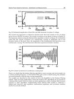
Figure 4 shows the effects of number of samples on the fundamental component magnitude
using the three techniques at a sampling frequency = 1620 Hz and the measurement set is
corrupted with a noise having standard deviation of 0.1 Gaussian distribution.

Fig. 4. Effect of number of samples on the magnitude estimation of the fundamental
harmonic (sampling frequency = 1620 Hz).
It can be noticed from this figure that the DFT algorithm gives an essentially exact estimate
of the fundamental voltage magnitude. The LAV algorithm requires a minimum number of
samples to give a good estimate, while the LES gives reasonable estimates over a wide range
of numbers of samples. However, the performance of the LAV and LES algorithms is
improved when the sampling frequency is increased to 1800 Hz as shown in Figure 5.
Figure 6 –9 gives the same estimates at the same conditions for the 5
th
, 7
th
, 11
th
and 13
th

harmonic magnitudes. Examining these figures reveals the following remarks.

For all harmonics components, the DFT gives bad estimates for the magnitudes. This
bad estimate is attributed to the phenomenon known as “spectral leakage” and is due to
the fact that the number of samples per number of cycles is not an integer.

As the number of samples increases, the LES method gives a relatively good performance.
The LAV method gives better estimates for most of the number of samples.

At a low number of samples, the LES produces poor estimates.

However, as the sampling frequency increased to 1800 Hz, no appreciable effects have
changed, and the estimates of the harmonics magnitude are still the same for the three
techniques.

Power Quality Harmonics Analysis and Real Measurements Data

16

Fig. 5. Effect of number of samples on the magnitude estimation of the fundamental
harmonic (sampling frequency = 1800 Hz).

Fig. 6. Effect of number of samples on the magnitude estimation of the 5
th
harmonic
(sampling frequency = 1620 Hz).

Electric Power Systems Harmonics - Identification and Measurements

17


Fig. 7. Effect of number of samples on the magnitude estimation of the 7
th
harmonic
(sampling frequency = 1620 Hz).


Fig. 8. Effect of number of samples on the magnitude estimation of the 11
th
harmonic

(sampling frequency = 1620 Hz).

Power Quality Harmonics Analysis and Real Measurements Data

18

Fig. 9. Effect of number of samples on the magnitude estimation of the 13
th
harmonic
(sampling frequency = 1620 Hz).
The CPU time is computed for each of the three algorithms, at a sampling frequency of 1620
Hz. Figure 10 gives the variation of CPU.


Fig. 10. The CPU times of the LS, DFT, and LAV methods (sampling frequency = 1620 Hz).

Electric Power Systems Harmonics - Identification and Measurements

19
The CPU time for the DFT and LES algorithms are essentially the same, and that of the LAV
algorithm is larger. As the number of samples increases, the difference in CPU time between
the LAV and LS/DFT algorithm increases.
Other interesting studies have been carried out on the performance of the three algorithms
when 10% of the data is missed, taken uniformly at equal intervals starting from the first
data point, for the noise free signal and 0.1 standard deviation added white noise Gaussian,
and the sampling frequency used is 1620 Hz.
Figure 11 gives the estimates of the three algorithms at the two cases. Examining this figure
we can notice the following remarks:
For the no noise estimates, the LS and DFT produce bad estimates for the fundamental
harmonic magnitude, even at a higher number of samples

The LAV algorithm produces good estimates, at large number of samples.


Fig. 11. Effect of number of samples on the magnitude estimation of the fundamental
harmonic for 10% missing data (sampling frequency = 1620 Hz): (a) no noise; (b) 0.1
standard deviation added white Gaussian noise.

Power Quality Harmonics Analysis and Real Measurements Data

20
Figure 12 –15 give the three algorithms estimates, for 10% missing data with no noise and
with 0.1 standard deviation Gaussian white noise, when the sampling frequency is 1620 Hz
for the harmonics magnitudes and the same discussions hold true.
3.4 Remarks
Three signal estimation algorithms were used to estimate the harmonic components of the
AC voltage of a three-phase six-pulse AC-DC converter. The algorithms are the LS, LAV,
and DFT. The simulation of the ideal noise-free case data revealed that all three methods
give exact estimates of all the harmonics for a sufficiently high sampling rate. For the noisy
case, the results are completely different. In general, the LS method worked well for a high
number of samples. The DFT failed completely. The LAV gives better estimates for a large
range of samples and is clearly superior for the case of missing data.




Fig. 12. Effect of number of samples on the magnitude estimation of the 5
th
harmonic for
10% missing data (sampling frequency = 1620 Hz): (a) no noise; (b) 0.1 standard deviation
added white Gaussian noise.

Electric Power Systems Harmonics - Identification and Measurements

21

Fig. 13. Effect of number of samples on the magnitude estimation of the 7
th
harmonic for
10% missing data (sampling frequency = 1620 Hz): (a) no noise; (b) 0.1 standard deviation
added white Gaussian noise.
4. Estimation of harmonics; the dynamic case
In the previous section static-state estimation algorithms are implemented for identifying
and measuring power system harmonics. The techniques used in that section was the least
error squares (LES), least absolute value (LAV) and the recursive least error squares
algorithms. These techniques assume that harmonic magnitudes are constant during the
data window size used in the estimation process. In real time, due to the switching on-off of
power electronic equipments (devices) used in electric derives and power system
transmission (AC/DC transmission), the situation is different, where the harmonic
magnitudes are not stationary during the data window size. As such a dynamic state
estimation technique is required to identifying (tracking) the harmonic magnitudes as well
as the phase angles of each harmonics component.
In this section, we introduce the Kalman filtering algorithm as well as the dynamic least
absolute value algorithm (DLAV) for identifying (tracking) the power systems harmonics
and sub-harmonics (inter-harmonics).
The Kalman filtering approach provides a mean for optimally estimating phasors and the
ability to track-time-varying parameters.
The state variable representation of a signal that includes n harmonics for a noise-free
current or voltage signal s(t) may be represented by [7]

   

1
cos
n
ii
i
st A t i t





(37)
where
A
i
(t) is the amplitude of the phasor quantity representing the ith harmonic at time t

i
is the phase angle of the ith harmonic relative to a reference rotating at i


n is the harmonic order
Each frequency component requires two state variables. Thus the total number of state
variable is 2n. These state variables are defined as follows

Power Quality Harmonics Analysis and Real Measurements Data

22

   

   
 
11 1 21 1
22 2 3 1 2
21
cos , sin
cos , 2 sin


cos ,
nnn
xt At xt At
xt At xt A t
xtAt











 
22
sin
nn
xt At



, (38)
These state variables represent the in-phase and quadrate phase components of the
harmonics with respect to a rotting reference, respectively. This may be referred to as model
1. Thus, the state variable equations may be expressed as:

11
1 0 0
0 1 0
22

0 0 1 0
21 21
0 0 1
2
xx
xx
xx
nn
xx
n














 






  


1
2

21
22
w
k
n
nn
















(39)
or in short hand







1Xk Xk wk

  (40)
where
X is a 2n  1 state vector

Is a 2n  2n state identity transition matrix, which is a diagonal matrix
w(k) is a 2n  1 noise vector associated with the transition of a sate from k to k + 1 instant
The measurement equation for the voltage or current signal, in this case, can be rewritten as,
equation (37)

   

1
2
21
2
cos sin cos sin
n
n
k
x
x
s k t wk t wk t nwk t nwk t v k
x
x





     






(41)
which can be written as










Zk HkXk vk
(42)
where Z(k) is m  1 vector of measurements of the voltage or current waveforms, H(k) is m 
2n measurement matrix, which is a time varying matrix and v(k) is m  1 errors
measurement vector. Equation (40) and (42) are now suitable for Kalman filter application.
Another model can be derived of a signal with time-varying magnitude by using a
stationary reference, model 2. Consider the noise free signal to be

   
cos
kk
st At wt



(43)

Electric Power Systems Harmonics - Identification and Measurements

23
Now, consider







1
cos
kk
xk At wt


 and


2
xk to be




sin
kk
At wt


. At t
k+2
, which
is t
k
+ t, the signal may be expressed as









 
11 1
11 2
cos 1
1cos sin
kk k
st At wt w t x k
x k x k wt x k wt



  
  

also







21

12
1sin
sin cos
kk
xk At wt wt
x k wt x k wt


 

 

Thus, the state variable representation takes the following form







111
222
1
cos sin

sin cos
1
xk xk wk
wt wt
wt wt

xk xk wk



 












(44)
and the measurement equation then becomes






1
2
1 0
xk
Zk vk

xk





(45)
If the signal includes n frequencies; the fundamental plus n – 1 harmonics, the state variable
representation may be expressed as









11
1
22
21 21
22
11
0
11



11

0
11
nn
n
nn
xk xk
M
xk xk
xk xk
M
xk xk

 

 


 

 


 

 


 



 
 

 

 



1
2
21
2

n
n
wk




















(46)
where the sub-matrices M
i
are given as

cos sin
sin cos
i
iw t iw t
M
iw t iw t











,
1, ,in



(47)
Equation (46) can be rewritten as

 
1Xk kXk wk

 
(48)
while equation (45) as

  
Zk HXk Vk
(49)
This model has constant state transition and measurement matrices. However, it assumes a
stationary reference. Thus, the in-phase and quadrature phase components represent the
instantaneous values of con-sinusoidal and sinusoidal waveforms, respectively.

Power Quality Harmonics Analysis and Real Measurements Data

24
4.1 Testing the kalman filter algorithm
The two Kalman filter models described in the preceding section were tested using a
waveform with known harmonic contents. The waveform consists of the fundamental, the
third, the fifth, the ninth, the eleventh, the thirteenth, and the nineteenth harmonics. The
waveform is described as








  

1.0 cos 10 0.1cos 3 20 0.08cos 5 30
0.08cos 7 40 0.06 cos 11 50
0.05cos 13 60 0.03cos 19 70
st t t t
tt
tt
 


  
 
 
 



The sampling frequency was selected to be 64  60 Hz.
i.
Initial process vector
As the Kalman filter model started with no past measurement, the initial process vector
was selected to be zero. Thus, the first half cycle (8 milliseconds) is considered to be the
initialization period.
ii.
Initial covariance matrix

The initial covariance matrix was selected to be a diagonal matrix with the diagonal
values equal to 10
p.u.
iii.
Noise variance (R)
The noise variance was selected to be constant at a value of 0.05 p.u.
2
. This was passed
on the background noise variance at field measurement.
iv.
State variable covariance matrix (Q)
The matrix Q was also selected to be 0.05 p.u.
Testing results of model 1, which is a 14-state model described by equations (40) and (42) are
given in the following figures. Figure 14 shows the initialization period and the recursive
estimation of the magnitude of the fundamental and third harmonic.
Figure 15 shows the
Kalman gain for the fundamental component. Figure 16 shows the first and second diagonal
element of P
k
.


Fig. 14. Estimated magnitudes of 60 Hz and third harmonic component using the 14-state
model 1.

Electric Power Systems Harmonics - Identification and Measurements

25

Fig. 15. Kalman gain for x

1
and x
2
using the 14-state model 1.


Fig. 16. The first and second diagonal elements of P
k
matrix using the 14-state model 1.
While the testing results of model 2 are given in Figures 26 –28. Figure 26 shows the first
two components of Kalman gain vector. Figure 27 shows the first and second diagonal
elements of P
k
. The estimation of the magnitude of and third harmonic were exactly the
same as those shown in Figure 23.


Fig. 17. Kalman gain for x
1
and x
2
using the 14-state model 2.

Power Quality Harmonics Analysis and Real Measurements Data

26

Fig. 18. The first and second diagonal elements of P
k
matrix using the 14-state model 2.

The Kalman gain vector K
k
and the covariance matrix P
k
reach steady-state in about half a
cycle, when model 1 is used, 1/60 seconds. Its variations include harmonics of 60 Hz. The
covariance matrix in the steady-state consists of a constant plus a periodic component. These
time variations are due to the time-varying vector in the measurement equation. Thus, after
initialization of the model, the Kalman gain vector of the third cycle can be repeated for
successive cycles.
When model 2 is selected, the components of the Kalman gain vector and the covariance
matrix become constants. In both models, the Kalman gain vector is independent of the
measurements and can be computed off-line. As the state transition matrix is a full matrix, it
requires more computation than model 1 to update the state vector.
Kalman filter algorithm is also tested for actual recorded data. Two cases of actual recorded
data are reported here. The first case represents a large industrial load served by two parallel
transformers totaling 7500 KVA [5]. The load consists of four production lines of induction
heating with two single-phase furnaces per line. The induction furnaces operate at 8500 Hz
and are used to heat 40-ft steel rods which are cut into railroad spikes. Diodes are used in the
rectifier for converting the 60 Hz power into dc and SCRs are used in the inverter for
converting the dc into single-phase 8500 Hz power. The waveforms were originally sampled at
20 kHz. A program was written to use a reduced sampling rate in the analysis. A careful
examination of the current and voltage waveforms indicated that the waveforms consist of (1)
harmonics of 60 Hz and (2) a decaying periodic high-frequency transients. The high-frequency
transients were measured independently for another purpose [6]. The rest of the waveform
was then analyzed for harmonic analysis. Using a sampling frequency that is a multiple of 2
kHz, the DFT was then applied for a period of 3 cycles. The DFT results were as follows:

Freq. (Hz) Mag. Angle (rad.)
60 1.0495 -0.20

300 0.1999 1.99
420 0.0489 -2.18
660 0.0299 0.48
780 0.0373 2.98
1020 0.0078 -0.78
1140 0.0175 1.88

Electric Power Systems Harmonics - Identification and Measurements

27

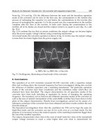
Fig. 19. Actual recorded current waveform of phases A, B, and C.
The Kalman filter, however, can be applied for any number of samples over a half cycle. If
the harmonic has time-varying magnitude, the Kalman filter algorithm would track the time
variation after the initialization period (half a cycle). Figures 19 and 20 show the three-phase
current and voltage waveforms recorded at the industrial load. Figures 21 –23 show the
recursive estimation of the magnitude of the fundamental, fifth, and seventh harmonics; the
eleventh and thirteenth harmonics; and the seventeenth and nineteenth harmonics,
respectively, for phase A current. The same harmonic analysis was also applied to the actual
recorded voltage waveforms. Figure 24 shows the recursive estimation of the magnitude of
the fundamental and fifth harmonic for phase A voltage. No other voltage harmonics are
shown here due tot he negligible small value.


Fig. 20. Actual recorded voltage waveform of phase A, B, and C.

Power Quality Harmonics Analysis and Real Measurements Data

28

Fig. 21. Estimated magnitudes of the fundamental, fifth, and seventh harmonics for phase A
current.


Fig. 22. Estimated magnitudes of the eleventh and thirteenth harmonics for phase A current.


Fig. 23. Estimated magnitudes of the seventeenth and nineteenth harmonics for phase A
current.