Bishop, Robert H. - The Mechatronics Handbook [CRC Press 2002] Part 3 doc
Bạn đang xem bản rút gọn của tài liệu. Xem và tải ngay bản đầy đủ của tài liệu tại đây (156.83 KB, 4 trang )
and associated mass moments of inertia are given in Fig. 9.13. General rigid bodies are discussed in
section “Inertia Properties.”
There are several useful concepts and theorems related to the properties of rigid bodies that can be
helpful at this point. First, if the mass moment of inertia is known about an axis through its center of
mass (I
G
), then Steiner’s theorem (parallel axis theorem) relates this moment of inertia to that about
another axis a distance d away by I = I
G
+ md
2
, where m is the mass of the body. It is also possible to
build a moment of inertia for composite bodies, in those situations where the individual motion of each
body is negligible. A useful concept is the radius of gyration, k, which is the radius of an imaginary
cylinder of infinitely small wall thickness having the same mass, m, and the same mass moment of inertia,
I, as a body in question, and given by, k = . The radius of gyration can be used to find an equivalent
mass for a rolling body, say, using m
eq
= I/k
2
.
Coupling Mechanisms
Numerous types of devices serve as couplers or power transforming mechanisms, with the most common
being levers, gear trains, scotch yokes, block and tackle, and chain hoists. Ideally, these devices and their
analogs in other energy domains are power conserving, and it is useful to represent them using a 2-port
model. In such a model element, the power in is equal to the power out, or in terms of effort-flow pairs,
e
1
f
1
= e
2
f
2
. It turns out that there are two types of basic devices that can be represented this way, based
on the relationship between the power variables on the two ports. For either type, a relationship between
two of the variables can usually be identified from geometry or from basic physics of the device. By
imposing the restriction that there is an ideal power-conserving transformation inherent in the device,
a second relationship is derived. Once one relation is established the device can usually be classified as
a transformer or gyrator. It is emphasized that these model elements are used to represent the ideal
power-conserving aspects of a device. Losses or dynamic effects are added to model real devices.
A device can be modeled as a transformer when e
1
= me
2
and mf
1
= f
2
. In this relation, m is a
transformer modulus defined by the device physics to be constant or in some cases a function of states of the
system. For example, in a simple gear train the angular velocities can be ideally related by the ratio of pitch
radii, and in a slider crank there can be formed a relation between the slider motion and the crank angle.
Consequently, the two torques can be related, so the gear train is a transformer. A device can be modeled
as a gyrator if e
1
= rf
2
and rf
1
= e
2
, where r is the gyrator modulus. Note that this model can represent
FIGURE 9.13 Mass moments of inertia for some common bodies.
2
Jmr
Pointmassatradiusr
Rod or bar about centroid
c
c
Cylinder about axis c-c
(radius r)
L
2
12
mL
J
2
1
2
Jmr
d
L
22
(4)
12
m
Jdl
Short bar about pivot
c
c
Cylindrical shell
about axis c -c
(inner radius r)
2
Jmr
Slender bar case, d=0
If outer radius is R,and
not a thin shell,
22
1
2
( )
JmRr
I/m
©2002 CRC Press LLC
10
Fluid Power Systems
10.1 Introduction
Fluid Power Systems • Electrohydraulic
Control Systems
10.2 Hydraulic Fluids
Density • Viscosity • Bulk Modulus
10.3 Hydraulic Control Valves
Principle of Valve Control • Hydraulic Control Valves
10.4 Hydraulic Pumps
Principles of Pump Operation • Pump Controls
and Systems
10.5 Hydraulic Cylinders
Cylinder Parameters
10.6 Fluid Power Systems Control
System Steady-State Characteristics • System Dynamic
Characteristics • E/H System Feedforward-Plus-PID
Control • E/H System Generic Fuzzy Control
10.7 Programmable Electrohydraulic Valves
10.1 Introduction
Fluid Power Systems
A fluid power system uses either liquid or gas to perform desired tasks. Operation of both the liquid
systems (hydraulic systems) and the gas systems (pneumatic systems) is based on the same principles.
For brevity, we will focus on hydraulic systems only.
A fluid power system typically consists of a hydraulic pump, a line relief valve, a proportional direction
control valve, and an actuator (Fig. 10.1). Fluid power systems are widely used on aerospace, industrial,
and mobile equipment because of their remarkable advantages over other control systems. The major
advantages include high power-to-weight ratio, capability of being stalled, reversed, or operated inter-
mittently, capability of fast response and acceleration, and reliable operation and long service life.
Due to differing tasks and working environments, the characteristics of fluid power systems are
different for industrial and mobile applications (Lambeck, 1983). In industrial applications, low noise
level is a major concern. Normally, a noise level below 70 dB is desirable and over 80 dB is excessive.
Industrial systems commonly operate in the low (below 7 MPa or 1000 psi) to moderate (below 21 MPa
or 3000 psi) pressure range. In mobile applications, the size is the premier concern. Therefore, mobile
hydraulic systems commonly operate between 14 and 35 MPa (2000–5000 psi). Also, their allowable
temperature operating range is usually higher than in industrial applications.
Qin Zhang
University of Illinois
Carroll E. Goering
University of Illinois
©2002 CRC Press LLC
11
Electrical Engineering
11.1 Introduction
11.2 Fundamentals of Electric Circuits
Electric Power and Sign Convention • Circuit Elements and
Their
i-v
Characteristics • Resistance and Ohm’s Law
• Practical Voltage and Current Sources • Measuring Devices
11.3 Resistive Network Analysis
The Node Voltage Method • The Mesh Current Method
• One-Port Networks and Equivalent Circuits • Nonlinear
Circuit Elements
11.4 AC Network Analysis
Energy-Storage (Dynamic) Circuit Elements • Time-
Dependent Signal Sources • Solution of Circuits Containing
Dynamic Elements • Phasors and Impedance
11.1 Introduction
The role played by electrical and electronic engineering in mechanical systems has dramatically increased
in importance in the past two decades, thanks to advances in integrated circuit electronics and in materials
that have permitted the integration of sensing, computing, and actuation technology into industrial
systems and consumer products. Examples of this integration revolution, which has been referred to as
a new field called
Mechatronics
, can be found in consumer electronics (auto-focus cameras, printers,
microprocessor-controlled appliances), in industrial automation, and in transportation systems, most
notably in passenger vehicles. The aim of this chapter is to review and summarize the foundations of
electrical engineering for the purpose of providing the practicing mechanical engineer a quick and useful
reference to the different fields of electrical engineering. Special emphasis has been placed on those topics
that are likely to be relevant to product design.
11.2 Fundamentals of Electric Circuits
This section presents the fundamental laws of circuit analysis and serves as the foundation for the study
of electrical circuits. The fundamental concepts developed in these first pages will be called on through
the chapter.
The fundamental electric quantity is
charge
, and the smallest amount of charge that exists is the charge
carried by an electron, equal to
(11.1)
As you can see, the amount of charge associated with an electron is rather small. This, of course, has
to do with the size of the unit we use to measure charge, the
coulomb
(C), named after Charles Coulomb.
However, the definition of the coulomb leads to an appropriate unit when we define electric current,
q
e
1.602 10
19–
coulomb×–=
Giorgio Rizzoni
Ohio State University
©2002 CRC Press LLC