Control of Redundant Robot Manipulators - R.V. Patel and F. Shadpey Part 5 pptx

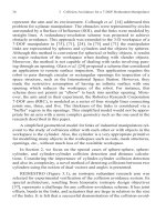
3.3
Kinemati
c Si
mul
ati
on for a 7-DOF Redun
dant
Manipulator
51
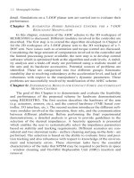
Figure 3.10 Cylinder-Sphere Collision Detection
3.3 Kinematic Simulation for a 7-DOF
Redundant Manipulator
In this section, the redundancy-resolution scheme described in Chapter
2 is extended for the general case of a 7-DOF redundant manipulator work-
ing in a 3-D workspace and applied to REDIESTRO. The feasibility of the
algorithms is illustrated using a kinematic simulation
w
R
j
p
i
u
ij
p
ij
h
ij
C
i
R
i

p
j
S
j
H
i
B
i
P
i
T
i
P
j
e
i
L
i
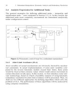
Figure 3.11 Sphere-Sphere Collision Detection
3.3.1 Kinematics of REDIESTRO
The kinematic description of REDIESTRO (a photograph of REDI-
ESTRO is shown in Figure 3.1 is obtained by assigning a coordinate frame
to each link with its z axis along the axis of rotation. Frame {1} is the work-
space fixed frame and frame {8} is the end-effector frame. Two consecu-
tive frames {i} and {i+1} are related by the homogenous
transformation matrix:
R
i
S
i

R
j
W
P
i
u
ij
h
ij
P
j
44
T
i
i 1+

i
cos 
i

i
sincos– 
i

i
sinsin a
i

i
cos


i
sin 
i

i
coscos 
i

i
cossin– a
i

i
sin
0 
i
sin 
i
cos b
i
00 01
=
52 3 Collision Avoidance for a 7-DOF Redundant Manipulator
3.3
Kinemati
c Si
mul
ati
on for a 7-DOF Redun

dant
Manipulator
53
(3.3.1)
where ;,,, and are the twist angle, joint angle, offset
and link length, respectively. The Denavit-Hartenberg parameters of REDI-
ESTRO are given in Table A-1 ( ). The homogenous transformation relat-
ing Frame 8 (end-effector frame) to the base frame is given by:
(3.3.2)
3.3.2 Main Task Tracking
The main task is described by the pose (position and orientation) of the
end-effector, defined by the position vector and the rotation
matrix of the transformation matrix . The pose is thus
dimensionally non-homogenous and needs different treatment for the 3-
dimensional vector representing the end-effector position from the
rotation matrix representing orientation. Therefore, the main task is divided
into two independent sub-tasks.
3.3.2.1 Position Tracking
The position is described in the workspace-fixed reference frame. Both
the desired and the actual position are described in this frame. The ith col-
umn of the Jacobian corresponding to the position of the end-effector in
frame {1} is defined by
(3.3.3)
where is the unit vector along the Z axis of joint i ,is the position of
the end-effector, andis the position of the origin of the ith frame
with respect to frame {1} . The position and the velocity errors are given by
(3.3.4)
where is the vector of joint velocities, and the superscript d denotes the
desired values.
R

i
i 1+

33
P
i
i 1+

31
01
i 17==
i 17= 
i

i
b
i
a
i
T
1
8
T
1
2
T 
2
3
T
7

8
=
P
1
8

31
R
1
8

33
T
1
8
33
J
P
e
i
31
Z
ˆ
1
i
P
1
8 origin
P
1

iorigin
– i 17==
Z
ˆ
1
i
P
1
8
P
1
iorigin
e
p
P
1 d
8
P
1
8
e
·
p
– J
P
e
q
·
P
·

1 d
8
–==
q
·
3.3.2.2Orientation Tracking
called the Direction Cosine matrix. The it
h
column of the Jacobian
matrix, which relates the angular velocity of the end-effector () to the
joint velocity, i.e., , can be calculated from the relation
(3.3.5)
The procedure for finding the orientation error and itsderivative is
more complicated than that for the case of position. In this case, the desired
orient
ation is described by a
mat
rix whose columns ar
e unit vectors
coincident with the desired x, y, and z axes of the end-effector. The actual
orient
ation
of
the end-effector is given
by the
matrix
. The
orient
ation
error is calculated as follows [42]:

, where
and
are
the axis and angle of rotation which transform the end-effector frame to the
desired orientation. The calculation
of
the angular
velocity error
is straight-
forward:
(3.3.6)
3.3.2.3Simulation Results
The performance of redundancy resolution in tracking the main task
trajectories is studied here by computer simulation. The integration step
size in the following simulations is 10 ms, and the main task consists of
tracking the position and orientation trajectories, generated by linear inter-
polation between the initial and final poses. It should be noted that interpo-
lation of rotations is a much more co
mplex problem than point interpolation
in
.
Sophisticated algorithms have b
een proposed in the
literature for
this purpose, e.g., see [22], [79], bu
t
these are not intended for
real-time
implementation. For this reason, we
use simple linear interpolation for both

translation and rotation, which nevertheless leads to satisfactory results.
The initial and final poses are specified below:
The orientation of the end-effector is represented by the matrix
33
R
1
8

1
e

1
e
J
O
e
q
·
=
J
O
e
i Z
ˆ
1
i
i 17==
33
R
1

8
e
O
K
1
sin= K
1

e
·
O

d
1
e
J
O
e
q
·
–=
IR
3
54 3 Collision Avoidance for a 7-DOF Redundant Manipulator
3.3
Kinemati
c Si
mul
ati
on for a 7-DOF Redun

dant
Manipulator
55
where . The overall redundancy-resolution scheme has not been
changed (see S
ection
2.3.1.3 ). The
only dif
ference
consists of splitting the
main task into two independent sub-tasks with weighting matrices denoted
by
and
corresponding to position and orientation respectively
of
the end-ef
fector
.
The joint velocities are calculated from
(3.3.7)
where
(3.3.8)
(3.3.9)
The subscript c refers to the additional task which is not active in the simu-
lation presented
in this section. It
shou
ld
be
noted in th

e following
si
mula-
tions that redundancy resolution is implemented in closed-loop. Hence, the
reference velocities are given by:
(3.3.10)
(3.3.1
1)
where and are the position and orientation proportional gains
respectively. In the first simulation, the sub-task corresponding to tracking
the desired orientation is inactive. a and b show the
P
1
8
dintial–
61.8
231.4
1127.1
=
P
1
8
dfinal–
50
0
500
1102.3
=
R
1

8
dfinal–
 0 
01
0
– 0 
=
R
1
8
dinitial–
0.1430.25– 0.958–
0.93– 0.30 0.22–
0.3390.921 0.19–
=
 22=
W
P
e
W
O
e
q
·
A
1–
b=
AJ
p
e

T
W
p
e
J
p
e
J
O
e
T
W
O
e
J
O
e
J
c
T
W
c
J
c
W
v
+++=
bJ
p
e

T
W
p
e
P
·
r
J
O
e
T
W
O
e

r
J
c
T
W
c
Z
·
r
++=
P
·
r
P
·

1
8
d
K
p
P
P
1
8
d
P
1
8
–+=

r

1 d
e
K
p
O
e
O
+=
K
p
P
K
p

O
Figur
e
3.12
Simulati
on results for
positi
on
and orientation tracking: (
a)
position error (m); (b) orientation error (rad)
0 0.5 1 1.5 2
-6
-4
-2
0
2
4
6
x 10
-
3
(a)
time (s)
0 0.5 1 1.5 2
-0.6
-0.4
-0.2
0
0.2

0.4
0.6
0.8
(b)
time (s)
W
P
e
10I
33
W
O
e
0 I
33
W
v
I
77
===
56 3 Collision Avoidance for a 7-DOF Redundant Manipulator
3.3
Kinemati
c Si
mul
ati
on for a 7-DOF Redun
dant
Manipulator
57

Figure 3.12 (contd.) Simulation results for position and orientation
tracking: (c) position error (mm); (d) orientation error (rad)
0 0.5 1 1.5 2
-50
0
50
100
150
200
250
300
350
400
450
(c)
time (s)
W
P
e
0 I
33
W
O
e
10I
33
W
v
I
77

===
0 0.5 1 1.5 2
-4
-3
-2
-1
0
1
2
3
4
5
6
x 10
-4
(d)
time (s)
position and orientation errors. In the second simulation only the orienta-
tion sub-task is active, and the result
s
are shown in c,d. In
this case, no
attempt has been made to follow the position trajectory. The position and
orientation errors are mainly due to the presence
of
in the damped
least-squares formulation of the redundancy resolution.
In the following simulations, both position and orientation sub-tasks
are active. a-c show the results of the simulation with small (the singu-
larity robustness factor). As we can see in a, at some point, the position and

orientation
sub-tasks are in conflict
wi
th each other. This causes the whole
Jacobian of the main task to approach a singular position where the condi-
tion number of the
Jaco
bian ma
trix
is
. Therefore, there is
considerable e
rror on both sub-tasks.
d, e, and f show the
simulation
results with a larger value of . This time, the whole Jacobian matrix
remains far from singularity (), and the maximum errors
are reduced significantly. However, in the case that , there is
considerable error at the end of the trajectory. This shows that should
be selected
as small
as possible.
Figure 3.13 (a) Condition number of matrix
W
v
W
v
Cond
max
403

=
W
v
Cond
max
105=
W
v
20I
77
=
W
v
time (s)
J
T
P
e
J
T
O
e

T
; W
v
1 I
33
=
58 3 Collision Avoidance for a 7-DOF Redundant Manipulator

3.3
Kinemati
c Si
mul
ati
on for a 7-DOF Redun
dant
Manipulator
59
Figure 3.13 (contd.) Simulation results when both main sub-tasks are
active; (a)-(c):
Figure 3.13 (contd.) (d) Condition number of matrix
0 0.5 1 1.5 2
-1
0
1
2
3
0 0.5 1 1.5 2
0
0.1
0.2
(c) Orientation
error (rad)
time (s)
ti
me
(s)
(b) Position
error (mm)

W
v
1 I
33
=
time (s)
J
T
P
e
J
T
O
e

T
;
W
v
1 I
33
=
Figure 3.13 (contd.) Simulation results when both main
sub-
tasks
are active; (d)-(f):
The isotropic design of REDIESTRO reduces the risk of approaching a
singular configuration over a greater part of the workspace. However, this
risk cannot be eliminated completely, and the singularity robustness factor
should either be selected large enough, which introduces errors in the

main task, or should be time-varying, with diagonal entries proportional to
the inverse of the minimum singular value of the “normalized” Jacobian of
the main task. The Jacobian matrix
is normalized using the concept of
char
-
acteristic length [85] to resolve the dimensional inhomogeneity in the
matrix due to the presence of positioning and orienting tasks. Figure 3.14
shows the comparison between these
two
approaches. As one can conclude,
the variable-weight formulation shows better
performance
because
has
small values far from a singular configuration. Hence, variable weights do
not introduce errors on
the main task
, and grow appropriately near a singu-
lar
configuration. While the computational complexity
of the numerical
implementation of the SVD algorithm for a 7-DOF arm may not be accept-
able for real-time control, bounds for the singular values of can be
0 0.5 1 1.5 2
0
0.5
0 0.5 1 1.5 2
0
0.2

(e) Position
error (mm)
(f) Orientation
error (rad)
time (s)
time (s)
W
v
20I
33
=
W
v
W
v
J
60 3 Collision Avoidance for a 7-DOF Redundant Manipulator
3.3
Kinemati
c Si
mul
ati
on for a 7-DOF Redun
dant
Manipulator
61
found by means of bounds on the real, non-negative eigenvalues of .
As shown in [86], these bounds can be found quite economically by resort-
ing to the Gerschgorin Theorem [89]
Figure 3.14 Comparison between the fixed and the time-varying

singularity robustness factor
3.3.3Additional Tasks
The additional tasks incorporated in the redundancy resolution module
are as follows: Joint Limit Avoidance (JLA), Stationary and Moving Obsta-
cle Collision Avoidance (SOCA, MOCA) and Self Collision Avoidance
(SCA).
JJ
T
0 0.5 1 1.5 2
0
20
40
60
80
100
0 0.5 1 1.5 2
0
0.1
0.2
0.3
 W
v
 I
77
=
Fixed W
v
,___ Variable W
v
time (s)

time (s)
Orientation Error (rad)
3.3.3.1 Joint Limit Avoidance
The JLA algorithm developed in Section 2.4.1.3 is extended here to 3-
D without major modifications. In this case, the Jacobian matrix of the JLA
corresponding to the ith joint is: , where is the ith column of
the matrix . The same weight scheduling scheme is used as that
implemented for JLA in Section 2.4.1.3 . In the following simulation, the
main task is the same as in Section 3.3.2 with both position tracking and
orienta
tion
tracking active.
Figure 3.
15
shows that with
JLA in
acti
ve, joint
4 has a minimum value equal to 67 degrees. When the JLA is active with
minimum 80 degrees for joint 4, this joint is prevented from violating its
limit while tracking the main task tr
ajectory
. The position and orientation
tracking errors converge to small values except for a short transition period
when the JLA
task becomes active.
Figure 3.15 Simulation result for JLA in the 3-D workspace with
3.3.3.2 Stationary and Moving Obstacle Collision Avoidance
A photograph of REDIESTRO, with its actual links and actuators, is
shown in Figure 3.1 , while Figure 3.16 depicts the arm with each moving

J
C
e
i
T
= e
i
I
77
0 0.5 1 1.5 2
65
70
75
80
85
90
95
100
105
110
115
JLA active ____ JLA inactive
q
4
deg
time (s)
q
4
mi
n

80=
62 3 Collision Avoidance for a 7-DOF Redundant Manipulator
3.3
Kinemati
c Si
mul
ati
on for a 7-DOF Redun
dant
Manipulator
63
element of the arm enclosed in a cylindrical primitive. The links and the
actuator units are modeled by 14 cylinders in total, the fourth link having
the maximum number of 4 sub-links. The end-effector and the tool
attached to it are enclosed in a sphere.
Figure 3.16 REDIESTRO with simplified primitives
The environment is modeled by spherical and cylindrical objects. Each
obstacle is enclosed in a cylindrical or a spherical Surface of Influence
(SOI). Note that the dimensions of the SOIs are used in distance calcula-
tion, collision detection and obstacle avoidance modules rather than the
actual dimensions of the obstacles.
Additional task formulation:
Let us assume that after performing the dis-
tance calculation, the jth sub-link of the ith link of the manipulator  or
depending on the primitive used for modeling  has the risk of collision
with the kth obstacle (or ). The critical point on the sub-link and the
obstacle ( and are ) and the critical direction () are determined
by the collision detection algorithm described in Section 3.2 . Now, the
additional task for the redundancy-resolution module is defined by:
S

ij
C
ij
S
k
C
k
P
ij
c
P
k
c
u
ij k
z
i
(3.3.12)
where is the critical distance, is the Jacobian
matrix mapping the joint rates into the velocity of the critical point of
the manipulator
, while
is the vel
ocity
of the obst
acle
k . The
desired val-
ues for the active constraints (additional tasks) are: . Note
that we still need to calculate the Jacobian of the active constraints. First,

the Jacobian of the critical point is calculated, i.e.,
(3.3.13)
The kth column of the matrix
is
given by:
(3.3.14)
where is the unit vector in the direction of rotation of the kth joint,
is the position
vector of the origin of the
kth
local fr
ame.
Not
e,
t
ha
t
all variables are defined in frame {1} . Further, the Jacobian of the additional
task to be used
by the
redundancy-resolution module i
s calcul
ated
as:
(3.3.15)
Analysis:
The performance of the obstacle avoidance scheme
has been
studied by various simulations for different scenarios. As an example, the
simulation results for MOCA are illustrated in Figure 3.17 . In these simu-

lations, the main task consists of ke
eping the position of the end-ef
fector
constant while avoiding collisions with a moving object. Figure 3.17 shows
the results of the simulations for different constant values of the weighting
matrix corresponding to th
e
collision
avoidance
task.
It should
be noted
that
when Wc is too small, the object collides with the arm. When is large
enough, no coll
isi
on occurs, but there
is
a r
ap
id increase in the joi
nt veloci-
ties which results in a large pulse in joint accelerations (see Figure 3.17 ). In
a practical implementation, the maximum acceleration of each joint would
be limi
ted and this commanded joint acceleration would result in saturation
of the actuators.
z
ik
h

ij k
z
·
ij k
 u–
ij k
T
J
ij
c
q
·
p
·
k
c
–==
h
ij k
J
ij
c
q
·
p
·
ij
c
q
·


q
·
P
ij
c
p
·
k
c
z
i
d
z
·
i
d
0==
J
ij
c
J
3 i
0
37i–
=
J
Jk
31
a

ˆ
k
p
ij
c
p
korigin
– k 1 i==
a
ˆ
k
p
kori
gi
n
J
c
u
ij k
T
– J
ij
c
=
W
C
64 3 Collision Avoidance for a 7-DOF Redundant Manipulator
3.3
Kinemati
c Si

mul
ati
on for a 7-DOF Redun
dant
Manipulator
65
Figure 3.17 Simulation results for MOCA with fixed weighting factors:
(a) Critical distance (mm); (b) 2-norm of joint velocities (rad/s)
mm and SOI = 100 mm
- - - , ___ ,
(collision occurred)
R
o
70=
W
c
0.01= W
c
110
4–
=
W
c
110
5–
=
time (s)
0 0.5 1 1.5 2 2.5 3 3.5 4
60
70

80
90
100
110
120
130
140
150
()
Boundary of the object
time (s)
(a)
0 0.5 1 1.5 2 2.5 3 3.5 4
0
0
.05
0.1
0
.15
0.2
0
.25
0.3
0
.35
0.4
0
.45
()
time (s)

(b)