Control of Robot Manipulators in Joint Space - R. Kelly, V. Santibanez and A. Loria Part 11 doc
Bạn đang xem bản rút gọn của tài liệu. Xem và tải ngay bản đầy đủ của tài liệu tại đây (330.95 KB, 30 trang )
13.1 P“D” Control with Gravity Compensation
293
A possible modification to the PD control law with gravity compensation
consists in replacing the derivative part (D), which is proportional to the
˙
˜
˙
˙
derivative of the position error, i.e. to the velocity error q = q d − q, by a
term proportional to
˙
qd − ϑ
where ϑ ∈ IRn is, as said above, the result of filtering the position q by means
of a dynamic system of first-order and of zero relative degree.
Specifically, the P“D” control law with gravity compensation is written as
˙
˜
τ = Kp q + Kv [q d − ϑ] + g(q)
˙
x = −Ax − ABq
ϑ = x + Bq
(13.2)
(13.3)
where Kp , Kv ∈ IRn×n are diagonal positive definite matrices, A = diag{ai }
and B = diag{bi } and ai and bi are real strictly positive constants but otherwise arbitrary for i = 1, 2, · · · , n.
Figure 13.1 shows the block-diagram corresponding to the robot under
P“D” control with gravity compensation. Notice that the measurement of the
˙
joint velocity q is not required by the controller.
g(q)
τ
Σ
Kv
˙
qd
qd
B
Kp
ϑ Σ
Σ
q
ROBOT
(pI +A)−1AB
Σ
Figure 13.1. Block-diagram: P“D” control with gravity compensation
Define ξ = x + Bq d . The equation that describes the behavior in closed
loop may be obtained by combining Equations (III.1) and (13.2)–(13.3), which
˜ ˙
may be written in terms of the state vector ξ T q T q T
T
as
294
P“D” Control
⎡ ⎤ ⎡
⎤
˙
−Aξ + AB˜ + B q d
q
ξ
⎥
d ⎢ ⎥ ⎢
⎢ ⎥ ⎢
⎥
˙
˜
˜
q
⎢q⎥ = ⎢
⎥.
dt ⎣ ⎦ ⎣
⎦
˙
˜
˙
˙
ă
q
q
q d M (q)1 [Kp q + Kv [q d − ξ + B˜ ] − C(q, q)q]
T
˙T
˜ ˜
A sufficient condition for the origin ξ T q T q
= 0 ∈ IR3n to be a
unique equilibrium point of the closed-loop equation is that the desired joint
position q d be a constant vector. In what is left of this section we assume that
this is the case. Notice that in this scenario, the control law may be expressed
as
bi p
˜
q + g(q),
τ = Kp q − Kv diag
p + ai
which is close to the PD with gravity compensation control law (7.1), when
the desired position q d is constant. Indeed the only difference is replacement
˙
of the velocity q by
bi p
q,
diag
p + ai
˙
thereby avoiding the use of the velocity q in the control law.
As we show in the following subsections, P“D” control with gravity compensation meets the position control objective, that is,
lim q(t) = q d
t→∞
where q d ∈ IRn is any constant vector.
Considering the desired position q d as constant, the closed-loop equation
˜ ˙
may be rewritten in terms of the new state vector ξ T q T q T
⎡ ⎤ ⎡
ξ
⎢ ⎥ ⎢
d ⎢ ⎥ ⎢
˜
⎢q⎥ = ⎢
dt ⎣ ⎦ ⎣
˙
q
T
as
⎤
−Aξ + AB˜
q
⎥
⎥
⎥
⎦
˙
−q
(13.4)
˜
˜ ˙ ˙
˜
M (q d − q )−1 [Kp q − Kv [ξ − B˜ ] − C(q d − q , q)q]
q
which, in view of the fact that q d is constant, constitutes an autonomous
T
˜ ˙
= 0 ∈ IR3n is the
differential equation. Moreover, the origin ξ T q T q T
unique equilibrium of this equation.
With the aim of studying the stability of the origin, we consider the Lyapunov function candidate
1
1
T
˜
˜
˜ ˙
˙
q
q
V (ξ, q , q) = K(q, q) + q TKp q + (ξ − B˜ ) Kv B −1 (ξ − B˜ )
2
2
(13.5)
13.1 P“D” Control with Gravity Compensation
295
˙
˙
˙
where K(q, q) = 1 q TM (q)q is the kinetic energy function corresponding to
2
the robot. Notice that the diagonal matrix Kv B −1 is positive definite. Con˜ ˙
sequently, the function V (ξ, q , q) is globally positive definite.
The total time derivative of the Lyapunov function candidate yields
1
˙
˙
˜ ˙
˙
˜
˙ ˜
˙ ˙
V (ξ, q , q) = q TM (q)ă + q T M (q)q + q TKp q
q
2
T
˙
˙
˜
+ [ξ − B˜ ] Kv B −1 ξ − B q .
q
˙ ˜
˙
Using the closed-loop Equation (13.4) to solve for , q and M (q)ă , and
q
canceling out some terms we obtain
T
˙
˜ ˙
q
V (ξ, q , q) = − [ξ − B˜ ] Kv B −1 A [ξ − B˜ ]
q
⎤⎡ ⎤
⎡ ⎤T ⎡
ξ
Kv B −1 A −Kv A 0
ξ
˜
˜
BKv A 0 ⎦⎣ q ⎦
= − ⎣ q ⎦ ⎣ −Kv A
˙
˙
0
0
0
q
q
where we used
˙
qT
(13.6)
1 ˙
˙ ˙
M (q) − C(q, q) q = 0 ,
2
which follows from Property 4.2.
˙
˜ ˙
Clearly, the time derivative V (ξ, q , q) of the Lyapunov function candidate
is globally negative semidefinite. Therefore, invoking Theorem 2.3, we conclude that the origin of the closed-loop Equation (13.4) is stable and that all
solutions are bounded.
Since the closed-loop Equation (13.4) is autonomous, La Salle’s Theorem
2.7 may be used in a straightforward way to analyze the global asymptotic
stability of the origin (cf. Problem 3 at the end of the chapter). Nevertheless, we present below, an alternative analysis that also allows one to show
global asymptotic stability of the origin of the state-space corresponding to
the closed-loop Equation, (13.4). This alternative method of proof, which is
longer than via La Salle’s theorem, is presented to familiarize the reader with
other methods to prove global asymptotic stability; however, we appeal to the
material on functional spaces presented in Appendix A.
˜ ˙
According to Definition 2.6, since the origin ξ T q T q T
T
= 0 ∈ IR3n is a
˜
˙
stable equilibrium, then if ξ(t)T q (t)T q(t)T → 0 ∈ IR3n as t → ∞ (for all
initial conditions), the origin is a globally asymptotically stable equilibrium.
It is precisely this property that we show next.
In the development that follows we use additional properties of the dy˙
namic model of robot manipulators. Specifically, assume that q, q ∈ Ln .
∞
Then,
T
296
ã
ã
PD Control
d
M (q) Lnìn
dt
n
C(q, q)q L .
M (q)1 ,
ă
If moreover q Ln then,
ã
d
[C(q, q)q] Ln .
∞
dt
˜ ˙
The Lyapunov function V (ξ, q , q) given in (13.5) is positive definite since
it is composed of the following three non-negative terms:
•
•
•
1 T
˙
˙
2 q M (q)q
1 T
˜
˜
2 q Kp q
T
1
−1
q
2 [ξ − B˜ ] Kv B
[ξ − B˜ ] .
q
˙
˜ ˙
Since the time derivative V (ξ, q , q) expressed in (13.6) is negative semidef˜ ˙
inite, the Lyapunov function V (ξ, q , q) is bounded along the trajectories.
Therefore, the three non-negative terms above are also bounded along trajectories. From this conclusion we have
˙ ˜
q, q , [ξ − B˜ ] ∈ Ln .
q
∞
(13.7)
Incorporating this information in the closed-loop system Equation (13.4),
˜
˜
and knowing that M (q d − q )−1 is bounded for all q d , q ∈ Ln and also that
∞
˜ ˙ ˙
˜ ˙
C(q d − q , q)q is bounded for all q d , q , q ∈ Ln , it follows that the time deriva∞
tive of the state vector is also bounded, i.e.
ă
, q , q Ln ,
(13.8)
B q ∈ Ln .
∞
(13.9)
and therefore,
Using again the closed-loop Equation (13.4), we obtain the second time
derivative of the state variables,
ă
= A + AB q
ă
q = ă
q
d
q
q (3) = −M (q)−1
M (q) M (q)−1 [Kp q − Kv [ξ − B˜ ] − C(q, q)q]
dt
d
˙
˙
˙
˜
˙ ˙
˜
+ M (q)−1 Kp q − Kv ξ − B q −
[C(q, q)q]
dt
where q (3) denotes the third time derivative of the joint position q and we
used
13.1 P“D” Control with Gravity Compensation
297
d
d
M (q)−1 = −M (q)−1
M (q) M (q)1 .
dt
dt
ă
In (13.7) and (13.8) we have already concluded that ξ, q , q, ξ, q , q ∈ Ln
∞
then, from the properties stated at the beginning of this analysis, we obtain
ă ă
, q , q (3) Ln ,
(13.10)
ă
ă
B q Ln .
∞
(13.11)
and therefore,
On the other hand, integrating both sides of (13.6) and using that
˙
˜ ˜
V (ξ, q , q ) is bounded along the trajectories, we obtain
[ξ − B˜ ] ∈ Ln .
q
2
(13.12)
Considering (13.9), (13.12) and Lemma A.5, we obtain
q
lim [ξ(t) − B˜ (t)] = 0 .
t→∞
(13.13)
Next, we invoke Lemma A.6 with f = ξ −B˜ . Using (13.13), (13.7), (13.9)
q
and (13.11), we get from this lemma
˙
˙
˜
lim ξ(t) − B q (t) = 0 .
t→∞
Consequently, using the closed-loop Equation (13.4) we get
˙
q
lim −A[ξ(t) − B˜ (t)] + B q = 0 .
t→∞
From this expression and (13.13) we obtain
˙
lim q(t) = 0 ∈ IRn .
t→∞
(13.14)
˜
Now, we show that limt→∞ q (t) = 0 ∈ IRn . To that end, we consider again
˙
Lemma A.6 with f = q. Incorporating (13.14), (13.7), (13.8) and (13.10) we
get
ă
lim q (t) = 0 .
t
Taking this into account in the closed-loop Equation (13.4) as well as
(13.13) and (13.14), we get
˜
˜
lim M (q d − q (t))−1 Kp q (t) = 0 .
t→∞
So we conclude that
˜
lim q (t) = 0 ∈ IRn .
t→∞
(13.15)
298
P“D” Control
The last part of the proof, that is, the proof of limt→∞ ξ(t) = 0 follows
trivially from (13.13) and (13.15). Therefore, the origin is a globally attractive
equilibrium point.
This completes the proof of global asymptotic stability of the origin of the
closed-loop Equation (13.4).
We present next an example with the purpose of illustrating the performance of the Pelican robot under P“D” control with gravity compensation.
As for all other examples on the Pelican robot, the results that we present are
from laboratory experimentation.
Example 13.1. Consider the Pelican robot studied in Chapter 5, and
depicted in Figure 5.2. The components of the vector of gravitational
torques g(q) are given by
g1 (q) = (m1 lc1 + m2 l1 )g sin(q1 ) + m2 lc2 g sin(q1 + q2 )
g2 (q) = m2 lc2 g sin(q1 + q2 ) .
Consider the P“D” control law with gravity compensation on this
robot for position control and where the design matrices Kp , Kv , A, B
are taken diagonal and positive definite. In particular, pick
Kp = diag{kp } = diag{30} [Nm/rad] ,
Kv = diag{kv } = diag{7, 3} [Nm s/rad] ,
A = diag{ai } = diag{30, 70} [1/s] ,
B = diag{bi } = diag{30, 70} [1/s] .
The components of the control input τ are given by
τ1 = kp q1 − kv ϑ1 + g1 (q)
˜
˜
τ2 = kp q2 − kv ϑ2 + g2 (q)
x1 = −a1 x1 − a1 b1 q1
˙
x2 = −a2 x2 − a2 b2 q2
˙
ϑ1 = x1 + b1 q1
ϑ2 = x2 + b2 q2 .
The initial conditions corresponding to the positions, velocities and
states of the filters, are chosen as
q1 (0) = 0,
q1 (0) = 0,
˙
x1 (0) = 0,
q2 (0) = 0
q2 (0) = 0
˙
x2 (0) = 0 .
13.1 P“D” Control with Gravity Compensation
[rad]
0.4
0.3
0.2
0.1
0.0
299
...
...
..
..
..
..
.
1
.
.
.
.
.
.
.
..
..
..
..
..
..
..
..
..
..
...
...
...
...
...
....
....
..
....
..
.....
.....
2
...
.........
...
............
..................
...
............................................................................................................................................
...
..............................................................................................................................
...
...
.....
......
.....................
........................
..............................................................................................................................................................
.........................................................................................................................................................
.... .... .... .... .... .... .... .... .... .... .... .... .... .... .... .... .... .... .... .... .... .... .... .
... ... ... ... ... ... ... ... ... ... ... ... ... ... ... ... ... ... ... ... ... ... ... .
q
˜
q
˜
0.0587
0.0151
−0.1
0.0
0.5
1.0
1.5
2.0
t [s]
Figure 13.2. Graphs of position errors q1 (t) and q2 (t)
˜
˜
The desired joint positions are chosen as
qd1 = π/10, qd2 = π/30 [rad] .
In terms of the state vector of the closed-loop equation, the initial
state is
⎤
⎤ ⎡
⎡
⎤ ⎡
9.423
b1 π/10
⎢ ξ(0) ⎥ ⎢ b2 π/30 ⎥ ⎢ 7.329 ⎥
⎥
⎥ ⎢
⎢
⎥ ⎢
⎥
⎥ ⎢
⎢
⎥ ⎢
⎢ q (0) ⎥ = ⎢ π/10 ⎥ = ⎢ 0.3141 ⎥ .
⎢ ˜ ⎥ ⎢ π/30 ⎥ ⎢ 0.1047 ⎥
⎥
⎥ ⎢
⎢
⎥ ⎢
⎣
⎦ ⎣ 0 ⎦ ⎣ 0 ⎦
˙
q(0)
0
0
Figure 13.2 presents the experimental results and shows that the
˜
components of the position error q (t) tend asymptotically to a small
nonzero constant. Although we expected that the error would tend
to zero, the experimental behavior is mainly due to the presence of
unmodeled friction at the joints.
♦
In a real implementation of a controller on an ordinary personal computer
(as is the case of Example 13.1) typically the joint position q is sampled
periodically by optical encoders and this is used to compute the joint velocity
˙
q. Indeed, if we denote by h the sampling period, the joint velocity at the
instant kh is obtained as
˙
q(kh) =
q(kh) − q(kh − h)
,
h
d
that is, the differential operator p = dt is replaced by (1 − z −1 )/h, where z −1
−1
is the delay operator that is, z q(kh) = q(kh − h). By the same argument,
300
P“D” Control
in the implementation of the P“D” control law with gravity compensation,
(13.2)–(13.3), the variable ϑ at instant kh may be computed as
ϑ(kh) =
q(kh) − q(kh − h) 1
+ ϑ(kh − h)
h
2
where we chose A = diag{ai } = diag{h−1 } and B = diag{bi } = diag{2/h}.
13.2 P“D” Control with Desired Gravity Compensation
In this section we present a modification of PD control with desired gravity
compensation, studied in Chapter 7, and whose characteristic is that it does
˙
not require the velocity term q in its control law. The original references on
this controller are cited at the end of the chapter.
This controller, that we call here P“D” control with desired gravity compensation, is described by
˙
˜
τ = Kp q + Kv [q d − ϑ] + g(q d )
˙
x = −Ax − ABq
ϑ = x + Bq
(13.16)
(13.17)
where Kp , Kv ∈ IRn×n are diagonal positive definite matrices, A = diag{ai }
and B = diag{bi } with ai and bi real strictly positive constants but otherwise
arbitrary for all i = 1, 2, · · · , n.
Figure 13.3 shows the block-diagram of the P“D” control with desired
gravity compensation applied to robots. Notice that the measurement of the
˙
joint velocity q is not required by the controller.
g(q d )
τ
Σ
Kv
˙
qd
qd
q
B
Kp
ϑ Σ
Σ
ROBOT
(pI +A)−1AB
Σ
Figure 13.3. Block-diagram: P“D” control with desired gravity compensation
13.2 P“D” Control with Desired Gravity Compensation
301
Comparing P“D” control with gravity compensation given by (13.2)–(13.3)
with P“D” control with desired gravity compensation (13.16)–(13.17), we immediately notice the replacement of the term g(q) by the feedforward term
g(q d ).
The analysis of the control system in closed loop is similar to that from
Section 13.1. The most noticeable difference is in the Lyapunov function considered for the proof of stability. Given the relative importance of the controller
(13.16)–(13.17), we present next its complete study.
Define ξ = x + Bq d . The equation that describes the behavior in closed
loop is obtained by combining Equations (III.1) and (13.16)–(13.17), which
˜ ˙
may be expressed in terms of the state vector ξ T q T q T
T
as
⎡ ⎤⎡
⎤
˙
ξ
−Aξ + AB˜ + B q d
q
⎥
d⎢ ⎥⎢
⎢ ⎥⎢
⎥
˙
˜ =
˜
q
⎢q⎥ ⎢
⎥
dt ⎣
1
ă
q
q d M (q) [Kp q +Kv [q d −ξ+B˜ ]+g(q d )−C(q, q)q−g(q)]
q
T
˙T
˜ ˜
A sufficient condition for the origin ξ T q T q
= 0 ∈ IR3n to be a
unique equilibrium of the closed-loop equation is that the desired joint position
q d is a constant vector. In what follows of this section we assume that this is
the case. Notice that in this scenario, the control law may be expressed by
˜
τ = Kp q − Kv diag
bi p
p + ai
q + g(q d ),
which is very close to PD with desired gravity compensation control law (8.1)
when the desired position q d is constant. The only difference is the substitution
˙
of the velocity term q by
ϑ = diag
bi p
p + ai
q,
˙
thereby avoiding the use of velocity measurements q(t) in the control law.
As we show below, if the matrix Kp is chosen so that
λmin {Kp } > kg ,
then the P“D” controller with desired gravity compensation verifies the position control objective, that is,
lim q(t) = q d
t→∞
for any constant vector q d ∈ IRn .
302
P“D” Control
Considering the desired position q d to be constant, the closed-loop equa˜ ˙
tion may then be written in terms of the new state vector ξ T q T q T
⎡ ⎤⎡
ξ
⎢ ⎥⎢
d⎢ ⎥⎢
˜ =
⎢q⎥ ⎢
dt ⎣ ⎦ ⎣
−Aξ + AB˜
q
˙
−q
T
as
⎤
⎥
⎥
⎥
⎦
˜
M (q)−1 [Kp q −Kv [ξ−B˜ ]+g(q d )−C(q d −˜ , q)q−g(q d −˜ )]
q
q ˙ ˙
q
(13.18)
which, since q d is constant, is an autonomous differential equation. Since
the matrix Kp has been picked so that λmin {Kp } > kg , then the origin
˙
q
T
˜ ˙
ξT qT qT
= 0 ∈ IR3n is the unique equilibrium of this equation (see
the arguments in Section 8.2).
In order to study the stability of the origin, consider the Lyapunov function
candidate
1
T
˜ ˙
˜ ˙
q
q
q
V (ξ, q , q) = K(q d − q , q) + f (˜ ) + (ξ − B˜ ) Kv B −1 (ξ − B˜ )
2
(13.19)
where
˜ ˙
K(q d − q , q) =
1 T
˜ ˙
˙
q M (q d − q )q
2
1
˜
˜
˜
˜
f (˜ ) = U(q d − q ) − U(q d ) + g(q d )T q + q TKp q .
q
2
Notice first that the diagonal matrix Kv B −1 is positive definite. Since it
q
has been assumed that λmin {Kp } > kg , we have from Lemma 8.1 that f (˜ ) is a
˜
˜ ˙
(globally) positive definite function of q . Consequently, the function V (ξ, q , q)
is also globally positive definite.
The time derivative of the Lyapunov function candidate yields
1
˙
˙T
˙
˜ ˙
˙
˙ ˜
˜
˙ ˙
˜
V (ξ, q , q) = q TM (q)ă + q T M (q)q q g(q d − q ) + g(q d )T q
q
2
T
˙
˙
˙
˜
˜
˜
+ q TKp q + [ξ − B˜ ] Kv B −1 ξ − B q .
q
˙ ˜
˙
q
Using the closed-loop Equation (13.18) to solve for , q and M (q)ă , and
canceling out some terms, we obtain
T
˙
˜ ˙
q
V (ξ, q , q) = − (ξ − B˜ ) Kv B −1 A (ξ − B˜ )
q
⎤⎡ ⎤
⎡ ⎤T ⎡
−1
ξ
Kv B A −Kv A 0
ξ
˜
˜
= − ⎣ q ⎦ ⎣ −Kv A BKv A 0 ⎦ ⎣ q ⎦
˙
˙
0
0
0
q
q
where we used (cf. Property 4.2)
(13.20)
13.2 P“D” Control with Desired Gravity Compensation
˙
qT
303
1 ˙
˙ ˙
M (q) − C(q, q) q = 0 .
2
˙
˜ ˙
Clearly, the time derivative V (ξ, q , q) of the Lyapunov function candidate
is a globally semidefinite negative function. For this reason, according to the
Theorem 2.3, the origin of the closed-loop Equation (13.18) is stable.
Since the closed-loop Equation (13.18) is autonomous, direct application
of La Salle’s Theorem 2.7 allows one to guarantee global asymptotic stability
of the origin corresponding to the state space of the closed-loop system (cf.
Problem 4 at the end of the chapter). Nevertheless, an alternative analysis,
similar to that presented in Section 13.1, may also be carried out.
˜ ˙
Since the origin ξ T q T q T
T
= 0 ∈ IR3n is a stable equilibrium, then
˜
˙
if ξ(t)T q (t)T q(t)T → 0 ∈ IR3n when t → ∞ (for all initial conditions),
i.e. the equilibrium is globally attractive, then the origin is a globally asymptotically stable equilibrium. It is precisely this property that we show next.
In the development below we invoke further properties of the dynamic
˙
model of robot manipulators. Specifically, assuming that q, q ∈ Ln we have
T
ã
d
M (q)1 , dt M (q) Lnìn
ã
d
˙
C(q, q)q, g(q), dt g(q) ∈ Ln .
∞
The latter follows from the regularity of the functions that define M , g and
ă
C. By the same reasoning, if moreover q Ln then
∞
•
d
dt
˙ ˙
[C(q, q)q] ∈ Ln .
∞
˜ ˙
The Lyapunov function V (ξ, q , q) given in (13.19) is positive definite and
is composed of the sum of the following three non-negative terms
•
1 T
˙
˙
2 q M (q)q
˜
˜
˜ 2˜
• U(q d − q ) − U(q d ) + g(q d )T q + 1 q TKp q
•
1
2 (ξ
− B˜ ) Kv B −1 (ξ − B˜ ) .
q
q
T
˙
˜ ˙
Since the time derivative V (ξ, q , q), expressed in (13.6) is a negative
˜ ˙
semidefinite function, the Lyapunov function V (ξ, q , q) is bounded along
trajectories. Therefore, the three non-negative listed terms above are also
bounded along trajectories. Since, moreover, the potential energy U(q) of
robots having only revolute joints is always bounded in its absolute value, it
follows that
˙ ˜
(13.21)
q, q , ξ, ξ − B˜ ∈ Ln .
q
∞
Incorporating this information in the closed-loop Equation (13.18), and
˜
˜
˜
knowing that M (q d − q )−1 and g(q d − q ) are bounded for all q d , q ∈ Ln and
∞
304
P“D” Control
˜ ˙ ˙
˜ ˙
also that C(q d − q , q)q is bounded for all q d , q , q ∈ Ln , it follows that the
∞
time derivative of the state vector is bounded, i.e.
ă
, q , q ∈ Ln ,
∞
(13.22)
and therefore, it is also true that
˙
˙
˜
ξ − B q ∈ Ln .
∞
(13.23)
Using again the closed-loop Equation (13.18), we can compute the second
time derivative of the variables state to obtain
ă
= A + AB q
ă
q = ă
q
d
q
q (3) = M (q)1
M (q) M (q)1 [Kp q − Kv [ξ − B˜ ] − C(q, q)q
dt
+g(q d ) − g(q)]
d
d
˙
˙
˙
˜
˙ ˙
˜
+ M (q)−1 Kp q − Kv ξ − B q −
(C(q, q)q) + g(q)
dt
dt
where q (3) denotes the third time derivative of the joint position q and we
used
d
d
M (q)−1 = −M (q)−1
M (q) M (q)−1 .
dt
dt
ă
In (13.21) and (13.22) we concluded that ξ, q , q, ξ, q , q ∈ Ln then, from
∞
the properties stated at the beginning of this analysis, we obtain
ă ă
, q , q (3) Ln ,
(13.24)
ă
ă
B q Ln .
(13.25)
and therefore also
On the other hand, from the time derivative V (ξ, q , q), expressed in
(13.20), we get
(13.26)
ξ − B˜ ∈ Ln .
q
2
Considering next (13.23), (13.26) and Lemma A.5, we conclude that
q
lim ξ(t) − B˜ (t) = 0 .
t→∞
(13.27)
Hence, using (13.27), (13.21), (13.23) and (13.25) together with Lemma
A.6 we get
˙
˙
˜
lim ξ(t) − B q (t) = 0
t→∞
13.2 P“D” Control with Desired Gravity Compensation
305
˙
˙
˜
and consequently, taking ξ and q from the closed-loop Equation (13.18), we
get
˙
lim −A[ξ(t) − B˜ (t)] + B q = 0 .
q
t→∞
From this last expression and since we showed in (13.27) that limt→∞ ξ(t)−
B˜ (t) = 0 it finally follows that
q
˙
lim q(t) = 0 .
t→∞
(13.28)
˜
We show next that limt→∞ q (t) = 0 ∈ IRn . Using again Lemma A.6 with
(13.28), (13.21), (13.22) and (13.24) we have
ă
lim q (t) = 0 .
t
Taking this into account in the closed-loop Equation (13.18) as well as
(13.27) and (13.28), we get
˜
˜
˜
lim M (q d − q (t))−1 [Kp q (t) + g(q d ) − g(q d − q (t))] = 0
t→∞
and therefore, since λmin {Kp } > kg we finally obtain from the methodology
presented in Section 8.2,
˜
lim q (t) = 0 .
(13.29)
t→∞
The rest of the proof, that is that limt→∞ ξ(t) = 0, follows directly from
(13.27) and (13.29).
This completes the proof of global attractivity of the origin and, since we
have already shown that the origin is Lyapunov stable, of global asymptotic
stability of the origin of the closed-loop Equation (13.18).
We present next an example that demonstrates the performance that may
be achieved with P“D” control with gravity compensation in particular, on
the Pelican robot.
Example 13.2. Consider the Pelican robot presented in Chapter 5 and
depicted in Figure 5.2. The components of the vector of gravitational
torques g(q) are given by
g1 (q) = (m1 lc1 + m2 l1 )g sin(q1 ) + m2 lc2 g sin(q1 + q2 )
g2 (q) = m2 lc2 g sin(q1 + q2 ) .
According to Property 4.3, the constant kg may be obtained as (see
also Example 9.2):
306
P“D” Control
∂gi (q)
∂qj
= n((m1 lc1 + m2 l1 )g + m2 lc2 g)
kg = n
max
= 23.94
i,j,q
kg m2 /s
2
.
Consider the P“D” control with desired gravity compensation for
this robot in position control. Let the design matrices Kp , Kv A, B be
diagonal and positive definite and satisfy
λmin {Kp } > kg .
In particular, these matrices are taken to be
Kp = diag{kp } = diag{30} [Nm/rad] ,
Kv = diag{kv } = diag{7, 3} [Nm s/rad] ,
A = diag{ai } = diag{30, 70} [1/s] ,
B = diag{bi } = diag{30, 70} [1/s] .
The components of the control input τ are given by
τ1 = kp q1 − kv ϑ1 + g1 (q d )
˜
τ2 = kp q2 − kv ϑ2 + g2 (q d )
˜
x1 = −a1 x1 − a1 b1 q1
˙
x2 = −a2 x2 − a2 b2 q2
˙
ϑ1 = x1 + b1 q1
ϑ2 = x2 + b2 q2 .
The initial conditions corresponding to the positions, velocities and
states of the filters, are chosen as
q1 (0) = 0,
q1 (0) = 0,
˙
x1 (0) = 0,
q2 (0) = 0
q2 (0) = 0
˙
x2 (0) = 0 .
The desired joint positions are
qd1 = π/10,
qd2 = π/30 [rad] .
In terms of the state vector of the closed-loop equation, the initial
state is
⎤
⎤ ⎡
⎡
⎤ ⎡
9.423
b1 π/10
⎢ ξ(0) ⎥ ⎢ b2 π/30 ⎥ ⎢ 7.329 ⎥
⎥
⎥ ⎢
⎢
⎥ ⎢
⎥
⎥ ⎢
⎢
⎥ ⎢
⎢ q (0) ⎥ = ⎢ π/10 ⎥ = ⎢ 0.3141 ⎥ .
⎢ ˜ ⎥ ⎢ π/30 ⎥ ⎢ 0.1047 ⎥
⎥
⎥ ⎢
⎢
⎥ ⎢
⎣
⎦ ⎣ 0 ⎦ ⎣ 0 ⎦
˙
q(0)
0
0
13.3 Conclusions
[rad]
0.4
0.3
0.2
0.1
307
..
..
..
.
.
.
.
.
.
.
1
.
.
.
.
.
.
.
.
.
.
.
.
.
.
.
.
.
.
.
.
.
.
..
..
..
..
..
..
..
..
...
2 ........
...
.....
...
.....
.....
...
...
.........
..........
...
...
......................
.................................
....
...................................................................................................................................
....
......................................................................................................................
................
...................
.....................................................................................................................................................................
........................................................................................................................................ ........................
.... .... .... .... .... .... .... .... .... .... .... .... .... .... .... .... .... .... .... .... .... .... .... .
... ... ... ... ... ... ... ... ... ... ... ... ... ... ... ... ... ... ... ... ... ... ... .
q
˜
q
˜
0.0368
0.0
0.0145
−0.1
0.0
0.5
1.0
1.5
2.0
t [s]
Figure 13.4. Graphs of position errors q1 (t) and q2 (t)
˜
˜
Figure 13.4 shows the experimental results; again, as in the previ˜
ous controller, it shows that the components of the position error q (t)
tend asymptotically to a small constant nonzero value due, mainly, to
the friction effects in the prototype.
♦
13.3 Conclusions
We may summarize the material of this chapter in the following remarks.
Consider the P“D” control with gravity compensation for n-DOF robots.
Assume that the desired position q d is constant.
•
If the matrices Kp , Kv , A and B of the controller P“D” with gravity
compensation are diagonal positive definite, then the origin of the closedT
˜ ˙
loop equation expressed in terms of the state vector ξ T q T q T , is a
globally asymptotically stable equilibrium . Consequently, for any initial
˙
˜
condition q(0), q(0) ∈ IRn , we have limt→∞ q (t) = 0 ∈ IRn .
Consider the P“D” control with desired gravity compensation for n-DOF
robots. Assume that the desired position q d is constant.
•
If the matrices Kp , Kv , A and B of the controller P“D” with desired
gravity compensation are taken diagonal positive definite, and such that
λmin {Kp } > kg , then the origin of the closed-loop equation, expressed
T
˜ ˙
is globally asymptotically
in terms of the state vector ξ T q T q T
˙
stable. In particular, for any initial condition q(0), q(0) ∈ IRn , we have
˜
limt→∞ q (t) = 0 ∈ IRn .
308
P“D” Control
Bibliography
Studies of motion control for robot manipulators without the requirement of
velocity measurements, started at the beginning of the 1990s. Some of the
early related references are the following:
•
Nicosia S., Tomei P., 1990, “Robot control by using joint position measurements”, IEEE Transactions on Automatic Control, Vol. 35, No. 9,
September.
ã
Berghuis H., Lăhnberg P., Nijmeijer H., 1991, “Tracking control of robots
o
using only position measurements”, Proceedings of IEEE Conference on
Decision and Control, Brighton, England, December, pp. 1049–1050.
• Canudas C., Fixot N., 1991, “Robot control via estimated state feedback”,
IEEE Transactions on Automatic Control, Vol. 36, No. 12, December.
o
ã Canudas C., Fixot N., Astrăm K. J., 1992, “Trajectory tracking in robot
manipulators via nonlinear estimated state feedback”, IEEE Transactions
on Robotics and Automation, Vol. 8, No. 1, February.
• Ailon A., Ortega R., 1993, “An observer-based set-point controller for robot
manipulators with flexible joints”, Systems and Control Letters, Vol. 21,
October, pp. 329–335.
The motion control problem for a time-varying trajectory q d (t) without velocity measurements, with a rigorous proof of global asymptotic stability of
the origin of the closed-loop system, was first solved for one-degree-of-freedom
robots (including a term that is quadratic in the velocities) in
• Lor´ A., 1996, “Global tracking control of one degree of freedom Eulerıa
Lagrange systems without velocity measurements”, European Journal of
Control, Vol. 2, No. 2, June.
This result was extended to the case of n-DOF robots in
•
Zergeroglu E., Dawson, D. M., Queiroz M. S. de, Krsti´ M., 2000, “On
c
global output feedback tracking control of robot manipulators”, in Proceedings of Conferenece on Decision and Control, Sydney, Australia, pp. 5073–
5078.
The controller called here, P“D” with gravity compensation and characterized by Equations (13.2)–(13.3) was independently proposed in
•
•
Kelly R., 1993, “A simple set–point robot controller by using only position
measurements”, 12th IFAC World Congress, Vol. 6, Sydney, Australia,
July, pp. 173–176.
Berghuis H., Nijmeijer H., 1993, “Global regulation of robots using only
position measurements”, Systems and Control Letters, Vol. 21, October,
pp. 289–293.
Problems
309
The controller called here, P“D” with desired gravity compensation and
characterized by Equations (13.16)–(13.17) was independently proposed in
the latter two references; the formal proof of global asymptotic stability was
presented in the second.
Problems
1. Consider the following variant of the controller P“D” with gravity compensation1 :
˜
τ = Kp q + Kv ϑ + g(q)
˙
x = −Ax − AB˜
q
ϑ = x + B˜
q
where Kp , Kv ∈ IRn×n are diagonal positive definite matrices, A =
diag{ai } and B = diag{bi } with ai , bi real strictly positive numbers.
Assume that the desired joint position q d ∈ IRn is constant.
a) Obtain the closed-loop equation expressed in terms of the state vector
T
˜ ˙
xT q T q T .
b) Verify that the vector
⎡ ⎤ ⎡ ⎤
x
0
⎣ q ⎦ = ⎣ 0 ⎦ ∈ IR3n
˜
˙
q
0
is the unique equilibrium of the closed-loop equation.
c) Show that the origin of the closed-loop equation is a stable equilibrium
point.
Hint: Use the following Lyapunov function candidate2 :
˜ ˙
V (x, q , q) =
1
1 T
˙
˜
˙
˜
q M (q)q + q TKp q
2
2
1
T
q
+ (x + B˜ ) Kv B −1 (x + B˜ ) .
q
2
2. Consider the model of robots with elastic joints (3.27) and (3.28),
1
2
This controller was analyzed in Berghuis H., Nijmeijer H., 1993, “Global regulation
of robots using only position measurements”, Systems and Control Letters, Vol.
21, October, pp. 289–293.
By virtue of La Salle’s Theorem it may also be proved that the origin is globally
asymptotically stable.
310
PD Control
M (q)ă + C(q, q)q + g(q) + K(q ) = 0
q
ă
J K(q ) = τ .
It is assumed that only the vector of positions θ of motors axes, but not
˙
the velocities vector θ, is measured. We require that q(t) → q d , where q d
is constant.
A variant of the P“D” control with desired gravity compensation is3
˜
τ = Kp θ − Kv ϑ + g(q d )
˙
x = −Ax − ABθ
ϑ = x + Bθ
where
˜
θ = q d − θ + K −1 g(q d )
˜
q = qd − q
and Kp , Kv , A, B ∈ IRn×n are diagonal positive definite matrices.
a) Verify that the closed-loop equation in terms of the state vector
T
T
˙T
˜ ˜ ˙
ξT qT θ qT θ
may be written as
⎡ ⎤⎡
˜
−Aξ + AB θ
ξ
⎢
⎢ ⎥⎢
⎢ ⎥⎢
˙
−q
˜
⎢q⎥ ⎢
⎢ ⎥⎢
d⎢ ˜ ⎥ ⎢
⎢ ⎥⎢
˙
−θ
=
⎢θ⎥
dt⎢ ⎥ ⎢
⎢
⎢ ⎥⎢
⎢ ⎥ ⎢M (q)−1 −K(θ − q ) + g(q ) − C(q, q)q − g(q)
˜ ˜
˙ ˙
˙
⎢q⎥ ⎢
d
⎣ ⎦⎣
˜
˜ ˜
˜
˙
J −1 Kp θ − Kv (ξ − B θ) + K(θ − q )
θ
⎤
⎥
⎥
⎥
⎥
⎥
⎥
⎥
⎥
⎥
⎥
⎥
⎥
⎦
where ξ = x + B q d + K −1 g(q d ) .
b) Verify that the origin is an equilibrium of the closed-loop equation.
c) Show that if λmin {Kp } > kg and λmin {K} > kg , then the origin is a
stable equilibrium point.
Hint: Use the following Lyapunov function and La Salle’s Theorem
2.7.
3
This controller was proposed and analyzed in Kelly R., Ortega R., Ailon A.,
Loria A., 1994, “Global regulation of flexible joint robots using approximate differentiation”, IEEE Transactions on Automatic Control, Vol. 39, No. 6, June, pp.
1222–1224.
Problems
311
1
˜ ˜
V (˜ , θ, q, θ) = V1 (˜ , θ, q, θ) + q TK q + V2 (˜ )
q ˜ ˙ ˙
q ˜ ˙ ˙
q
2
T
1
˜
˜
ξ − B θ Kv B −1 ξ − B θ
+
2
where
1 T
1 ˙T ˙
1 ˜T
˜
˙
˙
q M (q)q + θ J θ + θ Kp θ
2
2
2
1 ˜T ˜ ˜T
˜
+ θ Kθ − θ Kq
2
˜
˜
q
V2 (˜ ) = U(q d − q ) − U(q d ) + q T g(q d )
q ˜ ˙ ˙
V1 (˜ , θ, q, θ) =
and verify that
˜
˙ q ˜ ˙ ˙
V (˜ , θ, q, θ) = − ξ − B θ
T
˜
Kv B −1 A ξ − B θ .
3. Use La Salle’s Theorem 2.7 to show global asymptotic stability of the
origin of the closed-loop equations corresponding to the P“D” controller
with gravity compensation, i.e. Equation (13.4).
4. Use La Salle’s Theorem 2.7 to show global asymptotic stability of the
origin of the closed-loop equations corresponding to the P“D” controller
with desired gravity compensation, i.e. Equation (13.18).
14
Introduction to Adaptive Robot Control
Up to this chapter we have studied several control techniques which achieve
the objective of position and motion control of manipulators. The standing
implicit assumptions in the preceding chapters are that:
•
•
The model is accurately known, i.e. either all the nonlinearities involved
are known or they are negligible.
The constant physical parameters such as link inertias, masses, lengths to
the centers of mass and even the masses of the diverse objects which may
be handled by the end-effector of the robot, are accurately known.
Obviously, while these considerations allow one to prove certain stability
and convergence properties for the controllers studied in previous chapters,
they must be taken with care. In robot control practice, either of these assumptions or both, may not hold. For instance, we may be neglecting considerable
joint elasticity, friction or, even if we think we know accurately the masses
and inertias of the robot, we cannot estimate the mass of the objects carried
by the end-effector, which depend on the task accomplished.
Two general techniques in control theory and practice deal with these
phenomena, respectively: robust control and adaptive control. Roughly, the
first aims at controlling, with a small error, a class of robot manipulators
with the same robust controller. That is, given a robot manipulator model,
one designs a control law which achieves the motion control objective, with a
small error, for the given model but to which is added a known nonlinearity.
Adaptive control is a design approach tailored for high performance applications in control systems with uncertainty in the parameters. That is,
uncertainty in the dynamic system is assumed to be characterized by a set
of unknown constant parameters. However, the design of adaptive controllers
requires the precise knowledge of the structure of the system being controlled.
314
14 Introduction to Adaptive Robot Control
Certainly one may consider other variants such as adaptive control for
systems with time-varying parameters, or robust adaptive control for systems
with structural and parameter uncertainty.
In this and the following chapters we concentrate specifically on adaptive
control of robot manipulators with constant parameters and for which we
assume that we have no structural uncertainties. In this chapter we present
an introduction to adaptive control of manipulators. In subsequent chapters
we describe and analyze two adaptive controllers for robots. They correspond
to the adaptive versions of
•
•
PD control with adaptive desired gravity compensation,
PD control with adaptive compensation.
14.1 Parameterization of the Dynamic Model
The dynamic model of robot manipulators1 , as we know, is given by Lagrange’s equations, which we repeat here in their compact form:
˙
M (q)ă + C(q, q)q + g(q) = .
q
(14.1)
In previous chapters we have not emphasized the fact that the elements of the
˙
inertia matrix M (q), the centrifugal and Coriolis forces matrix C(q, q) and the
vector of gravitational torques g(q), depend not only on the geometry of the
corresponding robot but also on the numerical values of diverse parameters
such as masses, inertias and distances to centers of mass.
The scenario in which these parameters and the geometry of the robot are
exactly known is called in the context of adaptive control, the ideal case. A
more realistic scenario is usually that in which the numerical values of some
parameters of the robot are unknown. Such is the case, for instance, when the
object manipulated by the end-effector of the robot (which may be considered
as part of the last link) is of uncertain mass and/or inertia. The consequence
in this situation cannot be overestimated; due to the uncertainty in some of
the parameters of the robot model it is impossible to use the model-based
control laws from any of the previous chapters since they rely on an accurate
knowledge of the dynamic model. The adaptive controllers are useful precisely
in this more realistic case.
To emphasize the dependence of the dynamic model on the dynamic parameters, from now on we write the dynamic model (14.1) explicitly as a
function of the vector of unknown dynamic parameters, θ, that is2 ,
1
2
Under the ideal conditions of rigid links, no elasticity at joints, no friction and
having actuators with negligible dynamics.
In this textbook we have used
to denote the joint positions of the motor shafts
for models of robots with elastic joints. With an abuse of notation, in this and the
14.1 Parameterization of the Dynamic Model
M (q, )ă + C(q, q, θ)q + g(q, θ) = τ .
q
315
(14.2)
The vector of parameters θ may be of any dimension, that is, it does not
depend in any specific way on the number of degrees of freedom or on whether
the robot has revolute or prismatic joints etc. Notwithstanding, an upperbound on the dimension is determined by the number of degrees of freedom.
Therefore, we simply say that θ ∈ IRm where m is some known constant. It is
also important to stress that the dynamic parameters, denoted here by θ, do
not necessarily correspond to the individual physical parameters of the robot,
as is illustrated in the following example.
Example 14.1. Consider the example of an ideal pendulum with its
mass m concentrated at the tip, at a distance l from its axis of rotation.
Its dynamic model is given by
ă
ml2 q + mgl sin(q) = τ
(14.3)
hence, compared to (14.2) we identify M (q, θ) = ml2 , g(q, θ) =
mgl sin(q). Hence, assuming that both the mass m and the length
from the joint axis to the center of mass l, are unknown, we identify
the vector of dynamic parameters as
θ=
ml2
mgl
,
which is, strictly speaking, a nonlinear vectorial function of the physical parameters m and l, since θ depends on products of them.
♦
Note that here, the number of dynamic parameters coincides with the
number of physical parameters, however, this is in general not the case as is
clear from the examples below.
14.1.1 Linearity in the Dynamic Parameters
Example 14.1 also shows that the dynamic model (14.3) is linear in the parameters θ. To see this more clearly, notice that we may write
ă
q
ml2 q + mgl sin(q) = [ă
sin(q)]
ml2
mgl
=: (q, q ) .
ă
other chapters on adaptive control, the symbol
denotes the vector of dynamic
parameters.
316
14 Introduction to Adaptive Robot Control
That is, the dynamic model (14.3) with zero input (τ = 0), can be rewritten as
the product of a vector function Φ which contains nonlinear terms of the state
(the generalized coordinates and its derivatives) and the vector of dynamic
parameters, θ.
This property is commonly known as “linearity in the parameters” or “linear parameterization”. It is a property possessed by many nonlinear systems
and, in particular, by a fairly large class of robot manipulators. It is also
our standing hypothesis for the subsequent chapters hence, we enunciate it
formally below.
Property 14.1. Linearity in the dynamic parameters.
˙
For the matrices M (q, θ), C(q, q, θ) and the vector g(q, θ) from the dynamic
model (14.2), we have the following.
For all u, v, w ∈ IRn it holds that
M (q, θ)u + C(q, w, θ)v + g(q, θ) = Φ(q, u, v, w)θ + κ(q, u, v, w)
1.
(14.4)
where κ(q, u, v, w) is a vector of n × 1, Φ(q, u, v, w) is a matrix
of n × m and the vector θ ∈ IRm depends only on the dynamic
parameters of the manipulator and its load.
2. Moreover3 , if q, u, v, w ∈ Ln then Φ(q, u, v, w) ∈ Ln×m .
∞
∞
It is worth remarking that one may always find a vector IRm for which
ă
(q, u, v, w) 0 ∈ IRn . With this under consideration, setting u = q ,
˙
v = w = q, on occasions it appears useful to rewrite Equation (14.4) in
the simplied form
ă
Y (q, q, q ) = M (q, )ă + C(q, q, )q + g(q, )
q
(14.5)
ă
ă
where Y (q, q, q ) = Φ(q, q , q, q) is a matrix of dimension n × m and θ is a
vector of dimension m × 1 which contains m constants that depend on the
dynamic parameters. The constant n is clearly the number of DOF and m
depends on the selection of the dynamic parameters of the robot.
Notice that Property 14.1 is stated in fair generality, i.e. it is not assumed,
as for many other properties stated in Chapter 4, that the robot must have
only revolute joints.
It is also important to underline, and it must be clear from Example 14.1,
that the dynamic model of the robot is not necessarily linear in terms of the
3
We remind the student reader that the notation L∞ is described in detail in
Appendix A which is left as self-study.