Dynamic Vision for Perception and Control of Motion - Ernst D. Dickmanns Part 4 ppt

3.4 Behavioral Capabilities for Locomotion 75
3.4.1.2 Transition Matrices for Single Step Predictions
Equation 3.6 with matrices F and G may be transformed into a difference equation
with the cycle time T for grid point spacing by one of the standard methods. (Pre-
cise numerical integration from 0 to T for v = 0 may be the most convenient one for
complex right-hand sides.) The resulting general form then is
1
[( 1) ] [ ] [ ] [ ]
or in short-hand notation, ,
kkkk
x
k T A x kT B u kT v kT
xAxBuv

   
  
(3.7)
where the matrices A, B have the same dimensions as F, G. In the general case of
local linearization, all entries of these matrices may depend on the nominal state
and control variables (X
N
, U
N
). The procedures for computing the elements of A
and B have to be part of the “4-D knowledge base” for the application at hand.
Software packages for these transformations are standard in control engineering.
For deeper understanding of motion processes of subjects observed, a knowl-
edge base has to be available linking the actual state and its time history to goal-
oriented behaviors and to stereotypical control outputs on the time line. This will
be discussed in Section 3.4.3.
Once the initial conditions of the state are fixed or given, the evolving trajectory

will depend both on this state (through matrix A, the so-called homogeneous part)
and on the controls applied (the non-homogeneous part). Of course, this part also
has to take the initial conditions into account to achieve the goals set in a close-to-
optimal way. The collection of conditions influencing the decision for control out-
put is called the “situation” (to be discussed in Chapters 4 and 13).
3.4.2 Control Variables for Ground Vehicles
A wheeled ground vehicle has three control variables, usually, two for longitudinal
control and one for lateral control, the steering system. Longitudinal control is
achieved by actuating either fuel injection (for acceleration or mild decelerations)
or brakes (for decelerations up to §í1 g (Earth gravity acceleration § 9.81 m s
í
2
)).
Ground vehicles are controlled through proper time histories of these three control
variables. In synchronization with the video signal this is done 25 (PAL-imagery)
or 30 times a second (NTSC). Characteristic maneuvers require corresponding
stereotypical temporal sequences of control output. The result will be correspond-
ing time histories of changing state variables. Some of these can be measured di-
rectly by conventional sensors, while others can be observed from analyzing image
sequences.
After starting a maneuver, these expected time histories of state variables form
essential knowledge for efficient guidance of the vehicle. The differences between
expectations and actual measurements give hints on the situation with respect to
perturbations and can be used to apply corrective feedback control with little time
delay; the lower implementation level does not have to wait for the higher system
levels to respond with a change in the behavioral mode running. To a first degree
of approximation, longitudinal and lateral control can be considered decoupled (not
affecting each other). There are very sophisticated dynamic models available in
automotive engineering in the car industry and in research for simulating and ana-
3 Subjects and Subject Classes

76
lyzing dynamical motion in response to control input and perturbations; only a very
brief survey is given here.
Mitschke (1988, 1990) is the standard reference in this
field in German. (The announced reference [
Giampiero 2007] may become a coun-
terpart in English.)
3.4.2.1 Longitudinal Control Variables
For longitudinal acceleration, the following relation holds:
22
/ { + }/
argbcp
dxdt F F F F F F m  .
(3.8)
F
a
= aerodynamic forces proportional to velocity squared (V
2
),
F
r
= roll-resistance forces from the wheels,
F
g
= weight component in hilly terrain (í m·g·sin(Ȗ); Ȗ = slope angle);
F
b
= braking force, depends on friction coefficient ȝ (tire – ground), normal
force on tire, and on brake pressure applied (control u
lon1

);
F
c
= longitudinal force due to curvature of trajectory,
F
p
= propulsive forces from engine torque through wheels (control u
lon2
),
m = vehicle mass.
Figure 3.8 shows the basic effects of propulsive forces F
p
at the rear wheels. Add-
ing and subtracting the same force at the cg yields torque-free acceleration of the
center of gravity and a torque around
the cg of magnitude H
cg
·F
p
which is
balanced by the torque of additional
vertical forces ǻV at the front and rear
axles. Due to spring stiffness of the
body suspension, the car body will
pitch up by ǻș
p
, which is easily noticed
in image analysis.
Similarly, the braking forces at the
wheels will result in additional vertical

force components of opposite sign,
leading to a downward pitching motion
ǻĬ
b
, which is also easily noticed in vision. Figure 3.9 shows the forces, torque, and
change in pitch angle. Since the braking force is proportional to the normal (verti-
cal) force on the tire, it can be seen that the front wheels will take more of the brak-
ing load than the rear wheels. Since vehicle acceleration and deceleration can be
easily measured by linear accelerometers mounted to the car body, the effects of
control application can be directly
“felt” by conventional sensors. This al-
lows predicting expected values for
several sensors. Tracking the differ-
ence between predicted and measured
values helps gain confidence in motion
models and their assumed parameters,
on the one hand, and monitoring envi-
ronmental conditions, on the other
hand. The change in visual appearance
Figure 3.8. Propulsive acceleration con-
trol: Forces, torques and orientation
changes in pitch
F
p
+ F
p
í F
p
Center of gravity “cg”
H

cg
+
+
Axle distance “a”
ǻș
p
ǻ
V
r
ǻV
f
Axle distance “a”
Center of gravity “cg”
Figure 3.9. Longitudinal deceleration
control: Braking
+
+
í F
b
F
b
= F
bf
+ F
br
H
cg
ǻ
V
br

ǻV
bf
ǻș
b
F
bf
F
br
3.4 Behavioral Capabilities for Locomotion 77
of the environment due to pitching effects must correspond to accelerations sensed.
A downward pitch angle leads to a shift of all features upward in the images. [In
humans, perturbations destroying this correspondence may lead to “motion sick-
ness”. This may also originate from different delay times in the sensor signal paths
(e.g., “simulator sickness”) or from additional rotational motion around other axes
disturbing the vestibular apparatus in humans which delivers the inertial data.]
For a human driver, the direct feedback of inertial data after applying one of the
longitudinal controls is essential information on the situation encountered. For ex-
ample, when the deceleration felt after brake application is much lower than ex-
pected the friction coefficient to the ground may be smaller than expected (slippery
or icy surface). With a highly powered car, failing to meet the expected accelera-
tion after a positive change in throttle setting may be due to wheel spinning. If a ro-
tation around the vertical axis occurs during braking, the wheels on the left- and
right-hand sides may have encountered different frictional properties of the local
ground. To counteract this immediately, the system should activate lateral control
with steering, generating the corresponding countertorque.
3.4.2.2 Lateral Control of Ground Vehicles
A generic steering model for lateral control is given in Figure 3.10; it shows the so-
called Ackermann–steering, in which (in an idealized quasi-steady state) the axes
of rotation of all wheels always point
to a single center of rotation on the

extended rear axle. The simplified
“bicycle model” (shown) has an aver-
age steering angle Ȝ at the center of
the front axle and a turn radius R § R
f
§ R
r
. The curvature C of the trajectory
driven is given by C = 1/R; its rela-
tion to the steering angle Ȝ is shown
in the figure.
Setting the cosine of the steering
angle equal to 1 and the sine equal to
the argument for magnitudes Ȝ smaller than 15° leads to the simple relation
/aR aC 
O
, or
Figure 3.10. Ackermann steering for
ground vehicles: Steer angle O, turn radius
R, curvature C = 1/R, axle distance a
R
r
R
f
tan O = a/R
r
= a · C
C = (tan O)/a
O
a

V
cg
O R
cg
R
fin
R
fout
b
Tr
R
fout
= ¥(R
r
+ b
Tr
/2 )² + a²
/.Ca
O
(3.9)
Since curvature C is defined as “heading change over arc length” (dȤ/dl), this
simple (idealized) model neglecting tire softness and drift angles yields a direct in-
dication of heading changes due to steering control:
///d dt d dl dl dt C V V a   /.
F
FO
(3.10)
Note that the trajectory heading angle Ȥ is rarely equal to the vehicle heading
angle ȥ; the difference is called the slip angle ȕ. The simple relation Equation 3.10
yields an expected turn rate depending linearly on speed V multiplied by the steer-

ing angle. The vehicle heading angle ȥ can be easily measured by angular rate sen-
sors (gyros or tiny modern electronic devices). Turn rates also show up in image
sequences as lateral shifts of all features in the images.
3 Subjects and Subject Classes
78
Simple steering maneuvers: Applying a constant steering rate A (considered the
standard lateral control input and representing a good approximation to the behav-
ior of real vehicles) over a period T
SR
yields the final steering angle and path curva-
ture
000
00
, ( )/ / ;
, / .
fSR f SR
A
tCAtaCAta
A
TCCATa
  
 
OO O
OO
(3.11)
Integrating Equation 3.10 with the top relation 3.11 for C yields the (idealistic!)
change in heading angle for constant speed V
0
2
0

ǻȤ =( ) [ /]
[ /(2 )].
SR SR
CVdt V C At adt
VCT AT a
 
  
³³
(3.12)
The first term on the right-hand side is the heading change due to a constant steer-
ing angle (corresponding to C
0
); a constant steering angle for the duration IJ thus
leads to a circular arc of radius 1/C
0
with a heading change of magnitude
0
.
C
VC' 
F
W
(3.13a)
The second term (after the plus sign) in Equation 3.12 describes the contribution of
the ramp-part of the steering angle. For initial curvature C
0
= 0, there follows
2
[ /] 0.5 /.
ramp

VAtadt VAta'  
³
F
(3.13b)
Turn behavior of road vehicles can be characterized by their minimal turn radius
(R
min
= 1/C
max
). For cars with axle distance “a” from 2 to 3.5 m, R may be as low
as 6 m, which according to Figure 3.10 and Equation 3.9 yields Ȝ
max
around 30°.
This means that the linear approximation for the equation in Figure 3.10 is no
longer valid. Also the bicycle model is only a poor approximation for this case.
The largest radius of all individual wheel tracks stems from the outer front wheel
R
fout
. For this radius, the relation to the radius of the center of the rear axle R
r
, the
width of the vehicle track b
Tr
and the axle distance are given at the lower left of
Figure 3.10. The smallest radius for the rear inner wheel is R
r
- b
Tr/
2. For a track
width of a typical car b

Tr
= 1.6 m, a = 2.6 m, and R
fout
= 6 m, the rear axle radius
for the bicycle model would be 4.6 m (and thus the wheel tracks would be 3.8 m
for the inner and 5.4 m for the outer rear wheel) while the radius for the inner front
wheel is also 4.6 m (by chance here equal to the center of the rear axle). This gives
a feeling for what to expect from standard cars in sharp turns. Note that there are
four distinct tracks for the wheels when making tight turns, e.g., for avoiding nega-
tive obstacles (ditches). For maneuvering with large steering angles, the linear ap-
proximation of Equation 3.9 for the bicycle model is definitely not sufficient!
Another property of curve steering is also very important and easily measurable
by linear accelerometers mounted on the vehicle body with the sensitive axis in the
direction of the rear axle (y-axis in vehicle coordinates). It measures centrifugal ac-
celerations a
y
which from mechanics are known to obey the law of physics:
22
/
y
aVRVC .
(3.14)
For a constant steering rate A over time t this yields with Equation 3.11 a con-
stantly changing curvature C, assuming no other effects due to dynamics, time de-
lays, bank angle or soft tires:
2
0
()
y
aV Ata 

O
/ .
(3.15)
3.4 Behavioral Capabilities for Locomotion 79
At the end of a control input phase starting from Ȝ
0
= 0 with constant steering
rate over a period T
SR
, the maximal lateral acceleration is
2
, max
/
yS
aVAT 
R
a .
(3.16)
For passenger comfort in public transportation, horizontal accelerations are usu-
ally kept below 0.1 g § 1 m/s². In passenger cars, levels of 0.2 to 0.4 g are com-
monly encountered. With a typical steering rate of |A| § 1.15 °/s = 0.02 rad/s, the
lateral acceleration level of § 0.2 g (2 m/s²) is achieved in a maneuver-time
dubbed T
2
. For the test vehicle “VaMP”, a Mercedes sedan 500-SEL with an axle
distance a = 3.14 m, this maneuver time T
2
(divided by a factor of 2 for scaling in
the figure) is shown in Figure 3.11 as a curved solid line. Table 3.2 contains some
numerical values for low speeds and precise values for higher speeds.

It can be seen that for low speeds this maneuver time is relatively large (row 3
of the table); a large steering angle (line with triangles and row four) has to be built
up until the small radius of curvature (line with stars, third row from bottom) yields
the lateral acceleration set as limit. For very low speeds, of course, this limit cannot
be reached because of the limited steering angle. At a speed of 15 m/s (54 km/h, a
typical maximal speed for city traffic) the acceleration level of 0.2 g is reached af-
ter § 1.4 seconds. The (idealized) radius of curvature then is § 113 m; this shows
that the speed is too high for tight curving. Also when the heading angle reaches
the lateral acceleration limit (falling dashed curved line in Figure 3.11), the (ideal-
ized) lateral speed at that point (dashed curved line) and the lateral positions (dot-
ted line) become small rapidly with higher speeds V driven.
1
10 20 30 40 50 60 70
0
0.1
0.2
0.3
0.4
0.5
0.6
0.7
0.8
0.9
Quasi-static lateral motion parameters as f(V) for VaMP; ay,max = 2 m/s
2
speed V/[m/s]
Parameters y
Tbeta
[seconds]
Tpsi

[seconds]
Lateral position 2 * yf [meter]
0.5 * final steer angle
[degrees]
2 * yf [meter]
0.5 * T2
[seconds]
0.5 * final
heading angle
[degrees]
1/3 * Rf,
final radius of
curvature [km]
0.5 * final lateral
velocity [m / s]
Figure 3.11. Idealized motion parameters as function of speed V for a steering rate
step input of A = 0.02 rad/s until the lateral acceleration level of 2 m/s² is reached
(quasi-static results for a first insight into lateral dynamics)
3 Subjects and Subject Classes
80
These numbers may serve as a first reference for grasping the real-world effects
when the corresponding control output is used with a real vehicle in testing. In Sec-
tion 3.4.5, some of the most essential effects stemming from systems dynamics ne-
glected here will be discussed.
Table 3.2. Typical final state variables as function of speed V for a steering maneuver with
constant control output (steering-rate A = 0.02 rad/s) starting from Ȝ = 0 until a centrifugal
acceleration of 0.2 g is reached (idealized with infinite cornering stiffness)
0 1 2 3 4 5 6 7 8
V (m/s) 5.278 7.5 10 15 20 30 40 70
T

2
(s) 11.27 5.58 3.14 1.396 0.785 0.349 0.196 0.064
ǻȜ
f
(˚) 12.9 6.40 3.60 1.60 0.89 0.40 0.225 0.073
ǻȤ
f
(˚) 122. 42.6 18.0 5.33 2.25 0.666 0.281 0.0525
R
f
(m) 13.9 28.1 50 113 200 450 800 2.450
v
f
(m/s) (-) (5.58) (3.14) 1.396 0.785 0.349 0.196 0.064
y
f
(m) - (10.4) (3.29) 0.65 0.205 0.041 0.013 0.0014
Column 1 (for about 19 km/h) marks the maximal steering angle for which the
linearization for the relation C(Ȝ) (Equation 3.10) is approximately correct; the fol-
lowing columns show the rapid decrease in maneuver time until 0.2 g is reached.
Columns 2, 3, and 4 correspond to speeds for driving in urban areas (27, 36, and 54
km/h), while 30 m/s § 67.5 mph § 108 km/h (column 6) is typical for U.S. high-
ways; average car speed on a free German Autobahn is around 40 m/s (§ 145
km/h), and the last column corresponds to the speed limit electronically set in
many premium cars (§ 250 km/h). Of course, the turn rate A at high speeds has to
be reduced for increased accuracy in lateral control. Notice that for high speeds,
the lateral acceleration level of 2 m/s² is reached in a small fraction of a second
(row 3) and that the heading angles Ȥ
f
(row 5) are very small.

Real-world effects of tire stiffness (acting like springs in the lateral direction in
combination with the vector of the moment of momentum) will change the results
dramatically for this type of control input as a function of speed. This will be dis-
cussed in Section 3.4.5. To judge the changes in behavior due to speed driven by
these types of vehicles, these results are important components of the knowledge
base needed for safe driving. High-speed driving requires control inputs quite dif-
ferent from those for low-speed driving; many drivers missing corresponding ex-
perience do not know this. Section 3.4.5.2 is devoted to high-speed driving with
impulse-like steering control inputs.
For small steering and heading (
Ȥ) angles, lateral speed v
f
and lateral position y
f
relative to a straight reference line can be determined as integrals over time. For Ȝ
0
= 0, the resulting final lateral speed and position of this simple model according to
Equation 3.14 would be
22
23
22
0.5 / .
()0.5 / =
6
framp SR
SR
framp
vV VATa
VAT
yV dt VAtdta

a
'   

' 

³³


F
F
.
(3.17)
3.4 Behavioral Capabilities for Locomotion 81
Row 7 (second from the bottom) in Table 3.2 shows lateral speed v
f
and row 8
lateral distance y
f
traveled during the maneuver. Note that for speeds V < 10 m/s
(columns 1 to 3), the heading angle (row 5) is so large that computation with the
linear model (Equation 3.17) is no longer valid (see terms in brackets in the dotted
area at bottom left of the table). On the other hand, for higher speeds (> § 30 m/s),
both lateral speed and position remain quite small when the acceleration limit is
reached; at top speed (last column), they remain close to zero. This indicates again
quite different behavior of road vehicles in the lower and upper speed ranges. The
full nonlinear relation replacing Equation 3.17 for large heading angles is, with
Equation 3.13b,
2
ramp
() sin(ǻȤ ) sin(0.5 / )vt V V V At a   

.
(3.18)
Since the cosine of the heading angle can no longer be approximated by 1, there
is a second equation for speed and distances in the original x-direction:
2
/ cos( ) cos(0.5 / )
ramp
dx dt V V V A t a  '  
F
.
(3.19)
The time integrals of these equations yield the lateral and longitudinal positions
for larger heading angles as needed in curve steering; this will not be followed
here. Instead, to understand the consequences of one of the simplest maneuvers in
lateral control, let us adjoin a negative
ramp of equal magnitude directly after
the positive ramp. This so-called “dou-
blet” is shown in Figure 3.12.
Figure 3.12. Doublet in constant steering
rate U
ff
(t) = dO/dt as control time history
over two periods T
SR
with opposite sign ±
A yields a “pulse” in steer angle for head-
ing change
Steer rate dO/dt
(= piecewise constant control input (doublet))
A

2
0
-A
Steer angle O (state)
Time/T
SR
O
max
= A ·T
SR
T
SI
= 2 ·T
SR
T
SR
1
0
The integral of this doublet is a tri-
angular “pulse” in steering angle time
history (dashed line). Scaling time by
T
SR
leads to the general description
given in the figure. Since the maneuver
is locally symmetrical at around point
“1” and since the steering angle is zero
at the end, this maneuver leads to a
change in heading direction.
Pulses in steering angle: Mirroring the steering angle time history at T

SR
= T
2
(when a lateral acceleration of 0.2 g is reached), that is, applying a constant nega-
tive steering rate –A from T
2
to 2T
2
yields a heading change maneuver (idealized)
with maximum lateral acceleration of § 2 m/s².
The steering angle is zero at the end, and the heading angle is twice the value
given in row 5 of Table 3.2 for infinite tire stiffness. From column 2, row 5 it can
be seen that for a speed slightly lower than 7.5 m/s § 25 km/h a 90°-turn should re-
sult with a minimal turn radius of about 28 m (row 6). For exact computation of the
trajectory driven, the sine– and cosine–effects of the heading angle Ȥ (according to
Equations 3.18/3.19) have to be taken into account.
For speeds higher than 50 km/h (§ 14 m/s), all angles reached with a “pulse”–
maneuver in steering and moderate maximum lateral acceleration will be so small
that Equation 3.17 is valid. The last two rows in Table 3.2 indicate for this speed
range that a driving phase with constant Ȝ
f
(and thus constant lateral acceleration)
over a period of duration IJ should be inserted at the center of the pulse to decrease
the time for lane changing (lane width is typically 2.5 to 3.8 m) achievable by a
3 Subjects and Subject Classes
82
proper sequence of two opposite
pulses. This maneuver, in contrast,
will be called an “extended pulse”
(Figure 3.13). It leads to an in-

creased heading angle and thus to
higher lateral speed at the end of the
extended pulse. However, tire stiff-
ness not taken into account here will
change the picture drastically for
higher speeds, as will be discussed
below; for low speeds, the magni-
tude of the steering rate A and the
absolute duration of the pulse or the
extended pulse allow a wide range of maneuvering, taking other limits in lateral
acceleration into account.
Steering by extended pulses at moderate speeds: In the speed range beyond
about 20 m/s (§ 70 km/h), lateral speed v
f
and offset y
f
(last two rows in Table 3.2)
show very small numbers when reaching the lateral acceleration limit of a
y,max
=
0.2 g with a ramp. A period of constant lateral acceleration with steering angle Ȝ
f
(infinite tire stiffness assumed again!) and duration IJ is added (see Figure 3.13) to
achieve higher lateral speeds. To make a smooth lane change (of lane width w
L
§
3.6 m lateral distance) in a reasonable time, therefore, a phase with constant Ȝ
f
over
a duration IJ (e.g., IJ = 0.5 seconds) at the constant (quasi-steady) lateral acceleration

level of a
y,max
(2 m/s²) increases lateral speed by ǻv
C
= a
y,max
· IJ (= 1 m/s for IJ = 0.5
s). The lateral distance traveled in this period due to the constant steering angle is
ǻy
C0
§ a
y,max
· IJ² /2 (= 2 · 0.5² /2 = 0.25 m in the example chosen). Due to the small
angles involved (sine § argument), the total “extended pulse” builds up a lateral ve-
locity v
EP
(v
f
from Equation 3.17, row 7 in Table 3.2) and a lateral offset y
EP
at the
end of the extended pulse (y
f
from row 8 of the table) of
0
( 2 ); 2
E
PCf EPC
vvv yyy '   '  
f

.
(3.20)
Lane change maneuver: A generic lane change maneuver can be derived from
two extended pulses in opposite directions. In the final part of this maneuver, an
extended pulse similar to the initial one is used (steering rate parameter íA); it will
need the same space and time to turn the trajectory back to its original direction.
Subtracting the lateral offset gained in these phases (2 y
EP
) from lane width w
L
yields the lateral distance to be passed in the intermediate straight line section be-
tween the two extended pulses; dividing this distance by the lateral speed v
EP
at the
end of the first pulse yields the time IJ
LC
spent driving straight ahead in the center
section.
LC L EP EP
IJ = (w 2 ) / yv .
(3.21)
Turning the vehicle back to the original driving direction in the new lane requires
triggering the opposite extended pulse at the lateral position íy
EP
from the center of
the new lane (irrespective of perturbations encountered or not precisely known lane
width). This (quasi-static) maneuver will be compared later on to real ones taking
dynamic effects into account.
Steer rate dO/dt
= piecewise constant control input: A, 0, -A

A
T
SR
0
-A
0
steer angle O
time
T
DC
W
Ȝ
max
= A·T
SR
(state)
T
SR
T
DC
= 2 · T
SR
+ W
Figure 3.13. “Extended pulse” steering
with central constant lateral acceleration
level as maneuver control time history u
ff
(t)
=dO/dt for controlled heading changes at
higher speeds

3.4 Behavioral Capabilities for Locomotion 83
Learning parameters of generic steering maneuvers: Performing this “lane
change maneuver” several times at different speeds and memorizing the parameters
as well as the real outcome constitutes a learning process for car driving. This will
be left open for future developments. The essential point here is that knowledge
about these types of maneuvers can trigger a host of useful (even optimal) behav-
ioral components and adaptations to real-world effects depending on the situation
encountered. Therefore, the term “maneuver” is very important for subjects: Its
implementation in accordance with the laws and limits of physics provides the be-
havioral skills of the subject. Its compact representation with a few numbers and a
symbolic name is important for planning, where only the (approximate) left and
right boundary values of the state variables, the transition time, and some extreme
values in between (quasi-static parameters) are sufficient for decision-making. This
will be discussed in Section 3.4.4.1.
Effects of maneuvers on visual perception: The final effects to be discussed here
are the centrifugal forces in curves and their influence on measurement data, in-
cluding vision. The
centrifugal forces pro-
portional to curvature
of the trajectory C·V²
may be thought to at-
tack at the center of
gravity. The counter-
acting forces keeping
the vehicle on the road
occur at the points
where the vehicle
touches the ground.
Figure 3.14 shows the balance of forces and torques leading to a bank angle ĭ of
the vehicle body in the outward direction of the curve driven. Therefore, the eleva-

tion H
cg
of the cg above the ground is an important factor determining the inclina-
tion to banking of a vehicle in curves. Sports utility vehicles (SUV) or vans (Figure
3.14 right) tend to have a higher cg than normal cars (left) or even racing cars.
Their bank angle ĭ is usually larger for the same centrifugal forces; as a conse-
quence, speed in curves has to be lower for these types of vehicles. However, sus-
pension system design allows reducing this banking effect by some amount.
Critical situations may occur in dynamic maneuvering when both centrifugal
and braking forces are applied. In the real world, the local friction coefficients at
the wheels may be different. In addition, the normal forces at each wheel also dif-
fer due to the torque balance from braking and curve steering. Figure 3.15 shows a
qualitative representation in a bird’s-eye view. Unfortunately, quite a few accidents
occur because human drivers are not able to perceive the environmental conditions
and the inertial forces to be expected correctly. Vehicles with autonomous percep-
tion capabilities could help reduce the accident rate. A first successful step in this
direction has been made with the device called ESP (electronic stability program or
similar acronym, depending on the make). Up to now, this unit looks just at the
yaw rate (maybe linear accelerations in addition) and the individual wheel speeds.
If these values do not satisfy the conditions for a smooth curve, individual braking
cg
H
cg
b
Tr
F
Fr
F
Fl
-F

Cf
F
Cf
= F
Fr
+ F
Fl
Bank (roll)
angle
H
cg
b
Tr
F
Fr
F
Fl
Bank (roll)
angle ĭ
cg
-F
Cf
F
Cf
= F
Fr
+ F
Fl
ǻH
cg

ĭ
Figure 3.14. Vehicle banking in a curve due to centrifugal
forces ~ C·V²; influence of elevation of cg
3 Subjects and Subject Classes
84
forces are applied at proper wheels. This device has
been introduced as a mass product (especially in
Europe) after the infamous “moose tests” of a Swed-
ish journalist with a brand new type of vehicle.
He was able to topple over this vehicle toward
the end of a maneuver intended to avoid collision
with a moose on the road; the first sharp turn did not
do any serious harm. Only the combination of three
sharp turns in opposite directions at a certain fre-
quency in resonance with the eigenfrequencies of
the car suspension produced this effect. Again, this
indicates how important knowledge of dynamic be-
havior of the car and “maneuvers” as stereotypical
control sequences can be.
3.4.3 Basic Modes of Control Defining Skills
In general, there are two components of control activation involved in intelligent
systems. If a payoff function is to be optimized by the maneuver, previous experi-
ence will have shown that certain control time histories perform better than others.
It is essential knowledge for good or even optimal control of dynamic systems to
know, in which situations what type of maneuver should be performed with which
set of parameters; usually, the maneuver is defined by certain time histories of (co-
ordinated) control input. The unperturbed trajectory corresponding to this nominal
feed-forward control time history is also known, either stored or computed in par-
allel by numerical integration of the dynamic model exploiting the given initial
conditions and the nominal control input. If perturbations occur, another important

knowledge component is how to link additional control inputs to the deviations
from the nominal (optimal) trajectory to counteract the perturbations effectively
(see Figure 3.7). This has led to the classes of feed-forward and feedback control in
systems dynamics and control engineering:
1. Feed-forward components
U
ff
derived from a deeper understanding of the proc-
ess controlled and the maneuver to be performed.
2. Feedback components
u
fb
to force the trajectory toward the desired one despite
perturbations or poor models underlying step 1.
3.4.3.1 Feed-forward Control: Maneuvers
There are classes of situations for which the same (or similar) kinds of control laws
are useful; some parameters in these control laws may be adaptable depending on
the actual states encountered.
Heading change maneuvers: For example, to perform a change in driving direc-
tion, the control time history input displayed in Figure 3.13 is one of a generic
class of realizations. It has three phases with constant steering rate, two of the same
O
cg
a
Figure 3.15. Frictional and
inertial forces yield torques
around all axes; in curves,
b
Tr
F

fr
F
rl
F
rr
F
fl
3.4 Behavioral Capabilities for Locomotion 85
magnitude A, but with opposite signs and one with zero output in between. The two
characteristic time durations are T
SR
for ± A and IJ for the central zero-output.
A·T
SR
yields the maximum steering angle Ȝ
f
(fixing the turn radius), with which
a circular arc of duration IJ is driven (see Table 3.2); the total maneuver time T
DC
for a change in heading direction then is 2·T
SR
+ W. The total angular change in
heading is the integral of curvature over the arc length and depends on the axle dis-
tance of the car (see Figure 3.10 for the idealized case of infinitely stiff tires).
Proper application of Equation 3.12 yields the (idealized) numerical values.
A special case is the 90° heading change for turning off onto a crossroad. If the
vehicle chosen drives at 27 km/h (V § 7.5 m/s, column 2 in Table 3.2) then T
SR
=
T

2
is § 5.6 seconds, and the limit of 2 m/s² for lateral acceleration is reached with
ǻȜ
f
= 6.4° and ǻȤ
f
§ 42.6°. The radius of curvature R is 28.1 m (C = 0.0356 m
í
1
,
Equation 3.9); this yields a turn rate C·V (Equation 3.10) of 15.3°/s. Steering back
to straight-ahead driving on the crossroad with the mirrored maneuver for the steer-
ing angle leaves almost no room for a circular arc with radius R
f
[W = (90 –
2·42.6)/15.3 § 0.3 s]; the total turn–off–duration then is § 11.2 s and the total dis-
tance traveled is about 84 m.
For tight turns on narrow roads, either the allowed lateral acceleration has to be
increased, or lower speed has to be selected. A minimal turn radius of 6 m driven at
V = 7 m/s yields an ideal turn rate V/R of about 67°/s and a (nominal) lateral accel-
eration V²/R of about 0.82 g (~ 8 m/s²); this is realizable only on dry ground with
good homogeneous friction coefficients at all wheels. Slight variations will lead to
slipping motion and uncontrollable behavior. For the selected convenient limit of
maximum lateral acceleration of 2 m/s² with the minimal turn radius possible (6
m), a speed of V § 3.5 m/s (§ 12.5 km/h or 7.9 mph)should be chosen. These ef-
fects have to be kept in mind when planning turns.
The type of control according to Figure 3.13 is often used at higher speeds with
smaller values for A and T
SR
(W close to 0) for heading corrections after some per-

turbation. Switching the sequence of the sign of A results in a heading change in
the opposite direction.
Lane change maneuvers: Combining two extended pulses of opposite sign with
proper control of magnitude and duration results in a “lane change maneuver” dis-
cussed above and displayed in Figure 3.16.
The numerical values and the temporal extensions of these segments for a lateral
translation of one lane width depend on the speed driven and the maximum lateral
acceleration level acceptable. The behavioral capability of lane changing may thus
be represented symbolically by a name and the parameters specifying this control
output (just a few numbers, as given in the legend of the figure). Together with the
initial and final boundary values of the state variables and maybe some extreme
values in between, this is sufficient for the (abstract) planning and decision level.
Only the processor directly controlling the actuator needs to know the details of
how the maneuver is realized. For very high speeds, maneuver times for the pulses
become very small [see T2–curve (solid) in Figure 3.11]. In these cases, tire stiff-
ness effects play an important role; there will be additional dynamic responses
which interact with vehicle dynamics. This will be discussed in Section 3.4.5.2.
3 Subjects and Subject Classes
86
Steering rate u
ff
(t) = d
O
/ dt ĺ piecewise constant control input:
A, 0, íA íA, 0, A)
T
SR
0
Steering angle O
(state variable)

Time
T
HC
Table 3.3 shows in column 2 a list of standard maneuvers for ground vehicles
(rows 1 – 6 for longitudinal, 7 – 11 for lateral, and 12 –18 for combined longitudi-
nal and lateral control). Detailed realizations have been developed by
[Zapp 1988,
Bruedigam 1994; Mueller 1996; Maurer 2000; and Siedersberger 2003]
. Especially the
latter two references elaborate the approach presented here.
The development of behavioral capabilities is an ongoing challenge for autono-
mous vehicles and will need attention for each new type of vehicle created. It
should be a long–term goal that each new autonomous vehicle is able to adapt to its
own design parameters at least some basic generic behavioral capabilities from a
software pool by learning via trial and error. Well-defined payoff functions (quality
and safety measures) should guide the learning process for these maneuvers.
3.4.3.2 Feedback Control
Suitable feedback control laws are selected for keeping the state of the vehicle
close to the ideal reference state or trajectory; different control laws may be neces-
sary for various types and levels of perturbations. The general control law for state
feedback with gain matrix K and '
x
= x
C
í x (the difference between commanded
and actual state values) is
fb
u ( ) = ǻx( )
T
kT K kT .

(3.22)
For application to the subject vehicle, either the numerical values of the ele-
ments of the matrix K directly or procedures for determining them from values of
the actual situation and/or state have to be stored in the knowledge base. To
achieve better long-term precision in some state variable, the time integral of the
error 'x
i
= x
Ci
í x
i
may be chosen as an additional state with a commanded value of
zero.
For observing and understanding behaviors of other subjects, realistic expected
perturbations of trajectory parameters are sufficient knowledge for decision–
Figure 3.16. High-speed lane change maneuver with two steering “pulses”, including a
central constant lateral acceleration phase of duration W at the beginning and end, as well
as a straight drift period T
D
in between; the duration T
D
is adapted such that at the end of
the second (opposite) pulse, the vehicle is at the center of the neighboring lane driving
tangentially to the road. The maneuver control time history u
ff
(t) = d
O
/dt for lane change
at higher speeds is [legend: magnitude(duration)]: A(T
SR

), 0(W), íA(T
SR
), 0(T
D
), íA(T
SR
),
0(W), íA(T
SR
)
0.5 *T
HC
0
A
íA
W
W
Lateral drift period T
D
u
ff
(t)
Point symmetry for steer angle O
T
SR
Mirror plane for control u
ff
(t)
{symmetry on time line}
Initial pulse

Final pulse
3.4 Behavioral Capabilities for Locomotion 87
making with respect to safe behavior; the exact feedback laws used by other sub-
jects need not be known.
Table 3.3. Typical behavioral capabilities (skills) needed for road vehicles
Longi-
tudinal
Feed-forward control
(maneuver)
Feedback control
1 Acceleration from standstill to speed
set
Drive at constant speed
Transition to convoy driving from
higher speed
Distance keeping to vehicle ahead
(average values, fluctuations)
2 Observe right of way at intersections
3 Braking to a preset speed Safe convoy driving with
distance = f(speed)
4 Braking to stop at reasonable distance
(moderate, early onset)
Halt at preset location
5 Stop and Go driving
6 Emergency stops
Lateral
7 Lane changing [ranges and maneuver
times as f (speed)]
Lane keeping (accuracy), Road-
running, Line following

8 Follow vehicle ahead (in maneuvers
recognized)
Follow vehicle ahead in same
track
9 Obstacle avoidance Keep safety margin to moving ob-
stacle
10 Handling of road forks Distance keeping to border line
11 Proper setting of turn lights before
start of maneuver
Longit.
+lateral
12 Turning off onto crossroad Moving into lane with flowing
traffic
13 Entering and leaving a traffic circle Entering and driving in a traffic
circle
14 Overtaking behavior [safety margins
as f (speed)]
Observe safety margins
15 Negotiating “hairpin” curves
(switchbacks)
Proper reaction to animals de-
tected on or near the driveway
16 U-turns on bidirectional roads
17 Observing traffic regulations
(max. speed, passing interdiction)
Proper reaction to static obstacles
detected in own lane
18 Parking in a parking bay Parking alongside the road
More detailed treatment of modeling will be given in the application domains in
later chapters. To aid practical understanding, a simple example of modeling

ground vehicle dynamics will be given in Section 3.4.5. Depending on the situation
and maneuver intended, different models may be selected. In lateral control, a
third-order model is sufficient for smooth and slow control of lateral position of a
vehicle when tire dynamics does not play an essential role. A fifth-order model tak-
3 Subjects and Subject Classes
88
ing tire stiffness and rotational dynamics into account will be shown as contrast for
demonstrating the effects of short maneuver times on dynamic behavior.
Depending on the situation and maneuver intended, different models may be se-
lected. In lateral control, a third-order model is sufficient for smooth and slow con-
trol of lateral position of a vehicle when tire dynamics does not play an essential
role. A fifth-order model taking tire stiffness and rotational dynamics into account
will be shown as contrast for demonstrating the effects of short maneuver times on
dynamic behavior.
Instead of full state feedback, often simple output feedback with a PD- or PID-
controller is sufficient. Taking visual features in 2-D as output variable even works
sometimes (in relatively simple cases like lane following on planar high-speed
roads). Typical tasks solved by feedback control for ground vehicles are given in
the right-hand column of Table 3.3. Controller design for automotive applications
is a well–established field of engineering and will not be detailed here.
3.4.4 Dual Representation Scheme
To gain flexibility for the realization of complex systems and to accommodate the
established methods from both systems engineering (SE) and artificial intelligence
(AI), behaviors are represented in duplicate form: (1) in the way they are imple-
mented on real-time processors for controlling actuators in the real vehicle, and (2)
as abstracted entities for supporting the process of decision making on the mental
representation level, as indicated above (see Figure 3.17).
In the case of simple maneuvers, even approximate analytical solutions of the
dynamic maneuver are available;
they will be discussed in more de-

tail in Section 3.4.5 and can be
used twofold:
1. For computing reference time
histories of some state variables
or measurement values to be
expected, like heading or lateral
position or accelerometer and
gyro readings at each time, and
2. for taking the final boundary
values of the predicted maneu-
ver as base for maneuver plan-
ning on the higher levels. Just
transition time and the state
variables achieved at that time,
altogether only a few (quasi-
static) numbers, are sufficient
(symbolic) representations of
the process treated, lasting sev-
eral seconds in general.
Figure 3.17. Dual representation of behav-
ioral modes: 1. Decision level (dashed), quasi-
static AI-methods, extended state charts
[Harel 1987] with conditions for transitions
between modes. 2. Realization on (embedded,
distributed) processors close to the actuators
through feed-forward and feedback control
laws [Maurer 2000; Siedersberger 2004]
Artificial
intelli-
gence

methods
Systems
dynamics
methods
Extended
state
charts
Control
laws
(quasi-
static)
Speed
controller
Controller for
brake pressure
Transit.
to convoy
driving
Distance
controller
Longitudinal guidance
Road running in own lane
Cruise
control
Approach
Distance
keeping
Halt
Decision–making for longitudinal control
Tran-

siti-
ons
3.4 Behavioral Capabilities for Locomotion 89
3.4.4.1 Representation for Supporting the Process of Decision-Making
Point 2 constitutes a sound grounding of linguistic situation aspects. For example,
the symbolic statement: The subject is performing a lane change (lateral offset of
one lane width) is sufficiently precise for decision-making if the percentage of the
maneuver already performed and vehicle speed are known. With respect to the end
of this maneuver, two more linguistic aspects can be predicted: The subject will
have the same heading direction as at the start of the maneuver and the tangential
velocity vector will be at the center of the neighboring lane being changed to.
In more complicated situations without analytical solutions available, today's
computing power allows numerical integration of the corresponding equations over
the entire maneuver time within a fraction of a video cycle and the use of the nu-
merical results in a way similar to analytical solutions.
Thus, a general procedure for combining control engineering and AI methods
may be incorporated. Only the generic nominal control time histories
u
ff
(·) and
feedback control laws guaranteeing stability and sufficient performance for this
specific maneuver have to be stored in a knowledge base for generating these “be-
havioral competencies”. Beside dynamical models, given by Equation 3.6 and 3.8
for each generic maneuver element, the following items have to be stored:
1. The situations when it is applied (started and ended), and
2. the feed-forward control time histories u
ff
(·); together with the dynamic models.
This includes the capability of generating reference trajectories (commanded
state time histories) when feedback control is applied in addition to deal with

unpredictable perturbations.
All these maneuvers can be performed in different fashions characterized by some
parameters such as total maneuver time, maximum acceleration or deceleration al-
lowed, rate of control actuation, etc. For example, lane change may either be done
in 2, 6, or in 10 seconds at a given speed. The characteristics of a lane change ma-
neuver will differ profoundly for the speed range of modern vehicles when all real-
world dynamic effects are taken into account. Therefore, the concept of maneuvers
may be quite involved from the point of view of systems dynamics. Maneuver time
need not be identical with the time of control input; it is rather defined as the time
until all state variables settle down to their (quasi-) steady values. These real-world
effects will be discussed in Section 3.4.5; they have to be part of the knowledge
base and have to be taken into account during decision-making. Otherwise, the dis-
crepancies between internal models and real-world processes may lead to serious
problems.
It also has to be ensured that the models for prediction and decision-making on
the abstract (AI-) level are equivalent – with respect to their outcome – to those
underlying the implementation algorithms on the systems engineering level. Figure
3.17 shows a visualization of the two levels for behavior decision and implementa-
tion
[Maurer 2000, Siedersberger 2004].
3.4.4.2 Implementation for Control of Actuator Hardware
In modern vehicles with specific digital microprocessors for controlling the actua-
tors (qualified for automotive environments), there will be no direct access to ac-
3 Subjects and Subject Classes
90
tuators for processors on higher system levels. On the contrary, it is more likely
that after abstract decision-making, there will be several processors in the down-
link chain to the actuators. To achieve efficient system architectures, the question
then is which level should be assigned which task. Here, it is assumed that (as in
the EMS–implementation for VaMoRs and VaMP, see Figure 14.7), a PC-type

processor forms the interface between the perception- and evaluation level (PEL),
on one hand, and specific microprocessors for actuator control, on the other hand.
This processor has direct access to conventional measurement data and can close
loops from measurements to actuator output with minimal time delay.
The control process has to know what to do with the symbolic commands com-
ing from the PEL for implementing basic strategic decisions, taking the actual state
of the vehicle into account. It has more up-to-date information available on local
aspects and should, therefore, not be forced to work as a slave, but should have the
freedom to choose how to optimally achieve the goals set by the strategic decision
received from the PEL. For example, quick reactions to unforeseen perturbations
should be performed under the subject’s responsibility. Of course, these cases have
to be communicated back to the higher levels for more thorough and in-depth
evaluation.
It is on this level that all control time histories for standard maneuvers and all
feedback laws for regulation of desired states have to be decided in detail. This is
the usual task of controller design and of proper triggering in systems dynamics. In
Figure 3.17, this is represented by the lower level shown for longitudinal control.
3.4.5 Dynamic Effects in Road Vehicle Guidance
Due to the relatively long delay times associated with visual scene interpretation it
is important for instant correct appreciation of newly developing situations that two
facts mentioned above already are taken into account: First, inertial sensing allows
immediate perception of effects of perturbations onto the own body. It also imme-
diately reflects actual control implementation in most degrees of freedom. Second,
exploiting the dynamical models in connection with measured control outputs, ex-
pectations for state variable time histories can be computed. Comparing these to
actually measured or observed ones allows checking the correctness of conditions
for which the behavioral decisions have been made. If discrepancies exceed thresh-
old values, careful and attentive checking of the developing states may help avoid-
ing dangerous situations.
A typical example is a braking action on a winter road. In response to a com-

manded brake pressure with steering angle zero, a certain deceleration level with
no rotations around the longitudinal and the vertical axes are expected. There will
be a small pitching motion due to the distance between the points where forces act
(see Figure 3.9 above). With body suspension by springs and dampers, a second-
order (oscillatory or critically damped) rotational motion can be expected. Very of-
ten in winter, road conditions are not homogeneous for all wheels. Assume that the
wheels on one side move on snow or ice while on the other side the wheels run on
asphalt (MacAdam, concrete). This yields different friction coefficients and thus
different braking forces on both sides of the vehicle. Since total friction has de-
3.4 Behavioral Capabilities for Locomotion 91
creased, the measured longitudinal deceleration (a
x
< 0) will be lower than ex-
pected. However, due to the torque developed by the different braking forces on
both sides of the vehicle, there also will be a rotational onset around the vertical
axis and maybe a slight banking (rolling) motion around the longitudinal axis. This
situation is rather common, and therefore, one standard automotive test procedure
is the so-called “ȝ-split braking” behavior of vehicles (testing exactly this).
Because of the importance of these effects for safe driving, they have to be
taken into account in visual scene interpretation. The 4-D approach to vision has
the advantage of allowing us to integrate this knowledge into visual perception
right from the beginning. Typical motion behaviors are represented by generic
models that are available to the recursive estimation processes for prediction–error
feedback when interpreting image sequences (see Chapter 6). This points to the
fact that humans developing dynamic vision systems for ground vehicles should
have a good intuition with respect to understanding how vehicles behave after spe-
cific control inputs; maybe they should have experience, at least to some degree, in
test driving.
3.4.5.1 Longitudinal Road Vehicle Guidance
The basic differential equation for locomotion in longitudinal degrees of freedom

(dof) has been given in a coarse form in Equation 3.8. However, longitudinal dof
encompass one more translation (vertical motion or “heave”), dominated by Earth
gravity, and an additional rotation (pitch) around the y-axis (parallel to the rear
axle and going through the cg).
Vertical curvature effects: Normally, Earth gravity (g § 9.81 m/s²) keeps the
wheels in touch with the ground and the suspension system compressed to an aver-
age level. On a flat horizontal surface, there will be almost no vertical wheel and
body motion (except for acceleration and deceleration). However, due to local sur-
face slopes and curvatures, the vertical forces on a wheel will vary individually.
Depending on the combination of local slopes and bumps, the vehicle will experi-
ence all kinds of motion in all degrees of freedom. Roads are designed as networks
of surface “bands” having horizontal curvatures (in vertical projection) in a limited
range of values. However, for the vertical components of the surface, minimal cur-
vatures in both lateral and longitudinal directions are attempted by road building.
In hilly terrain and in mountainous areas, vertical curvatures C
V
may still have
relatively large values because of the costs of road building. This will limit top
speed allowed on hilly roads since at the lift-off speed V
L
, the centrifugal accelera-
tion will compensate for gravity. From
2
L V
VC g there follows
/
L
V
VgC
.

(3.23)
Driving at higher speed, the vehicle will lift off the ground (lose instant controlla-
bility). Only a small fraction of weight is allowed to be lost due to vertical cen-
trifugal forces V²·C
V
for safe driving. At V = 30 m/s (108 km/h), the vertical radius
of curvature for liftoff will be R
V
= 1/C
V
§ 92 m; to lose at most 20% of normal
weight as contact force, the maximal vertical radius of curvature would be 450 m.
Going cross-country at 5 m/s (18 km/h), local vertical radii of curvature of about
3 Subjects and Subject Classes
92
2.5 m would have the local (say, the front) wheels leave the ground. Since, in gen-
eral, there will be forces on the rear wheels, pitch acceleration downward will also
result. These are conditions well-known from rallye-driving. Vertical curvatures
can be recognized by vision in the look-ahead range so that these dynamic effects
on vehicle motion can be foreseen and will not come by surprise.
Autonomous vehicles going cross-country have to be aware of these conditions
to select proper speed as well as the shape and location of the track for steering.
This is a complex optimization task: On the tracks, for the wheels on both sides of
the vehicle the vertical surface profiles have to be recognized at least approxi-
mately correctly. From this information, the vertical and rotational perturbations
(heave, pitch, and roll) to be expected can be estimated. Since lateral control leaves
a degree of freedom in the curvature of the horizontal track through steering, a
compromise allowing a safe trajectory at a good speed with acceptable perturba-
tions from uneven terrain has to be found. This will remain a challenging task for
some time to come.

Slope effects on longitudinal motion: Figure 3.18 is a generalization of the hori-
zontal case with acceleration, shown in Figure 3.8,
to the case of driving on terrain
that slopes in the driving direction. Now, the all dominating gravity vector has a
component of magnitude (m · g · sinɛ) in the driving direction. Going uphill, it will
oppose vehicle acceleration,
and downhill it will push in the
driving direction. It will be
measured by an accelerometer
sensitive in this direction even
when standing still. In this case,
it may be used for determining
the orientation in pitch of the
vehicle body. Also when driv-
ing, this part will not corre-
spond to real vehicle accelera-
tion (dV/dt) relative to the
environment. The gravity com-
ponent has to be subtracted
from the reading of the accelerometer (sensor signal) for interpretation. The effect
of slopes on speed control is tremendous for normal road vehicles. Uphill, speeds
achievable are much reduced; for example, a vehicle of 2000 kg mass driving at 20
m/s on a slope of 10% (5.7°) needs § 40 kW power just for weight lifting. Going
downhill, at a slope angle of 11.5° the braking action has to correspond to 0.2 · g in
order not to gain speed.
A
xl
e
d
i

s
t
a
n
c
e
“
a
”
ǻ
ș
p
Driving not in the direction of maximum slope (angle ǻȥ relative to gradient di-
rection) will complicate the situation, since there will be a lateral force component
acting in addition to the longitudinal one. Note that the longitudinal component
a
Lon
will remain almost constant for small deviations ǻȥ from the gradient direc-
tion (cosine-effect cos ǻȥ § 1 up to 15°, that is, a
Lon
§ a
grad
= g · sin ɛ), while the
lateral component will increase linearly according to the sine of the relative head-
ing angle ǻȥ (a
lat
§ g · sin ɛ · sin ǻȥ, yielding § 0.2 g · sin ɛ for an angle ǻȥ of
11.5°). At ǻȥ = 45° (midway between the vertical gradient and horizontal direc-
Figure 3.18. Longitudinal acceleration compo-
nents going uphill: Forces, torques, and orienta-

tion changes in pitch
+
+
ǻ
V
r
ǻ
V
f
Center
of gravity “cg”
+ F
p
í F
p
+ F
p
mg
h
cg
Gravity component
ímg sin ɛ
ɛ
ɛ
Slope angle ɛ
ɛ
Remaining propulsive
force after subtraction
of gravity component
3.4 Behavioral Capabilities for Locomotion 93

tion), both longitudinal and lateral components of gravity acceleration will be 0.7 ·
a
grad
, yielding a sum of the components of § 141% of a
grad
. These facts lead to the
rule that going uphill or downhill should preferably be done in gradient direction,
especially since the width of the vehicle track, usually, is smaller than the axle dis-
tance so that the danger of toppling over after hitting a perturbation is minimized.
Horizontal longitudinal acceleration capabilities: An essential component for
judging vehicle performance is the acceleration capability from one speed level to
another, measured in seconds. Standard tests for cars are acceleration from rest to
100 km/h and from 80 to 120 km/h (e.g., for passing). Assuming a constant accel-
eration level of “1 g” (9.81 m/s²) would yield 2.83 seconds from 0 to 100 km/h.
Since the friction coefficient is, usually, less than 1, this value may be considered a
lower limit for the acceleration time from 0 to 100 km/h of very-high-performance
vehicles. Racing cars with downward aerodynamic lift can exploit higher normal
forces on the tires and thus higher acceleration levels at higher speeds if engine
power permits. Today’s premium cars typically achieve values from 4 to 8 sec-
onds, while standard cars and vans show values between 10 and 20 seconds from 0
to 100 km/h.
Figure 3.19 shows test results of our test vehicle VaMoRs, a 5-ton van with top
speed of around 90 km/h (§ 25 m/s). It needed about 40 s to accelerate from 1.5 to
10 m/s (left plot) and § 55 s from 13 to 20 m/s (right-hand plot). The approach of
top speed is very slow (as usual in low-powered vehicles). Taking the throttle posi-
tion back decelerates the vehicle at a rate of about 0.3 m/s² at 10 m/s (left) and
about 0.45 m/s² at 20 m/s (right). To achieve higher deceleration levels, the brakes
have to be used.
Braking capability: A big advantage of ground vehicles as compared to aquatic or
air vehicles is the fact that large deceleration forces can easily be generated by

braking. Modern cars on dry surfaces achieve braking decelerations close to “– 1g”
(gravity acceleration). This corresponds to a braking distance of about 38.6 m (in
2.83 s) from V = 100 km/h to halt. Here the friction coefficient is close to 1, and
the measured total acceleration magnitude including gravity is
2
g
 (45° down-
ward to the rear). It is immediately clear that all objects lying loosely in the vehicle
body will experience a large acceleration relative to the body; therefore, they have
Figure 3.19. Speed over time as a step response to throttle setting: Experimental results
for test vehicle VaMoRs, 5-ton van [ Brüdigam 1994]
Steps in throttle setting
0 -100 - 0
Speed V
20
15
10
5
0
Time / s
0 20 40 60 80
Speed in m/s
Steps in throttle setting
100 - 200 - 100
(dotted line)
Speed V
0 20 40 60 80 100
3 Subjects and Subject Classes
94
to be fastened to the vehi-

cle body (e.g., by seat
belts or nets). On most re-
alistic surfaces, decelera-
tion will certainly be
smaller. In normal traffic
conditions, a realized fric-
tion coefficient of ȝ = 0.5
is considered harsh brak-
ing (deceleration a
x
§í5
m/s², that is, from 100
km/h to a stop in 5.56 s).
Figure 3.20 shows the
components for judging the dynamic effects of braking.
Since the center of gravity is at elevation h
cg
above the point where the braking
forces of the wheels attack (F
bf
at front and F
br
at the rear wheels in the contact re-
gion with the ground), there will be an additional torque in the vertical plane, coun-
teracted initially by the moment of inertia in pitch (íI
y
·d²ș/dt²). This leads to a
downward pitch acceleration (with I
y
= m · i

y
²) via of
22
/
cg x y
hma Id dt  
T
22
/ / .
cg x y
ddthai 
T
2
(3.24)
Now, due to the suspension system of the body relative to the wheels with
springs and damping elements, vertical forces ǻV
f
in wheel suspension will build
up, counteracting the torque from the braking forces. Spring force components ǻV
f
are proportional to vertical displacements (f
z
· ǻz ~ ș), and damping force compo-
nents are proportional to displacement speed (d(ǻz)/dt ~ dș/dt). Usually, the result-
ing motion will be a damped rotational oscillation (second–order system). Since
this immediately affects vision when the cameras are mounted directly on the vehi-
cle body, the resulting visual effects of (self-initiated) braking actions should be
taken into account at all interpretation levels. This is the reason that expectations of
motion behavior are so beneficial for vision with its appreciable, unavoidable delay
times of several video cycles.

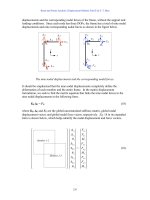
In a steady deceleration phase (ía
x
= constant), the corresponding change in
pitch angle ș
b
can be determined from the equilibrium condition of the additional
horizontal and vertical forces acting at axle distance a, taking into account that the
vertical motion at the axles is ș
b
·a/2 = ǻz (cg at a/2) and
cg x f
hma aV '
which yields
b
ș /2
z
af a  
2
b
ș =[2 /( )]
cg z x b x
hmfa a pa  
(3.25)
The term in brackets is a proportionality factor p
b
between constant linear decel-
eration (ía
x
) and resulting stationary additional pitch angle ș
b

(downward positive
here). The time history of ș after braking control initiation will be constrained by a
second-order differential equation taking into account the effects discussed in con-
nection with Equation 3.24. In visual state estimation to be discussed in Chapter 9,
this knowledge will be taken into account; it is directly exploited in the recursive
estimation process. Figure 3.21 shows, in the top left graph, the pitch rate response
to a step input in acceleration. The softness of the suspension system in combina-
Figure 3.20. Deceleration by braking: Forces, torques,
and orientation change in pitch
+
+
Axle distance a
F
bf
F
b
F
br
Center of gravity cg
h
cg
íș
ǻV
f
í
ǻV
f
í a
x
m·a

x
íI
y
ș
˚˚
additional spring (f
z
·ǻz) and
damper (d ·ǻz) forces
˚
x
Direction of inertial a
x
-measurement
y-direction normal
to the image plane
to the left of driving
direction
z
3.4 Behavioral Capabilities for Locomotion 95
tion with inertia of the body lead to the oscillation extending to almost 2 seconds
after the change in control input. The general second-order dynamic model for an
arbitrary excitation f [a
x
(t)] for braking is given by
22
// [
Sp x
ddtDddtf fat  
TTT

()].
2
(3.26)
Since the eigenfrequency of the vehicle does not change over time and since it is
characteristic of the vehicle in a given loading state, this oscillation over as many
as 50 video cycles can be expected for a certain control input. This alleviates image
sequence interpretation when properly represented in the perception system.
Pitching motion due to partial loss of wheel support: This topic would also fit
under “vertical curvature effects” (above). However, the eigenmotion in pitch after
a step input in wheel support may be understood more easily after the step input in
deceleration has been discussed. Figure 3.22 shows a vehicle that just lost ground
under the front wheels
due to a negative step
input of the supporting
surface while driving at
a certain speed.
The weight (m · g) of the
vehicle together with the
forces at the rear axle
will produce both a
downward acceleration
of the cg and a rotational
acceleration around the
cg. The relations given
at the bottom of the fig-
ure (including D’Alembert inertial forces and moments) yield the differential equa-
tion
222 2
/(/4) /
y

ddta i ga 
T
.
(3.27)
Normalizing the inertial radius i
y
by half the axle distance a/2 to the non-
dimensional inertial radius i
yN
finally yields the initial rotational acceleration
/
dt
Time in seconds
2345678
pitch rate dș/dt
0
d/d
cg - motion above the ground
23 4 5 6 7 8
dz/dt
Road height h step input
Step input of moment M
Y
around
y-axis due to acceleration
Road height h step input
Step input of moment M
Y
around
y-axis due to acceleration

Time in seconds
2345678
2345678
Time in seconds
Time in seconds
0
Figure 3.21. Simulation of vehicle suspension model: Pitch rate (top left) and heave re-
sponse (top right) of ground vehicle suspension after step input in acceleration (center)
as well as the height profile of the ground (bottom)
Figure 3.22. Pitch and downward acceleration after losing
ground contact with the front wheels (cg assumed at cen-
ter of axle distance)
I
y
ș
˚˚
m · g
Center of
gravity cg
§ a/2
+
+
Axle distance a
– mz
˚˚
íF
r
F
r
ș

z §ía/2 ·ș
˚˚
˚˚
F
r
= m · g – m ·z
˚˚
F
r
·a/2 = I
y
ș = m · i
y
²·ș
˚˚
˚˚
3 Subjects and Subject Classes
96
22 2
/2/[(1
yN
ddt ga i  
T
)] .
(3.28)
With i
yN
in the range of 0.8 to 0.9, usually, and axle distances between 2 and
3.5 m for cars, angular accelerations to be expected are in the range from about 6 to
12 rad/s², that is 350 to 700°/s squared resulting in a build–up of angular speed of

about 14 to 28°/s per video cycle time of 40 ms. Inertial sensors will immediately
measure this crisply way, while image interpretation will be confused initially; this
is a strong argument in favor of combined inertial/visual dynamic scene interpreta-
tion. Nature, of course, has discovered these complementarities early and continues
to use them in vertebrate type vision. Figure 3.21 has shown pitch rate and heave
motion after a step input in surface elevation in the opposite direction in the top
two graphs (right-hand part); the response extends over many video cycles (~ 1.5
seconds, i.e., about 35 cycles). Due to tire softness, the effects of a positive or
negative step input will not be exactly the same, but rather similar, especially with
respect to duration.
Pitching and rolling motion due to wheel – ground interaction: A very general
approach to combined visual/inertial perception in ground vehicle guidance would
be to mount linear accelerometers in the vertical direction at each suspension point
of the (four) wheels and additional angular rate sensors around all body axes. The
sum of the linear accelerations measured, integrated over time, would yield heave
motion. Integrals of pairwise sums of accelerometer signals (front vs. rear and left
vs. right-hand side) would indicate pitch and roll accelerations which could then be
fused with the rate sensor data for improved reliability. Their integral would be
available with almost no time delay compared to visual interpretation and could be
of great help when driving in rough terrain, since at least the high-frequency part of
the body orientation would be known for visual interpretation. The (low-
frequency) drift errors of inertial integrals can be removed by results from visual
perception.
Remember the big difference between inertial and visual data interpretation: In-
ertial data are “lead” signals (measured time derivatives) containing the influence
of all kinds of perturbations, while visual interpretation relies very much on models
containing (time-integrated) state variables. In vision, perturbations have to be dis-
covered “in hindsight” when assumptions made do not show up to be valid (after
considerable delay time).
3.4.5.2 Lateral Road Vehicle Guidance

To demonstrate some dynamic effects of details in modeling of the behavior of
road vehicles, the lane change maneuvers with the so-called “bicycle model” (see
Figure 3.10) of a different order are discussed here. First, let us consider an ideal-
ized maneuver (completely decoupled translational motion and no rotations). Ap-
plying a constant lateral acceleration a
y
(of, say, 2 m/s²) in a symmetrical positive
and negative fashion, we look for the time T
LC
in which one lane width W
L
of 3.6
m can be traversed with lateral speed v
y
back to zero again at the end. One obtains
2/
L
CL
TW 
y
a .
(3.29)
3.4 Behavioral Capabilities for Locomotion 97
For the data mentioned, the lane change time is T
LC
= 2.68 seconds, and the
maximum speed at the center of the idealized maneuver is v
ymaxLCi
{t = T
LC

/2} =
2.68 m/s. Since Ackermann steering is nonholonomic, real cars cannot perform this
type of lane change maneuver; however, it is nice as a reference for realizable ma-
neuvers to be discussed in the following. For a
y
= 4 m/s², lane change time would
be 1.9 seconds and maximum lateral speed v
y
(T
LC
/2) = 3.8 m/s.
Fifth-order dynamic model for lateral road vehicle guidance: The very busy
Figure 3.23 shows the basic properties of a simple but full order (linear) bicycle
model, taking combined tire forces from both the left- and right-hand side as well
as translational and rotational dynamics into account. [The full model with all
nonlinearities and separately modeled dynamics for the wheel groups and the body
is too complex to allow analytical solutions; these are used in numerical simula-
tions.] Here, interest lies in some major effects of lateral maneuvering for turns and
lane changes. More involved models may be found in
[Mitschke 1990; Giampiero
2007].
Inertial reference direction
Side forces on the wheels (index y) are generated by introducing an angle of at-
tack at the front wheel(s) through a steering angle Ȝ. Tires may be considered to act
Į
f
Ȝ steer angle (first integral of
control variable)
ȕ side slip angle at cg
yaw rate (inertial)

l
f
distance from cg to front axle
l
r
distance from cg to rear axle
Į
f
angle of attack at front wheel
Į
r
angle of attack at rear wheel
V velocity vector of cg
V
f
velocity vector of front wheel
V
r
velocity vector of rear wheel
P point on longitudinal axis of body
where the velocity vector is
tangential to body
R
r
turn radius of vehicle body
F
ij
tire force components tangential
(index x) and normal to wheel (y)
ȥ

°
l
r
ȥ
°
cg
l
f
ȥ
°
M
M
0
P
l
P
l
r
l
f
R
r
R
r
V
r
V
f
r
ȥ

°
ȕ
V
Axle distance a
¤
f
¤
¤
Ȝ
Į
r
¤
(effective
center of
rotation)
¤
F
xf
F
yf
F
yr
F
xr
ȥ
Ȥ
Figure 3.23. Bicycle model with rotational dynamics
3 Subjects and Subject Classes
98
as springs in the lateral direction with an approximately linear characteristic for

small angles of attack (|Į| < § 3°); only this regime is considered here. For the test
vehicle
VaMoRs, this allows lateral accelerations up to about 0.4 g = 4 m/s² in the
linear range.
With k
T
as the lateral tire force coefficient linking vertical tire force F
N
= m
WL
·g
(wheel load due to gravity) via angle of attack to lateral tire force F
y
, there follows
; .
y
fTfNf yrTrNr
F
kF FkF  
DD
(3.30)
If the vehicle weight is distributed almost equally onto all wheels of a four-
wheel vehicle, m
WL
is close to one quarter of total vehicle mass; in the bicycle
model, it is close to one half the total mass both on the front and rear axle. Defin-
ing the mass related lateral force coefficient k
ltf
/( ) (in m/s²/rad)
ltf y WL f T

kFm kg  
D
,
(3.31)
and multiplying this coefficient with both the actual wheel load (in terms of mass)
and the angle of attack yields the lateral tire force F
y
. The sum of all torques (in-
cluding the inertial D’Alembert-term with I
z
= m · i
z
² as the moment of inertia
around the vertical axis) yields (see Figure 3.23)
(sin cos)
z yr r xf yf
IFlF F lf     

0
\
OO
.
(3.32)
The force balance normal to the vehicle body yields with dȤ/dt = dȤ/ds · ds/dt =
(curvature C of the trajectory driven times speed V), and thus with the centrifugal
force at the cg: C ·V² = m· V· dȤ/dt
/cos /sin
sin cos 0.
yr xf yf
mV d dt md dt

FF F
    
 
F
EE
OO
(3.33)
From the center of Figure 3.23, it can be seen that trajectory heading Ȥ is the
sum of vehicle body heading ȥ and side slip angle ȕ (Ȥ = ȥ + ȕ) and thus
///ddtddtddt. 
F
\E
(3.34)
For small angles of attack at the wheels, the following relations hold after
[Mitschke 1990]:
/ / ; / /
ffr
ddtlV ddtlV    
r
DEO\ DE\
.
(3.35)
For further simplification of the relations, the cg is assumed to lie at the center
between the front and rear axles (l
f
= l
r
= a/2), so that half of the vehicle mass rests
on each axle (wheel of bicycle model: F
Nr

= F
Nf
= mg/2). Then, the following lin-
ear fifth-order dynamic model for lateral control of a vehicle with Ackermann-
steering at constant speed and with the state vector
x
La
(steering angle Ȝ, inertial
yaw rate dȥ/dt, slip angle ȕ, body heading angle ȥ, and lateral position y) results:
T
La
x [ , , , , ]
y


O\E\
.
(3.36)
With the following abbreviations:
22
2
[/(/2)];
/ ; and
/,
zB z
zB ltf
ltf
iia
TVik
TVk



\
E
(3.37)
the set of first-order differential equations is written
3.4 Behavioral Capabilities for Locomotion 99
1
00000
0
/( ) 1/ 0 0 0
0
1/(2 ) 1 1/ 0 0
0
01000
0
00 0
dx d
La
VaT T
d
u
TT
dt
yy
VV
t
§· §·§·
§·

¨¸ ¨¸¨¸
¨¸

¨¸ ¨¸¨¸
¨¸
¨¸ ¨¸¨¸
¨¸


¨¸ ¨¸¨¸
¨¸
¨¸ ¨¸¨¸
¨¸
¨¸
¨¸ ¨¸¨¸
©¹
©¹ ©¹©¹
) 

\\
EE
OO
\\
EE
\\

x bdȜ d.
La
t
(3.38)

For the test vehicle VaMP, a 240 kW (325 HP) powered sedan Mercedes 500
SEL, the parameters involved are (average representative values) m = 2650kg (that
is, m
WL
= m/2 = 1325 kg for the bicycle model), k
T
= 96 kN/rad, I
z
= 5550 kg m²;
and a = 3.14 m. This leads to i
zB
² = 0.85 and k
ltf
§ 72 (m/s² per rad) = 1.25 (m/s² per
degree wheel angle of attack), and finally to the following speed-dependent time
constants for lateral motion (V in m/s):
/84.7 0.01389 ( ) ,
/72 0.0118 ( ).
TV Vs
TV Vs


\
E
(3.39)
These values as a func-
tion of speed V already
have been shown in Figure
3.11 for the test vehicle
VaMP (top right). They in-

crease up to values of 0.9
seconds at maximum
speed. The block diagram
corresponding to Equation
3.38 is shown in Figure
3.24.
From the fact that the
systems dynamics matrix
ĭ has only zeros above the
diagonal and the negative
inverse values of the two time constants on the diagonal, the specialist in systems
dynamics immediately recognizes that the system has three eigenvalues at the ori-
gin of the Laplace-transform “s”-plane (integrators) and two first-order subsystems
with eigenvalues as inverse time constants on the negative real axis; the corre-
sponding time histories are exponentials of the natural number e = 2.71828 of the
form c
i
· exp(ít/T
i
). Since the maximum speed of VaMP is 70 m/s, the eigenvalue
í1/T
ȕ
will range from í to í1 s
í1
. Since amplitudes of first-order systems have
diminished to below 5% in the time range of three time constants, it can be seen
that for speeds above about 1 m/s (§ 3.6 km/h), the dynamic effects should be no-
ticeable in image sequence analysis at video rate (40 ms cycle time). On the other
hand, four video cycles (160 ms) are typical delay times for recognition of complex
scenes by vision including proper reaction so that up to speeds of 4 m/s (§ 14

km/h), neglecting the dynamic effects may be within the noise level (1/T
ȕ3
§ 18
s
í1
).
Figure 3.24. Block diagram of fifth-order (bicycle)
model for lateral control of road vehicles taking rota-
tional dynamics around the vertical axis into account

Ȝ
y
a
V
V
y
°
ȥ
rel
°
ȥ
abs
°


u =
Ȝ
°
ȕ
V

a T
ȥ
ȥ
rel

°
ȕ
C
0h
V

1/T
ȕ
= k
ltf
/
V
k
ltf
/ (2V)
-
-
-
-