Dynamic Vision for Perception and Control of Motion - Ernst D. Dickmanns Part 6 ppt
Bạn đang xem bản rút gọn của tài liệu. Xem và tải ngay bản đầy đủ của tài liệu tại đây (935.91 KB, 30 trang )
5.2 Efficient Extraction of Oriented Edge Features 135
ference is largest in amplitude,
the gradient over two consecu-
tive mask elements is maxi-
mal.
However, due to local per-
turbations, this need not corre-
spond to an actual extreme
gradient on the scale of inter-
est. Experience with images
from natural environments has
shown that two additional pa-
rameters may considerably
improve the results obtained:
1. By allowing a yet to be
specified number n
0
of
entries in the mask center
to be dropped, the results achieved may be more robust. This can be
immediately appreciated when taking into account that either the actual edge
direction may deviate from the mask orientation used or the edge is not
straight but curved; by setting central elements of the mask to zero, the
extreme intensity gradient becomes more pronounced. The rest of Figure 5.10
shows typical mask parameters with n
0
= 1 for masks three and five pixels in
depth (m
d
= 3 or 5), and with n
0
= 2 for m
d
= 8 as well as n
0
= 3 for m
d
= 17
(rows b, c).
2. Local perturbations are suppressed by assigning to the mask a significant
depth n
d
, which designates the number of pixels along the search path in each
row or column in each positive and negative field. The total mask depth m
d
then is m
d
= 2 n
d
+ n
0
. Figure 5.10 shows the corresponding mask schemes. In
line (b) a rather large mask for finding the transition between relatively large
homogeneous areas with ragged boundaries is given (m
d
= 17 pixels wide and
each field with seven elements, so that the correlation value is formed from
large averages; for a mask width n
w
of 17 pixels, the correlation value is
formed from 7·17 = 119 pixels). With the number of zero-values in between
chosen as n
0
= 3, the total receptive field (= mask) size is 17·17 = 289 pixels.
The sum formed from n
d
mask elements (vector values “ColSum”) divided by
(n
w
· n
d
) represents the average intensity value in the oblique image region
adjacent to the edge. At the maximum correlation value found, this is the
average gray value on one side of the edge. This information may be used for
recognizing a specific edge feature in consecutive images or for grouping
edges in a scene context.
For larger mask depths, it is more efficient when shifting the mask along the
search direction, to subtract the last mask element (ColSum-value) from the
summed field intensities and add the next one at the front in the search direction,
see line (c) in Figure 5.10); the number of operations needed is much lower than
for summing all ColSum elements anew in each field.
The optimal value of these additional mask parameters n
d
and n
0
as well as the
mask width n
w
depend on the scene at hand and are considered knowledge gained
Figure 5.10. Efficient mask evaluation with the
“Colsum”-vector; the n
d
-values given are typical
for sizes of “receptive fields” formed
b)
m
d
= 2;
m
d
= 3; m
d
= 5; m
d
= 8
7 3 7
Masks characterized by: (n
d
n
0
n
d
)
m
d
= 17
(Total mask depth)
(a)
(b)
(c)
5 Extraction of Visual Features
136
by experience in visually similar environments. From these considerations, generic
edge extraction mask sets for specific problems have resulted. In Figure 5.11, some
representative receptive fields for different tasks are given. The mask parameters
can be changed from one video frame to the next, allowing easy adaptation to
changing scenes observed continuously, like driving on a curved road.
The large mask in the center top of Figure 5.11 may be used on dirt roads in the
near region with ragged transitions from road to shoulder. For sharp, pronounced
edges like well-kept lane markings, a receptive field like that in the upper right cor-
ner (probably with n
d
= 2, that is, m
d
= 5) will be most efficient. The further one
looks ahead, the more the mask width n
w
should be reduced (9 or 5 pixels); part (c)
in the lower center shows a typical mask for edges on the right-hand side of a
straight road further away (smaller and oblique to the right).
The 5 × 5 (2, 1, 2) mask at the left hand side of Figure 5.11 has been the stan-
dard mask for initial detection of other vehicles and obstacles on the road through
horizontal edges; collections of horizontal edge elements are good indicators for
objects torn by gravity to the road surface. Additional masks are then applied for
checking object hypotheses formed.
If narrow lines like lane markings have to be detected, there is an optimal mask
width depending on the width of the line in the image: If the mask depth n
d
chosen
is too large, the line will be low-pass-filtered and extreme gradients lose in magni-
tude; if mask depth is too small, sensitivity to noise increases.
As an optional step, while adding up pixel values for mask elements “ColSum”
or while forming the receptive fields, the extreme intensity values of pixels in Col-
Sum and of each ColSum vector component (max. and min.) may be determined.
The former gives an indication of the validity of averaging (when the extreme val-
ues are not too far apart), while the latter may be used for automatically adjusting
threshold parameters. In natural environments, in addition, this gives an indication
Figure 5.11. Examples of receptive fields and search paths for efficient edge feature ex-
traction; mask parameters can be changed from one video-frame to the next, allowing
easy adaptation to changing scenes observed continuously
R
e
c
e
p
tiv
e
fie
l
d
o
f
mask
:
n
w
=
1
7
n
=
17
n
w
= 17
Search direction
horizontal
Search path
center
Search direction vertical
(Shift of mask by
1 pixel at a time)
Search path
center (vertical)
Receptive
field of
size 5×5:
n
d
=2; n
0
=1;
edge orien-
tation16
(horizontal)
n
w
= 5
search region
condensed to 1-dimensional
(averaged) vector
n
0
=3
E
d
g
e
o
r
i
e
nt
a
t
i
o
n
5
+
-
0
n
d
=1
E
d
g
e
o
r
i
e
n
t
a
t
i
o
n
5
m
d
= 2·n
d
+ n
0
=14 + 3 = 17
m
d
= 3
For fuzzy large scale edge
For sharp, pro
-
nounced
edge
total = 289 pixel
(tot
al
=
51
p
ix
el)
(a)
(b)
n
w
= 9
Search path
horizontal or
vertical for
diagonal edge
direction
d)
25 pixels
n
0
= 2;
n
w
= 5
Receptive field
total = 30 pixel
(c)
Edge orientation 4
n
d
=7
n
d
=7
+
+
0
-
-
-
+
n
0
=2;
m
d
= 6 :
small base for localizing
edges with larger curvature
++
-
0
0
-
E
d
ge
orientation 8
5.2 Efficient Extraction of Oriented Edge Features 137
of the contrasts in the scene. These are some of the general environmental parame-
ters to be collected in parallel (right-hand part of Figure 5.1).
5.2.2 Search Paths and Subpixel Accuracy
The masks defined in the previous section are applied to rectangular search ranges
to find all possible candidates for an edge in these ranges. The smaller these search
ranges can be kept, the more efficient the overall algorithm is going to be. If the
high-level interpretation via recursive estimation is stable and good information on
the variances is available, the search region for specific features may be confined
to the 3 ı region around the predicted value, which is not very large, usually (ı =
standard variation). It does not make sense first to perform the image processing
part in a large search region fixed in advance and afterwards sort out the features
according to the variance criterion. In order not to destabilize the tracking process,
prediction errors > 3 ı are considered outliers and are usually removed when they
appear for the first time in a sequence.]
Figure 5.6 shows an example of edge localization with a ternary mask of size n
w
= 17, n
d
= 2, and n
0
= 1 (i.e., mask depth m
d
= 5). The mask response is close to
zero when the region to which it is applied is close to homogeneously gray (irre-
spective of the gray value); this is an important design factor for abating sensitivity
to light levels. It means that the plus– and minus regions have to be the same size.
The lower part of the figure shows the resulting correlation values (mask re-
sponses) which form the basis for determining edge location. If the image areas
within each field of the mask are homogeneous, the response is maximal at the lo-
cation of the edge. With different light levels, only the magnitude of the extreme
value changes but not its location. Highly discernible extreme values are obtained
also for neighboring mask orientations. The larger the parameter n
0
, the less pro-
nounced is the extreme value in the search direction, and the more tolerant it is to
deviations in angle. These robustness aspects make the method well suited for
natural outdoor scenes.
Search directions (horizontal or vertical) are automatically chosen depending on
the feature orientation specified. The horizontal search direction is used for mask
orientations between 45 to 135° as well as between 225 and 315°; vertical search is
applied for mask directions between 135 to 225° and 315 to 45°. To avoid too fre-
quent switching between search directions, a hysteresis (dead zone of about one di-
rection–increment for the larger mask widths) is often used that means switching is
actually performed (automatically) 6 to 11° beyond the diagonal lines, depending
on the direction from which these are approached.
5.2.2.1 Subpixel Accuracy by Second-Order Interpolation
Experience with several interpolation schemes, taking up to two correlation values
on each side of the extreme value into account, has shown that the simple second-
order parabola interpolation is the most cost-effective and robust solution (Figure
5.12). Just the neighboring correlation values around a peak serve as a basis.
5 Extraction of Visual Features
138
If an extreme value of the magnitude of
the mask response above the threshold
level (see Figure 5.6) has been found by
stating that the new value is smaller than
the old one, the last three values are used
to find the interpolating parabola of second
order. Its extreme value yields the position
y
extr
of the edge to subpixel accuracy and
the corresponding magnitude C
extr
; this po-
sition is obtained at the location where the
derivative of the parabolic unction is zero.
Designating the largest correlation value
found as C
0
at pixel position 0, the previ-
ous one C
m
at í1, and the last correlation
value C
p
at position +1 (which indicated
that there is an extreme value by its magni-
tude C
p
< C
0
), the following differences
00m 1m
= ; = DCC DCC
p
(5.1)
yield the location of the extreme value at distance
01
extr 0
extr 0 1
d 0.5/ (2 / 1)
from pixel position 0, such that: y = y + d
with the value = 0.25 d .
y DD
y
CC Dy
(5.2)
From the last expressions of Equation 5.1 and 5.2 it is seen that the interpolated
value lies on the side of C
0
on which the neighboring correlation value measured is
larger. Experience with real-world scenes has shown that subpixel accuracy in the
range of 0.3 to 0.1 may be achieved.
5.2.2.2 Position and Direction of an Optimal Edge
Determining precise edge direction by applying, additionally, the two neighboring
mask orientations in the same search path and performing a bi–variant interpola-
tion has been investigated, but the
results were rather disappointing.
Precise edge direction can be de-
termined more reliably by exploit-
ing results from three neighboring
search paths with the same mask
direction (see Figure 5.13).
The central edge position to
subpixel accuracy yields the posi-
tion of the tangent point, while the
tangent direction is determined
from the straight line connecting
the positions of the (equidistant)
neighboring edge points; this is
Figure 5.13. Determination of the tangent di-
rection of a slightly curved edge by sub-pixel
localization of edge points in three neighboring
search paths and parabolic interpolation
Figure 5.12. Subpixel edge localiza-
tion by parabolic interpolation after
passing a maximum in mask response
5.2 Efficient Extraction of Oriented Edge Features 139
the result of a parabolic interpolation for the three points.
Once it is known that the edge is curved – because the edge point at the center
does not lie on the straight line connecting the neighboring edge points – the ques-
tion arises whether the amount of curvature can also be determined with little effort
(at least approximately). This is the case.
5.2.2.3 Approximate Determination of Edge Curvature
When applying a series of equidistant search stripes to an image region, the method
of the previous section yields to each point on the edge also the corresponding edge
direction that is its tangent. Two points and two slopes determine the coefficients
of a third-order polynomial, dubbed Hermite-interpolation after a French mathema-
tician. As a third-order curve, it can have at most one inflection point. Taking the
connecting line (dash-dotted in Figure 5.14) between the two tangent points P
-d
and
P
+d
as reference (chord line or secant), a simple linear relationship for a smooth
curve with small angles ȥ relative to the chord line can be derived. Tangent direc-
tions are used in differential-geometry terms, yielding a linear curvature model; the
reference is the slope of the straight line connecting the tangent points (secant). Let
m
íd
and m
+d
be the slopes of the tangents at points P
íd
and P
+d
respectively; s be the
running variable in the direction of the arc (edge line); and ȥ the angle between the
local tangent and the chord direction (|ȥ| < 0.2 radian so that cos(ȥ) §1).
The linear curvature model in differential-geometry terms with s as running
variable along the arc s from x §íd to x § +d is:
0 1
+ ; dȥ dCCCs Cs
1
Cs
.
(5.3)
Since curvature is a second-order concept with respect to Cartesian coordinates,
lateral position y results from a second integral of the curvature model. With the
origin at the center of the chord, x in the direction of the chord, y normal to it, and
ȥ
íd
= arctan(m
-d
) § m
íd
as the angle between the tangent and chord directions at
point P
íd
, the equation describing the curved arc then is given by Equation 5.4 be-
low [with ȥ in the range ± 0.2 radian (~ 11°), the cosine can be approximated by 1
and the sine by the argument ȥ]:
0001
0
23
0000
0
x = + ; ȥ(s) ȥ + (ı) dıȥ+ /2 ;
y(s) = + sin[ȥ(ı)] dı ȥ /2 /6.
s
2
s
ds C Cs+Cs
yysCs
³
³
(5.4)
At the tangent points at the ends of the chord (± d), there is
2
dd00 1
2
+d +d 0 0 1
ȥ = ȥ + /2; (a)
ȥ = ȥ + + /2. (b)
mCdCd
mCdCd
|
|
(5.5)
At the points of intersection of chord and curve, there is, by definition y(± d) = 0,
23
00 0 1
23
00 0 1
() ȥ /2 /6 0; (a)
() ȥ /2 /6 0. (b)
yd y dCd Cd
yd y dCd Cd
(5.6)
Equations 5.5 and 5.6 can be solved for the curvature parameters C
0
and C
1
as
well as for the state values y
0
and m
0
(ȥ
0
) at the origin x = 0 to yield
5 Extraction of Visual Features
140
0
2
1
0
0
( )/(2 ),
1.5 ( )/ ,
ȥ 0.25 ( ),
0.25 ( ) .
dd
dd
dd
dd
Cmm d
Cmmd
mm
ymmd
(5.7)
The linear curva-
ture model can be
computed easily from
the tangent directions
relative to the chord
line and the distance
(2·d) between the
tangent points. Of
course, this distance
has to be chosen such
that the angle con-
straint (|ȥ| < 0.2 ra-
dian) is not violated.
On smooth curves,
this is always possi-
ble; however, for
large curvatures, the distance d allowed becomes small and the scale for measuring
edge locations and tangent directions probably has to be adapted. Very sharp
curves have to be isolated and jumped over as “corners” having large directional
changes over small arc lengths. In an idealized but simple scheme, they can be ap-
proximated by a Dirac impulse in curvature with a finite change in direction over
zero arc length.
Due to the differencing process unavoidable for curvature determination, the re-
sults tend to be noisy. When basic properties of objects recognized are known, a
post–processing step for noise reduction exploiting this knowledge should be in-
cluded.
Remark: The special advantage of subscale resolution for dynamic vision lies in
the fact that the onset of changes in motion behavior may be detected earlier, yield-
ing better tracking performance, crucial for some applications. The aperture prob-
lem inherent in edge tracking will be revisited in Section 9.5 after the basic track-
ing problem has been discussed.
5.2.3 Edge Candidate Selection
Usually, due to image noise there are many insignificant extreme values in the re-
sulting correlation vector, as can be seen in Figure 5.6. Positioning the threshold
properly (and selecting the mask parameters in general) depends very much on the
scene at hand, as may be seen in Figure 5.15, due to shadow boundaries and scene
noise, the largest gradient values may not be those looked for in the task context
(road boundary). Colinearity conditions (or even edge elements on a smoothly
Figure 5.14. Approximate determination of curvature of a
slightly curved edge by sub-pixel localization of edge points
and tangent directions: Hermite-interpolation of a third order
parabola from two tangent points
P
-d
P
+d
m
-d
m
+d
y
0
= 0.25 (m
+d
– m
íd
)
d
Linear curvature model:
C = C
0
+ C
1
· s; í d < s < + d
·d
s
C
0
= (m
+d
– m
íd
)/(2·d)
C
1
= 1.5·(m
-d
+ m
+d
)/d
2
Ȍ
íd
= arctan(m
íd
) § m
íd
Ȍ
-d
íd
0
y
x
Ȍ
0
= í 0.25·(m
íd
+ m
+d
)
0
5.2 Efficient Extraction of Oriented Edge Features 141
Figure 5.15. The challenge of edge feature selection in road scenes: Good decisions can
be made only by resorting to higher level knowledge. Road scenes with shadows (and
texture); extreme correlation values marking road boundaries may not be the absolutely
largest ones.
curved line) may be needed for proper feature selection; therefore, threshold selec-
tion in the feature extraction step should not eliminate these candidates. Depending
on the situation, these parameters have to be specified by the user (now) or by a
knowledge-based component on the higher system levels of a more mature version.
Average intensity levels and intensity ranges resulting from region-based methods
(see Section 5.3) will yield information for the latter case.
As a service to the user, in the code
CRONOS, the extreme values found in one
function call may be listed according to their correlation values; the user can spec-
ify how many candidates he wants presented at most in the function call. As an ex-
treme value of the search either the pixel position with the largest mask response
may be chosen (simplest case with large measurement noise), or several neighbor-
ing correspondence values may be taken into account allowing interpolation.
5.2.4 Template Scaling as a Function of the Overall “Gestalt”
An additional degree of freedom available to the designer of a vision system is the
focal length of the camera for scaling the image size of an object to its distance in
the scene. To analyze as many details as possible of an object of interest, one tends
to assume that a focal length, which lets the object (in its largest dimension) just
fill the image would be optimal. This may be the case for a static scene being ob-
served from a stationary camera. If either the object observed or the vehicle carry-
5 Extraction of Visual Features
142
ing the camera or both can move, there should be some room left for searching and
tracking over time. Generously granting an additional space of the actual size of
the object to each side results in the requirement that perspective mapping (focal
length) should be adjusted so that the major object dimension in the image is about
one third of the image. This leaves some regions in the image for recognizing the
environment of the object, which again may be useful in a task context.
To discover essential shape details of an object, the smallest edge element tem-
plate should not be larger than about one-tenth of the largest object dimension.
This yields the requirement that the size of an object in the image to be analyzed in
some detail should be about 20 to 30 pixels. However, due to the poor angular
resolution of masks with a size of three pixels, a factor of 2 (60 pixels) seems more
comfortable. This leads to the requirement that objects in an image must be larger
than about 150 pixels. Keep in mind that objects imaged with a size (region) of
only about a half dozen pixels still can be noticed (discovered and roughly
tracked), however, due to spurious details from discrete mapping (rectangular pixel
size) into the sensor array, no meaningful shape analysis can be performed.
This has been a heuristic discussion of the effects of object size on shape recog-
nition. A more operational consideration based on straight edge template matching
and coordinate-free differential geometry shape representation by piecewise func-
tions with linear curvature models is to follow.
A lower limit to the support region required for achieving accuracy of about
one-tenth of a pixel in a tangent position and about 1° in the tangent direction (or-
der of magnitude) by subpixel resolution is about eight to ten pixels. The efficient
scheme given in
[Dickmanns 1985] for accurately determining the curvature parame-
ters is limited to a smooth change in the tangent direction of about 20 to 25°; for
recovering a circle (360°). This means that about n
elef
§ 15 to 18 elemental edge
features have to be measured. Since the ratio of circumference to diameter is ʌ for
a circle, the smallest circle satisfying these conditions for non–overlapping support
regions is n
elef
times (mask size = 8 to 10 pixels) divided by ʌ. This yields a re-
quired size of about 40 to 60 pixels in linear extension of an object in an image.
Since corners (points of finite direction change) can be included as curvature
impulses measurable by adjacent tangent directions, the smallest (horizontally
aligned) measurable square is ten pixels wide while the diagonal is about 14 pixels;
more irregularly shaped objects with concavities require a larger number of tangent
measurements. The convex hull and its dimensions give the smallest size measur-
able in units of the support region. Fine internal structures may be lost.
From these considerations, for accurate shape analysis down to the percent
range, the image of the object should be between 20 and 100 pixel in linear exten-
sion, in general. This fits well in the template size range from 3 (or 5) to 17 (or 33)
pixels. Usual image sizes of several hundred lines allow the presence of several
well-recognizable objects in each image; other scales of resolution may require dif-
ferent focal lengths for imaging (from microscopy to far ranging telescopes).
Template scaling for line detection: Finally, choosing the right scale for detecting
(thin) lines will be discussed using a real example
[Hofmann 2004]. Figure 5.16
shows results for an obliquely imaged lane marking which appears 16 pixels wide
in the search direction (top: image section searched, width n
w
= 9 pixel). Summing
up the mask elements in the edge direction corresponds to rectifying the image
5.2 Efficient Extraction of Oriented Edge Features 143
stripe, as shown below in the figure; however, only one intensity value remains, so
that for the rest of the pixel-operations with different mask sizes in the search di-
rection, about one order of magnitude in efficiency is gained. All five masks inves-
tigated (a) to (e) rely on the same “ColSum”-vector; depending on the depth of the
masks, the valid search ranges are reduced (see double-arrows at bottom).
Figure 5.16. Optimal mask size for line recognition: For general scaling, mask size
should be scaled by line width (= 16 pixels here)
The averaged intensity profile of the mask elements is given in the vertical cen-
ter (around 90 for the road, and ~130 for the lane marker); the lane marking clearly
sticks out. Curve (e) shows the mask response for the mask of highest possible
resolution (1, 0, 1); see legend. It can be seen that the edge is correctly detected
with respect to location, but due to the smaller extreme value, sensitivity to noise is
higher than that for the other masks. All other masks have been chosen with n
0
= 3
for reducing sensitivity to slightly different edge directions including curved edges.
In practical terms, this means that the three central values under the mask shifted
over the ColSum–vector need not be touched; only n
d
values to the left and to the
right need be summed.
Depth values for the two fields of the mask of n
d
= 4, 8, and 16 (curves a, b, c)
yield the same gradient values and edge location; the mask response widens with
increasing field width. By scaling the field depth n
d
of the mask by the width of the
line l
w
to be detected, the curves can be generalized to scaled masks of depths n
d
/l
w
= ¼, ½, and 1. Case (d) shows with n
d
/l
w
= 21/16 = 1.3 that for field depths larger
than line width, the maximal gradient decreases and the edge is localized at a
wrong position. So, the field width selected should always be smaller than the line
to be detected. The number of zeros at the center should be less than the field
depth, probably less than half that value for larger masks; values between 1 and 3
have shown good results for n
d
up to 7. For the detection of dirt roads with jagged
edges and homogeneous intensity values on and off the road, large n
0
are favorable.
5 Extraction of Visual Features
144
5.3 The Unified Blob-edge-corner Method (UBM)
The approach discussed above for detecting edge features of single (sub-) objects
based on receptive fields (masks) has been generalized to a feature extraction
method for characterizing image regions and general image properties by oriented
edges, homogeneously shaded areas, and nonhomogeneous areas with corners and
texture. For characterizing textures by their statistical properties of image intensi-
ties in real time (certain types of textures), more computing power is needed; this
has to be added in the future. In an even more general approach, stripe directions
could be defined in any orientation, and color could be added as a new feature
space. For efficiency reasons, here, only horizontal and vertical stripes in intensity
images are considered, for which only one matrix index and the gray values vary at
a time). To achieve reusability of intermediate results, stripe widths are confined to
even numbers and are decomposed into two half-stripes.
5.3.1 Segmentation of Stripes through Corners, Edges, and Blobs
In this image evaluation method, the goal is to start from as few assumptions on in-
tensity distributions as possible. Since pixel noise is an important factor in outdoor
environments, some kind of smoothing has to be taken into account, however. This
is done by fitting models with planar intensity distribution to local pixel values if
they exhibit some smoothness conditions; otherwise, the region will be character-
ized as nonhomogeneous. Surprisingly, it has turned out that the planarity check
for local intensity distribution itself constitutes a nice feature for region segmenta-
tion.
5.3.1.1 Stripe Selection and Decomposition into Elementary Blocks
The field size for the least-squares fit of a planar pixel-intensity model is (2·m) ×
(2·n), and is called the “model support region” or mask region. For reusability of
intermediate results in computation, this support region is subdivided into basic
(elementary) image regions (called mask elements or briefly “mels”) that can be
defined by two numbers: The number of pixels in the row direction m, and the
number of pixels in the column direction n. In Figure 5.17, m has been selected as
4 and n as 2; the total stripe width for row search thus is 4 pixels. For m = n = 1,
the highest possible image resolution will be obtained; however, strong influence
of noise on the pixel level may show up in the results in this case.
When working with video fields (sub–images with only odd or even row–
indices, as is often done in practical applications), it makes sense for horizontal
stripes to choose m = 2n; this yields averaging of pixels at least in row direction for
n = 1. Rendering these mels as squares, finally yields the original rectangular im-
age shape with half the original full-frame resolution. By shifting stripe evaluation
by only half the stripe width, all intermediate pixel results in one half-stripe can be
reused directly in the next stripe by just changing sign (see below). The price to be
paid for this convenience is that the results obtained have to be represented at the
5.3 The Unified Blob-edge-corner Method (UBM) 145
center point of the support region which is exactly at pixel boundaries. However,
since subpixel accuracy is looked for anyway, this is of no concern.
Figure 5.17. Stripe definition (row = horizontal, column = vertical) for the (multiple)
feature extractor ‘UBM’ in a pixel-grid; mask elements (mels) are defined as basic rec-
tangular units for fitting a planar intensity model
Values in these half-stripes of stripe 2 are stored for reuse in stripe 3
1
Half-
stripe
Stripe ‘C2’
Stripe ‘C1’
Stripe ‘C3’
Center points of
mel regions
Stripe ‘C4’
1 2 3 4 5 Number of half-
stripe
Image region
evaluated
n = 2
m = 4
No gradient direction in this
mask: region marked as
non–homogeneous
mel
y, u
z, v
Right Left
R L
in se arch
direc tion
column (C)
Center of mask
Stored newly
com-
puted
1half-
stripe
Stripe
‘R2’
Stripe
‘R1’
Stripe
‘R3’
Edge direction
Center points of
mel regions
Image region
evaluated: mask
Left L
Right
R
in search
direction row (R)
Gradient direction
Number of
half-stripe
1
2
3
4
5
6
.
Rows are evaluated top-down;
columns from left to right.
Still open is the question of how to proceed within a stripe. Figure 5.17 suggests
taking steps equal to the width of mels; this covers all pixels in the stripe direction
once and is very efficient. However, shifting mels by just 1 pixel in the stripe di-
rection yields smoother (low-
pass filtered) results
[Hofmann
2004]. For larger mel-lengths, in-
termediate computational results
can be used as shown in Figure
5.18.
This corresponds to the use of
Colsum in the method CRONOS
(see Figures 5.9 and 5.10). The
new summed value for the next
mel can be obtained by subtract-
ing the value of the last column
and adding the one of the next
Figure 5.18. Mask elements (mels) for efficient
computation of gradients and average intensities
-
+
+
-
+
-
cell at position ‘j’
cell at position ‘j+1’
‘j-2’
‘j+2’
‘j’
horizontal
gradient
vertical
gradient
resulting
cell structure
incremental computation of cell values for cells
with larger extension in stripe direction
Step
1
5 Extraction of Visual Features
146
column [(jí2) and (j+2) in the example shown, bottom row in Figure 5.18].
For the vertical search direction, image evaluation progresses top-down within
the stripe and from left to right in the sequence of stripes. Shifting of stripes is al-
ways done by mel-size m or n (width of half-stripe), while shifting of masks in the
search direction can be specified from 1 to m or n (see Figure 5.19b below); the lat-
ter number m or n means pure block evaluation, however, only coarse resolution.
This yields the lowest possible computational load with all pixels used just once in
one mel. For objects in the near range, this may still be sufficient for tracking.
The goal was to obtain an algorithm allowing easy adaptation to limited com-
puting power; since high resolution is required in only a relatively small part of
images, in general in outdoor scenes, only this region needs to be treated with more
finely tuned parameters (see Figure 5.37 below). Specifying a rectangular region of
special interest by its upper left and lower right corners, this sub-area can be pre-
cisely evaluated in a separate step. If no view stabilization is available, the decision
for the corner points may even be based on actual evaluation results with coarse
resolution. The initial analysis with coarse resolution guarantees that only the most
promising subregions of the image are selected despite angular perturbations
stemming from motion of the subject body, which shifts around the inertially fixed
scene in the image. This attention-focusing avoids unnecessary details in regions of
less concern.
Figure 5.19 shows the definitions necessary for performing efficient multiple-
scale feature evaluation. The left part (a) shows the specification of masks of dif-
ferent sizes (with mel-sizes from 1×1 to 4×2 and 4×4, i.e., two pyramid stages).
Note that the center of a pixel or of mels does not coincide with the origin O of the
masks, which is for all masks at (0, 0). The mask origin is always defined as the
point where all four quadrants (mels) meet. The computation of the average inten-
Figure 5.19. With the reference points chosen here for the mask and the average image
intensities in quadrants Qi, fusing results from different scales becomes simple; (a) basic
definitions of mask elements, (b) progressive image analysis within stripes and with se-
quences of stripes (shown here for rows)
Ɓ
Mask in stripe R
ií1
at index k–1
Mask in stripe R
i
at index k
Center
of pixel (1, 1)
in (mel in Q4
with average
mel–intensity I
22
)
0
= origin of mask
-4 -3 -2 -1 0 1 2 3 4
-4
-3
-2
-1
0
1
2
3
4
Mask with mask element mel = 4×4
Mask with mask elements 3 × 3
Mask with
mask elements 2×2
mel = 1×1
mask element
4 × 2
Position
(0.5, 0.5)
y, m
u
z v
n
Row
Col-
umn
Q1
=
I
12
Q2
=
I
11
Q3
=
I
21
Q4
=
I
22
Mel-centers
4×2
4×4
3×3
Mask in stripe R
i+1
at index k+1
(b)
(
a
)
•
•
•
•
•
•
Mask 4×4
mel = 2×2
i
5.3 The Unified Blob-edge-corner Method (UBM) 147
sities in each mel (I
12
, I
11
, I
21
, I
22
in quadrants Q1 to Q4) is performed with the ref-
erence point at (0.5, 0.5), the center of the first pixel nearest to the mask origin in
the most recent mel; this yields a constant offset for all mask sizes when rendering
pixel intensities from symbolic representations. For computing gradients, of
course, the real mel centers shown in quadrant Q4 have to be used.
The reconstruction of image intensities from results of one stripe is done for the
central part of the mask (± half the size of the width normal to the search direction
of the mask element). This is shown in the right part (b) of the figure by different
shading. It shows (low-frequency) shifting of the stripe position by n = 2 (index i)
and (high-frequency) shifting of the mask position in search direction by 1 (index
k). Following this strategy in both row and column direction will yield nice low-
pass-filtered results for the corresponding edges.
5.3.1.2 Reduction of the Pixel Stripe to a Vector with Attributes
The first step is to sum up all n pixel or cell values in the direction of the width of
the half-stripe (lower part in Figure 5.18). This reduces the half-stripe for search to
a vector, irrespective of stripe width specified. It is represented in Figure 5.18 by
the bottom row (note the reduction in size at the boundaries). Each and every fur-
ther computation is based on these values that represent the average pixel or cell
intensity at the location in the stripe if divided by the number of pixels summed.
However, these individual divisions are superfluous computations and can be
spared; only the final results have to be scaled properly for image intensity.
In our example with m = 4 in Figure 5.18, the first mel value has to be computed
by summing up the first four values in the vector. When the mels are shifted by one
pixel or cell length for smooth evaluation of image intensities in the stripe (center
row), the four new mel values are obtained by subtracting the trailing pixel or cell
value at position j í2 and by adding the leading one at j +2 (see lower left in Figure
5.18). The operations to be performed for gradient computation in horizontal and
vertical directions are shown in the upper left and center parts of the figure. Sum-
ming two mel values (vertically in the left and horizontally in the center sub-
figure) and subtracting the corresponding other two sums yields the difference in
(average) intensities in the horizontal and vertical directions of the support region.
Dividing these numbers by the distances between the centers of the mels yields a
measure of the (averaged) horizontal and vertical image intensity gradient at that
location. Combining both results allows computing the absolute gradient direction
and magnitude. This corresponds to determining a local plane tangent to the image
intensity distribution for each support region (mask) selected.
However, it may not be meaningful to enforce a planar approximation if the in-
tensities vary irregularly by a large amount. For example, the intensity distribution
in the mask top left of Figure 5.17 shows a situation where averaging does not
make sense. Figure 5.20a shows the situation with intensities as vectors above the
center of each mel. For simplicity, the vectors have been chosen of equal magni-
tude on the diagonals. The interpolating plane is indicated by the dotted lines; its
origin is located at the top of the central vector representing the average intensity
I
C
. From the dots at the center of each mel in this plane, it can be recognized that
two diagonally adjacent vectors of average mel intensity are well above, respec-
5 Extraction of Visual Features
148
tively, below the interpolating
plane. This is typical for two cor-
ners or a textured area (e.g., four
checkerboard fields or a saddle
point).
Figure 5.20b represents a per-
fect (gray value) corner. Of
course, the quadrant with the dif-
fering gray value may be located
anywhere in the mask. In general,
all gray values will differ from
each other. The challenge is to
find algorithms allowing reason-
able separation of these feature
types versus regions fit for inter-
polation with planar shading models (lower part of Figure 5.20) at low computa-
tional cost. Well known for corner detection among many others are the “Harris”-
[Harris, Stephens 1988], the KLT- [Tomasi, Kanade 1991] and the “Haralick”-
[Haralick, Shapiro 1993] algorithms, all based on combinations of intensity gradients
in several regions and directions. The basic ideas have been adapted and integrated
into the algorithm UBM. The goal is to segment the image stripe into regions with
smooth shading, corner points, and extended nonhomogeneous regions (textured
areas). It will turn out that nonplanarity is a new, easily computable feature on its
own (see Section 5.3.2.1).
Figure 5.20. Feature types detectable by UBM
in stripe analysis
Corner points are of special value in tracking since they often allow determining
optical feature flow in image sequences (if robustly recognizable); this is one im-
portant hint for detecting moving objects before they have been identified on
higher system levels. These types of features have shown good performance for de-
tecting pedestrians or bicyclists in the near range of a car in urban traffic
[Franke et
al. 2005]
.
Stripe regions fit for approximation by sequences of shading models are charac-
terized by their average intensities and their intensity gradients over certain regions
in the stripe; Figure 5.20c shows such a case. However, it has to be kept in mind
that a planar fit to intensity profiles with nonlinear intensity changes in only one di-
rection can yield residues of magnitude zero with the four symmetric support
points in the method chosen (see Figure 5.20d); this is due to the fact that three
points define a plane in space, and the fourth point (just one above the minimal
number required for fixing a plane) is not sufficient for checking the real spatial
structure of the surface to be approximated. This has to be achieved by combining
results from a sequence of mask evaluations.
By interpolation of results from neighboring masks, extreme values of gradients
including their orientation are determined to subpixel accuracy. Note that, contrary
to the method
CRONOS, no direction has to be specified in advance; the direction
of the maximal gradient is a result of the interpolation process. For this reason the
method UBM is called “direction-sensitive” (instead of “direction selective” in the
case of
CRONOS). It is, therefore, well suited for initial (strictly “bottom-up”) im-
age analysis
[Hofmann 2004], while CRONOS is very efficient once predominant
5.3 The Unified Blob-edge-corner Method (UBM) 149
edge directions in the image are known and their changes can be estimated by the
4-D approach (see Chapter 6).
During these computations within stripes, some statistical properties of the im-
ages can be determined. In step 1, all pixel values are compared to the lowest and
the highest values encountered up to then. If one of them exceeds the actual ex-
treme value, the actual extreme is updated. At the end of the stripe, this yields the
maximal (I
max-st
) and the minimal (I
min-st
) image intensity values in the stripe. The
same statistic can be run for the summed intensities normal to the stripe direction
(I
wmax-st
and I
wmin-st
) and for each mel (I
cmax-st
and I
cmin-st
); dividing the maximal and
minimal value within each mel by the average for the mel, these scaled values will
allow monitoring the appropriateness of averaging. A reasonable balance between
computing statistical data and fast performance has to be found for each set of
problems.
Table 5.1 summarizes the parameters for feature evaluation in the algorithm
UBM; they are needed for categorizing the symbolic descriptions within a stripe,
for selecting candidates, and for merging across stripe boundaries. Detailed mean-
ings will be discussed in the following sections.
Table 5.1. Parameters for feature evaluation in image stripes
ErrMax Maximally allowed percent error of interpolated intensity
plane through centers of four mels (typically 3 to 10%);
note that the errors at all mel centers have same magnitude!
(see Section 5.3.2.2)
CircMin
(qmin)
Minimal “circularity” required, threshold value on scaled
second eigenvalue for corner selection [0.75 corresponds to
an ideal corner (Figure 5.20b), the maximal value 1 to an
ideal double–corner (checkerboard, Figure 5.20a)]; (see
section 5.3.3)
traceNmin (Alternate) threshold value for selection of corner candi-
dates; useful for adjusting the number of corner candidates.
IntensGradMin Threshold value for intensity gradients to be accepted as
edge candidates; (see Section 5.3.2.3)
AngleFactHor Factor for limiting edge directions to be found in horizontal
search direction (rows); (see Section 5.3.2.3)
AngleFactVer Factor for limiting edge directions to be found in vertical
search direction (columns); (see Section 5.3.2.3)
VarLim Upper bound on variance allowed for a fit on both ends of
a linearly shaded blob segment
Lsegmin Minimum length required of a linearly shaded blob seg-
ment to be accepted (suppression of small regions)
DelIthreshMerg Tolerance in intensity for merging adjacent regions to 2-D
blobs
DelSlopeThrsh Tolerance for intensity gradients for merging adjacent re-
gions to 2-D blobs
The five feature types treated with the method UBM are (1) textured regions
(see Section 5.3.2.1), (2) edges from extreme values of gradients in the search di-
rection (see Section 5.3.2.3), (3) homogeneous segments with planar shading mod-
5 Extraction of Visual Features
150
els (see Section 5.3.2.4), (4) corners (see Section 5.3.3), and (5) regions nonline-
arly shaded in one direction, which, however, will not be investigated further here.
They have to lie between edges and homogeneously shaded areas and may be
merged with class 1 above.
The sequence of decisions in the unified approach to all these features, exploit-
ing the same set of image data evaluated in a stripe-wise fashion, is visualized in
Figure 5.21. Both horizontal and vertical stripes may be searched depending on the
orientation of edges in the image. Localization of edges is best if they are oriented
close to orthogonal to the search direction; therefore, for detecting horizontal edges
and horizontal blob boundaries, a vertical search should be preferred. In the general
case, both search directions are needed, but edge detection can then be limited to
(orthogonal to the search direction) ± 50°. The advantage of the method lies in the
fact that (1) the same feature parameters derived from image regions are used
throughout, and (2) the regions for certain features are mutually exclusive. Com-
pared to investigating the image separately for each feature type, this reduces the
computer workload considerably.
Figure 5.21. Decision tree for feature detection in the unified blob-edge-corner method
(UBM) by local and global gradients in the mask region
Bi-directional nonplanarity
check via ratio R of difference
over sum of intensities on
diagonals: ErrMax > R ?
I
11
I
12
I
21
I
22
no
yes
Store in list of
‘nonlinearly shaded’
segments
Update description of
candidates for homo-
geneous shading
yes
yes
no
Are the conditions
for corner candidates
satisfied? (circularity > q
min
)
‘and’ (traceN > traceN
min
)
Store in list of
corner
candidates
Store in list of inhomogeneous
segments (texture)
D1 = I
11
+ I
22
D2 = I
12
+ I
21
Dif = D1íD2
Sm= D1+D2
R = Dif / Sm
Check conditions for an
extreme value of intensity
gradient: product [(last d.o.g.)
×(actual d.o.g.*)] < 0]?
mask
*d.o.g.=
difference of gradients
Determine edge location and edge
orientation to subpixel accuracy;
store in list of ‘edge features’
At the end of each stripe,
Select
‘best local’
corner points
(local q
max
)
Search for the best local
linearly shaded intensity regions (blobs);
(Variance at boundaries < VarLim)
‘and’ (segment length > Lseg
min
)
Compare results with previous stripe and merge regions
of similar shading (intensity and gradient components);
this yields 2-D homogeneously shaded blobs.
5.3 The Unified Blob-edge-corner Method (UBM) 151
5.3.2 Fitting an Intensity Plane in a Mask Region
For more efficient extraction of features with respect to computing time, as a first
step the sum of pixel intensities I
cs
is formed within rectangular regions, so-called
cells of size m
c
× n
c
; this is a transition to a coarser scale. For m
c
= n
c
, pyramid lev-
els are computed, especially for m
c
= n
c
= 2 the often used step-2 pyramids. With I
ij
as pixel intensity at location u = i and v = j there follows for the cell
11
.
cc
mn
cs ij
ij
I
I
¦¦
(5.8)
The average intensity
c
I of all pixels in the cell region then is
/( ).
ccscc
IImn
(5.9)
The normalized pixel intensity I
pN
for each pixel in the cell region is
/
p
Npc
I
II around the average value
c
I
.
(5.10)
Cells of different sizes may be used to generate multiple scale images of reduced
size and resolution for efficient search of features on a larger scale. When working
with video fields, cells of size 2 in the row and 1 in the column direction will bring
some smoothing in the row direction and lead to much shorter image evaluation
times. When coarse-scale results are sufficient, as for example with high-resolution
images for regions nearby, cells of size 4 × 2 efficiently yield scene characteristics
for these regions, while for regions further away, full resolution can be applied in
much reduced image areas; this foveal–peripheral differentiation contributes to ef-
ficiency in image sequence evaluation. The region of high-resolution image
evaluation may be directed by an attention focusing process on a higher system
level based on results from a first coarse analysis (in a present or previous image).
The second step is building mask elements (“mels”) from cells; they contain
pixels in the search direction, and
pixels normal to the search direction.
cp
cp
mm m
nn n
(5.11)
Define
,
11
mn
MEs cs ij
ij
I
I
¦¦
(sum of cell intensities)
CS
I
,
(5.12)
then the average intensity of cells and thus also of pixels in the mask element is
/( )
ME MEs
IImn .
(5.13)
In the algorithm UBM, mels are the basic units on which efficiency rests. Four
of those are always used to form masks (see Figures 5.17-5.19) as support regions
for image intensity description by symbolic terms:
Masks are support regions for the description and approximation of local
image intensity distributions by parameterized symbols (image features):
(1) ‘Textured areas’ (nonplanar elements), (2), ‘oriented edges’ (3) ‘linearly
shaded regions’, and (4) ‘corners’. Masks consist of four mask elements
(mels) with average image intensities
11 12 21 22
,,,
s
sss
I
III.
5 Extraction of Visual Features
152
The average intensity of all mels in the mask region is
,11122122
()
Mean s s s s s
I IIII /4.
(5.14)
To obtain intensity elements of the order of magnitude 1, the normalized inten-
sity in mels is formed by division by the mean value of the mask:
,
/.
ijN ijs Mean s
III
(5.15)
This means that
/4 1.
ijN
I
ªº
¬¼
¦
(5.16)
The (normalized) gradient components in a mask then are given as the differ-
ence of intensities divided by the distance between mel-centers:
1N
r 12N 11N
f=I I m (upper row direction) (a)
2
22 21
-
N
rNN
fII m (lower row direction) (b)
1
21 11
N
cNN
fII n (left column direction) (c)
2
22 12
-
N
cNN
fII n (right column direction). (d)
(5.17)
The first two are local gradients in the row-direction (index r) and the last two in
the column direction (index c). The global gradient components of the mask are
12
2
NNN
rrr
fff (global row direction)
12
2
NNN
ccc
fff (global column direction).
(5.18)
The normalized global gradient g
N
and its angular orientation ȥ then are
22
NN
N
rc
g
ff
(5.19)
ȥ arctan /
NN
cr
ff .
(5.20)
ȥ is the gradient direction in the (u, v)-plane. The direction of the vector normal to
the tangent plane of the intensity function (measured from the vertical) is given by
arctan
N
Ȗ g .
(5.21)
5.3.2.1 Adaptation of a Planar Shading Model to the Mask Area
The origin of the local coordinate system used is chosen at the center of the mask
area where all four mels meet. The model of the planar intensity approximation
with least sum of the squared errors in the four mel–centers has the yet unknown
parameters I
0
, g
y
, and g
z
(intensity at the origin, and gradients in the y- and z-
directions). According to this linear model, the intensities at the mel–centers are
11 0
12 0
21 0
22 0
/2 /2,
/2 /2,
/2 /2,
/2 /2.
Np y z
Np y z
Np y z
Np y z
IIgmgn
IIgmgn
IIgmgn
IIgmgn
(5.22)
Let the measured values from the image be
11 12 21
,,
N
NN
III
PPP
and
22
N
I
P
. Then the er-
rors e
ij
can be written:
5.3 The Unified Blob-edge-corner Method (UBM) 153
11 11 11
11
0
12 12 12
12
21 21 21
21
22 22 22
22
1/2/2
1/2/2
1/2/2
1/2/2
Np N N
Np N N
y
Np N N
z
Np N N
II I
e
mn
I
II I
e
mn
g
II I
e
mn
g
II I
e
mn
PP
PP
PP
PP
ª
º
ªº
ªº
ªº
«
»
«»
«»
«»
«
»
«»
«»
«»
«
»
«»
«»
«»
«
»
«»
«»
¬¼
¬¼
¬¼
¬
¼
.
(5.23)
To minimize the sum of the squared errors, this is written in matrix form:
N
eAgI
P
(a)
where (b)
1111
/2 /2 /2 /2
/2 /2 /2 /2
T
Amm mm
nnnn
ªº
«
«
«»
¬¼
»
»
(5.24)
and . (c)
11 12 21 22
T
NNNNN
IIIII
P PPPP
ªº
¬¼
The sum of the squared errors is and shall be minimized by proper selection
of
T
ee
0
T
yz
I
g g p
ªº
¬¼
. The necessary condition for an extreme value is that the par-
tial derivative ; this leads to
()/ 0
T
dee dp
TT
N
A
IAA
P
p ,
(5.25)
with solution (pseudo–inverse)
1
()
TT
N
pAAAI
P
.
(5.26)
From Equation 5.24b follows
2
2
40 0
00
00
T
AA m
n
ª
º
«
»
«
»
«
»
¬
¼
and
12
2
1/4 0 0
() 01/ 0
001/
T
AA m
n
ªº
«»
«»
«»
¬¼
,
(5.27)
and with Equations 5.24c and 5.14
12
12
2
2
4
/2
/2
NN
NN
T
Nrr
cc
AI f f m
ffn
P
ª
º
«
»
«
»
«
»
«
»
¬
¼
.
(5.28)
Inserting this into Equation 5.26 yields, with Equation 5.17, the solution
0
[ ]= [1 ].
T
yz rN cN
pIgg ff
(5.29)
5.3.2.2 Recognizing Textured Regions (limit for planar approximations)
By substituting Equation 5.29 into 5.23, forming
12 11
()ee
and
22 21
(ee)
as well
as and , and by summing and differencing the results, one fi-
nally obtains
21 11
()ee
22 12
(ee )
21 12
ee
(5.30)
5 Extraction of Visual Features
154
and
11 22
ee ;
this means that the errors on each diagonal are equal. Summing up all errors
yields, with Equation 5.16,
ij
e
0
ij
e
¦
.
This means that the errors on the diagonals have opposite signs, but their magni-
tudes are equal! These results allow an efficient combination of feature extraction
algorithms by forming the four local gradients after Equation 5.17 and the two
components of the gradient within the mask after Equations 5.18 and 5.29. All four
errors of a planar shading model can thus be determined by just one of the four
Equations 5.23. Even better, inserting proper expressions for the terms in Equation
5.23, the planar interpolation error with Equation 5.12 turns out to be
11 22 12 21 MEs
ErrInterp[()()]/
I
IIII .
(5.31)
Efficiently programmed, its evaluation requires just one additional difference
and one ratio computation. The planar shading model is used only when the magni-
tude of the residues is sufficiently small
p
l,max
| ErrInterp | H
(dubbed ErrMax).
(5.32)
MaxErr = 4%; 1291 features in row–, 2859 in column search
0.59% of pixels 1.3% of pixels
Figure 5.22. Nonplanarity features in central rectangle of an original video–field
(cell size m
c
= 1, n
c
= 1, mel size 1×1, finest possible resolution, MaxErr = 4%)
Figure 5.22 shows a video field of size 288 × 768 pixels with nonplanar regions
for m
c
= n
c
= m = n =1 (highest possible resolution) and ErrMax = 4% marked by
white dots; regions at the left and right image boundaries as well as on the motor
hood (lower part) and in the sky have been excluded from evaluation.
Only the odd or even rows of a full video frame form a field; fields are transmit-
ted every 40 ms in 25 Hz video. Confining evaluation to the most interesting parts
of fields leaves the time of the complementary field (20 ms) as additional comput-
ing time; the image resolution lost in the vertical direction is hardly felt with sub-
pixel feature extraction. [Interleaved video frames (from two fields) have the addi-
tional disadvantage that for higher angular turn rates in the row direction while
taking the video, lateral shifts result between the fields.]
The figure shows that not only corner regions but also – due to digitization ef-
fects – some but not all edges with certain orientations (lane markings on the left
and parts of silhouettes of cars) are detected as nonplanar. The number of features
detected strongly depends on the threshold value ErrMax.
5.3 The Unified Blob-edge-corner Method (UBM) 155
Figure 5.23 shows a
summary of results for the
absolute number of masks
with nonplanar intensity
distribution as a function
of a variety of cell and
mask parameters as well
as of the threshold value
ErrMax in percent. If this
threshold is selected too
small (say, 1%), very
many nonplanar regions
are found. The largest
number of over 35 000 is
obtained if a mask element
is selected as a single
pixel; this corresponds to
~ 17% of all masks evalu-
ated of the image.
The number of nonpla-
nar regions comes down
rapidly for higher values
of ErrMax. For ErrMax =
2%, this number drops to
less than 1/3; for higher
values of ErrMax, the
scale has been changed in
the figure for better resolution. For ErrMax = 5%, the maximum number of non-
planar masks is less than 2000, that is less than 1% of the number of original pix-
els; on the other hand, for all cell and mask parameters investigated in the range [1
(m
c
, n
c
) 2 and 1 (m, n) 4], the number of nonplanar intensity regions does
not drop below ~ 600 (for ErrMax = 5%). This is an indication that there is signifi-
cant nonplanarity in intensity distribution over the image which can be picked up
by any set of cell and mask parameters and also by the computer-efficient ones
with higher parameter values that show up in the lower curves of Figure 5.23. Note
that these curves include working on the first pyramid level m
c
= n
c
= 2 with mask
elements m 4 and n 4; only the lowest curve 11.44 (m = n =1, m
c
= n
c
= 4), for
which the second pyramid level has been formed by preprocessing during cell
computation, shows ~ 450 nonplanar regions for ErrMax = 5%. The results point in
the direction that a combination of features from different pyramid scales will form
a stable set of features for corner candidates.
For the former set of parameters (first pyramid level), decreasing the threshold
value ErrMax to 3% leaves at least ~ 1500 nonplanar features; for curve 11.44, to
reach that number of nonplanar features, ErrMax has to be lowered to 2%; how-
ever, this corresponds to ~ 50 % of all cell locations in this case. Averaging over
cells or mask elements tends to level-off local nonplanar intensity distributions; it
may therefore be advisable to lower threshold ErrMax in these cases in order not to
Figure 5.23. Absolute number of mask locations with
residues exceeding ErrMax for a wide variety of cell
and mask parameters m, n, m
c
, n
c
. For ErrMax 3% a
new scale is used for better resolution. For ErrMax
5% at most 2000 nonplanar intensity regions are found
out of at most ~ 200 000 mask locations for highest
resolution with mel = pixel in a video–field.
1 2 3 4 5 6 7 8
0
5
10
15
20
25
30
35
ErrMax %
Absolute number of occurrences (thousands)
11.11
0
0.5
1
1.5
2
2.5
3
3.5
4
4.5
11.44
Absolute number of locations
of nonplanarity
5 Extraction of Visual Features
156
lose sharp corners of moderate intensity differences. On the contrary, one might
guess that for high resolution images, analyzed with small parameter values for
cells and masks, it would be advantageous to increase ErrMax to get rid of edges
but to retain corners. To visualize the 5%-threshold, Figure 5.24 shows the video
field with intensities increased within seven rectangular regions by 2, 3, 4, 5, 7.5,
10, and 15% respectively; the manipulation is hardly visible in darker regions for
values less than 5%, indicating that this seems to be a reasonable value for the
threshold ErrMax from a human observer’s point of view. However, in brighter
image regions (e.g., sky), even 3% is very noticeable.
The effect of lifting the threshold value ErrMax to 7.5% for planar intensity ap-
proximation for highest resolution (all parameters = 1, in shorthand notation
(11.11) for the sequel) is shown in Figure 5.25.
In comparison to Figure 5.22, it can be seen that beside many edge positions
many corner candidates have also been lost, for example, on tires and on the dark
truck in front. This indicates that to keep candidates for real corners in the scene,
ErrMax should not be chosen too large. The threshold has to be adapted to the
scene conditions treated. There is not yet sufficient experience available to auto-
mate this threshold adaptation which should certainly be done based on results
ErrMax =
2 % 3 % 4 % 5 % 7.5 % 10 %
15 %
Figure 5.24. Visualization of %–threshold values in image intensity for separating pla-
nar from nonplanar local intensity models: In the rectangles, all pixel values have been
increased by a factor corresponding to the percentage indicated as inset
Figure 5.25. Nonplanar features superimposed on original videofield for the threshold
values MaxErr = 4% (left) and 7.5% (right); cell size m
c
= 1, n
c
= 1, mel size 1×1 (rows
compressed after processing). More than 60% of features are lost in right image.
5.3 The Unified Blob-edge-corner Method (UBM) 157
from several sets of parameters (m
c
, n
c
, m, n) and with a payoff function yet to be
defined. Values in the range 2 ErrMax 5% are recommended as default for re-
ducing computer load, on the one hand, and for keeping good candidates for cor-
ners, on the other.
Larger values for mel and cell parameters should be coupled with smaller values
of ErrMax. Working on the first (2×2) pyramid level of pixels (cell size m
c
= 2, n
c
= 2) reduces the number of mask evaluations needed by a factor of 8 compared to
working on the pixel level. The third power of 2 is due to the fact that now the
half-stripe in the number of pixels is twice as wide as in the number of cells; in to-
tal, this is roughly a reduction of one power of 10 in computing effort (if the pyra-
mid image is computed simultaneously with frame grabbing by a special device).
Figure 5.26 shows a juxtaposition of results on the pixel level (left) and on the
first pyramid level (right). For ErrMax = 2% on the pixel level (left part), the 4% of
occurrences of the number of nonplanar regions corresponds to about 8000 loca-
tions, while on the first pyramid level,
16% corresponds to about 4000 locations
(see reference numbers on the vertical scale). Thus, the absolute number of non-
planar elements decreases by about a factor of 2 on the first pyramid level while
the relative frequency in the
image increases by about a
factor of 4. Keeping in
mind that the number of
image elements on the first
pyramid level has de-
creased by the same factor
of 4, this tells us that on this
level, most nonplanar fea-
tures are preserved. On the
pixel level, many spurious
details cause the frequency
of this feature to increase;
this is especially true if the
threshold ErrMax is re-
duced (see leftmost ordi-
nate in Figure 5.26 for
ErrMax = 1%).
For the largest part of
standard images from
roads, therefore, working on the first pyramid level with reduced resolution is suf-
ficient; only for the farther look-ahead regions on the road, which appear in a rela-
tively small rectangle around the center, is full resolution recommended. Quite
naturally, this yields a foveal–peripheral differentiation of image sequence analysis
with much reduced computing resources needed. Figure 5.27 demonstrates that
when working with video fields, a further reduction by a factor of 2 is possible
without sacrificing detection of significant nonplanar features.
The right-hand picture is based on cell size (4×2); 4 pixels each in two rows are
summed to yield cell intensity, while on the left, the cell is a pixel on the (2×2) first
pyramid level. The subfigures are superpositions of all pixels found to belong to
Figure 5.26. Relative number of nonplanar mask lo-
cations as a function of parameters for mask element
formation m, n, m
c
, n
c
. Note that in the right part
ErrMax starts at 2%; in the left part, which represents
working on the pixel level, the relative frequency of
nonplanar regions is down to ~ 4% for this value.
Threshold ‘ErrMax’ in % of average intensity value
1 2 3 4 5
18
16
14
12
10
8
6
4
2
0
occurrence in % of ~ 200 000
mask locations (pixels)
Number of
mask locations
with nonplanar
intensity distri-
bution for vari-
ous m, n and
m
c
= n
c
= 1
2 3 4 5
18
16
14
12
10
8
6
4
2
0
Number of mask
locations with
nonplanar cell
intensity distribu-
tion for various
m, n and
m
c
= n
c
= 2
occurrence in % of ~ 25 000
mask locations (cells)
5 Extraction of Visual Features
158
Figure 5.27. Nonplanar features for parameter set ErrMax = 2.5%, mask elements m =
n = 2 and cell size n
c
= m
c
= 2 (i.e., first pyramid level, left; after processing compressed
2:1 in rows for better comparison). Changing m
c
to 4 (right) yields about the same num-
ber of features : ~ 2500.
nonplanar regions, both in row search (horizontal white bars) and in column search
(vertical white bars); it can be seen that beside corner candidates many edge candi-
dates are also found in both images. For similar appearance to the viewer, the left
picture has been horizontally compressed after finishing all image processing.
From the larger number of local vertical white bars on the left, it can be seen that
nonplanarity still has a relatively large spread on the first pyramid level; the larger
cell size of the right-hand image cuts the number of masks to be analyzed in half
(compare results in corner detection in Figure 5.39, 5.40 below). Note that even the
reflections on the motor hood are detected. The locations of the features on differ-
ent scales remain almost the same. These are the regions where stable corner fea-
tures for tracking can be found, avoiding the aperture problem (sliding along
edges). All significant corners for tracking are among the nonplanar features. They
can now be searched for with more involved methods, which however, have to be
applied to candidate image regions at least an order of magnitude smaller (see Fig-
ure 5.26). After finding these regions of interest on a larger scale first, for precise
localization full resolution may be applied in those regions.
5.3.2.3 Edges from Extreme Values of Gradients in Search Direction
Gradient values of the intensity
function have to be determined
for least-squares fit of a tangent
plane in a rectangular support re-
gion (Equation 5.29). Edges are
defined by extreme values of the
gradient function in the search
direction (see Figure 5.28). These
can easily be detected by multi-
plying two consecutive values of
their differences in the search di-
rection [(g
0
í g
m
)·(g
p
í g
0
)]; if the
sign of the product is negative,
an extreme value has been
í1 0 +1
i í 2 i í 1 i
Mask location for evaluation
g
m
g
extr
y
extr
y
dy
D0
-D1
g
p
< g
0
g
0
g
extr
g
m
g
p
(a)
(b)
Intensity
gradient
g
Int
intensity
Threshold
parameters:
• IntGradMin
• EpsGradCurv
í1
0.
Figure 5.28. Localization of an edge to subpixel
accuracy by parabolic interpolation after passing
a maximum value g
0
of the intensity gradient
5.3 The Unified Blob-edge-corner Method (UBM) 159
passed. Exploiting the same procedure shown in Figure 5.12, the location of the ex-
treme value can be determined to sub-cell accuracy. This indicates that accuracy is
not necessarily lost when cell sizes are larger than single pixels; if the signals are
smooth (and they become smoother by averaging over cells), the locations of the
extreme values may be determined to better than one-tenth the cell size. Mel sizes
of several pixels in length and width (especially in the search direction), therefore,
are good candidates for efficient and fast determination of edge locations with this
gradient method.
Figure 5.28a shows three gradient values g
m
, g
0
, and g
p
determining the parabola
to be interpolated. The second-order coefficient of this parabolic curve, dubbed
“mintcurv” is given by
0
mintcurv 0.5 ( ) -
mp
g
gg .
(5.33)
To eliminate noise effects from data, two threshold values are introduced before an
edge is computed:
1. The magnitude of mintcurv has to be larger than a threshold value İ
intcurv
; this
eliminates very shallow extremes (large radii of the osculating circles, dashed
lines in 5.28a). Leaving this threshold out may often be acceptable.
2. The absolute value of the maximum gradient encountered has to be larger than a
threshold value “IntGradMin”; this admits only significant gradients as candi-
dates for edges. The larger the mel size, the smaller this threshold should be
chosen.
Proper threshold values for classes of problems have to be found by experimenta-
tion; in the long run, the system should be capable of doing this by itself, given
corresponding payoff functions.
Since edges oriented directly in
the search direction are prone to
larger errors, they can be ex-
cluded by limiting the ratio of
the gradient components for ac-
ceptance of candidates. Figure
5.29 shows the principal idea.
When both gradient compo-
nents |g
y
| and |g
z
| are equal, the
edge direction is 45°. Excluding
all cases where Equation 5.34 is
valid, a selection of k
Į
around 1
will allow finding all edges by a
combined row and column
search.
,
|| ||
y
hor z
g
k
D
!g
|
in row search and
|| |
,
z
vert y
g
kg
D
!
Figure 5.29. Limiting edge directions to be found
in row–search around the vertical can be achieved
by introducing limits for the ratio of gradient
components (|g
y
| / |g
z
| > k
Į,hor
); (analogous for col-
umn search: k
Į,hor
need not be equal to k
Į,vert
)
in column search ,
(5.34)
(Edges with orientation close to diagonal should be detected in both search direc-
tions, leading to redundancy for cross checking.) Sub-mel localization of edges is
performed only when all conditions mentioned are satisfied. The extreme value is
found where the derivative of the gradient is zero. Defining
g
y
g
z1
g
z2
= g
y
g
y
/ k
Į,hort
= g
z3
45°
Setting the
exclusion factor
k
Į
= 0.8 and
requesting
|g
y
| > k
Į,hor
·|g
z
| ,
edge directions in
the range ± ~ 50 °
(case 3) from the
orthogonal to the
search direction
are picked up.
Edge
directions
case 1
case 3
case 2