Dynamic Vision for Perception and Control of Motion - Ernst D. Dickmanns Part 7 pptx
Bạn đang xem bản rút gọn của tài liệu. Xem và tải ngay bản đầy đủ của tài liệu tại đây (550.66 KB, 30 trang )
5.3 The Unified Blob-edge-corner Method (UBM) 165
L
segmin
= 4 pyramid-pixels or 16 original image pixels. Figure 5.35 shows the re-
sults for column search (top left), for row search (top right), and superimposed re-
sults, where pixels missing in one reconstructed image have been added from the
other one, if available.
The number of blobs to be handled is at least one order of magnitude smaller
than for the full representation underlying Figure 5.34. For a human observer, rec-
ognizing the road scene is not difficult despite the pixels missing. Since homoge-
neous regions in road scenes tend to be more extended horizontally, the superposi-
tion ‘column over row’ (bottom right) yields the more naturally looking results.
Note, however, that up to now no merging of blob results from one stripe to the
next has been done by the program. When humans look at a scene, they cannot but
do this unwillingly and apparently without special effort. For example, nobody will
have trouble recognizing the road by its almost homogeneously shaded gray val-
ues. The transition from 1-D blobs in separate stripes to 2-D blobs in the image and
to a 3-D surface in the outside world are the next steps of interpretation in machine
vision.
5.3.2.5 Extended Shading Models in Image Regions
The 1-D blob results from stripe analysis are stored in a list for each stripe, and are
accumulated over the entire image. Each blob is characterized by
1. the image coordinates of its starting point (row respectively column num-
ber and its position j
ref
in it),
2. its extension L
seg
in search direction,
3. the average intensity I
c
at its center, and
4. the average gradient components of the intensity a
u
and a
v
.
This allows easy merging of results of two neighboring stripes. Figure 5.36a shows
the start of 1-D blob merging when the threshold conditions for merger are satis-
fied in the region of overlap in adjacent stripes: (1) The amount of overlap should
exceed a lower bound, say, two
or three pixels. (2) The differ-
ence in image intensity at the
center of overlap should be
small. Since the 1-D blobs are
given by their cg-position (u
bi
= j
ref
+ L
seg,i
/2), their ‘weights’
(proportional to the segment
length L
seg,i
), and their intensity
gradients, the intensities at the
center of overlap can be com-
puted in both stripes (I
covl1
) and
I
covl2
) from the distance be-
tween the blob center and the
center of overlap exploiting the
gradient information. This
yields the condition for accep-
tance
•
•
Ž
cg
2
cg
1
L
seg1
= 12
L
seg2
= 6
Figure 5.36. Merging of overlapping 1-D blobs in
adjacent stripes to a 2-D blob when intensity and
gradient components match within threshold limits
cg
S
įu
cg
įv
cg
u
b1
u
v
įu
S
2
įv
S2
(a) Merging of first two 1-D blobs to a 2-D blob
(b) Recursive merging of a 2-D blob with an overlap-
ping 1-D blob to an extended 2-D blob.
įu
S3
Ž
cg
Snew
S
2D
= L
seg1
+ L
seg2
= 18
•
L
seg3
= 6
cg
3
įv
cg
cg
2D
= cg
Sold
•
įv
S3
5 Extraction of Visual Features
166
cov 1 cov 2
||
ll
I
I DelIthreshMerg .
(5.37)
Condition (3) for merging is that the intensity gradients should also lie within small
common bounds (difference < DelSlopeThrsh, see Table 5.1).
If these conditions are all satisfied, the position of the new cg after merger is
computed from a balance of moments on the line connecting the cg’s of the regions
to be merged; the new cg of the combined areas S
2D
thus has to lie on this line. This
yields the equation (see Figure 5.36a)
12
()
S seg cg S seg
įuL įu įuL 0,
(5.38)
and, solved for the shift įu
S
with S
2D
= L
seg1
+ L
seg2
, the relation
21 2 22
/( ) /
S seg seg seg cg cg seg D
įuL L L įu įuL S
(5.39)
is obtained. The same is true for the v-component
21 2 22
/( ) / .
S seg seg seg cg cg seg D
įvL L L įv įvL S
(5.40)
Figure 5.36b shows the same procedure for merging an existing 2-D blob, given
by its weight S
2D
, the cg-position at cg
2D
, and the segment boundaries in the last
stripe. To have easy access to the latter data, the last stripe is kept in memory for
one additional stripe evaluation loop even after the merger to 2-D blobs has been
finished. The equations for the shift in cg are identical to those above if L
seg1
is re-
placed by S
2Dold
. The case shown in Figure 5.36b demonstrates that the position of
the cg is not necessarily inside the 2-D blob region.
A 2-D blob is finished when in the new stripe no area of overlap is found any
more. The size S
2D
of the 2-D blob is finally given by the sum of the L
seg
-values of
all stripes merged. The contour of the 2-D blob is given by the concatenated lower
and upper bounds of the 1-D blobs merged. Minimum (u
min
, v
min
) and maximum
values (u
max
, v
max
) of the coordinates yield the encasing box of area
encbox max min max min
= ( ) ( ).Auuvv (a)
(5.41)
A measure of the compactness of a blob is the ratio
compBlob 2 encbox
/
D
RSA . (b)
For close to rectangular shapes it is close to 1; for circles it is ʌ/4, for a triangle it is
0.5, and for an oblique wide line it tends toward 0. The 2-D position of the blob is
given by the coordinates of its center of gravity u
cg
and v
cg
. This robust feature
makes highly visible blobs attractive for tracking.
5.3.2.6 Image Analysis on two Scales
Since coarse resolution may be sufficient for the near range and the sky, fine scale
image analysis can be confined to that part of the image containing regions further
away. After the road has been identified nearby, the boundaries of these image re-
gions can be described easily around the subject’s lane as looking like a “pencil
tip” (possibly bent). Figure 5.37 shows results demonstrating that with highest
resolution (within the white rectangles), almost no image details are lost both for
the horizontal (left) and the vertical search (right).
The size and position of the white rectangle can be adjusted according to the ac-
tual situation, depending on the scene content analyzed by higher system levels.
Conveniently, the upper left and lower right corners need to be given to define the
5.3 The Unified Blob-edge-corner Method (UBM) 167
Reconstructed image (horizontal):
Coarse (4x4)
Fine
Coarse resolution
Reconstructed image (vertical):
Coarse (4x4)
Fine
Coarse resolution
Figure 5.37. Foveal–peripheral differentiation of image analysis shown by the ‘imag-
ined scene’ reconstructed from symbolic representations on different scales: Outer
part 44.11, inner part 11.11 from video fields compressed 2:1 after processing; left:
horizontal search, right: vertical search, with the Hofmann operator.
rectangle; the region of high resolution should be symmetrical around the horizon
and around the center of the subject’s lane at the look-ahead distance of interest, in
general.
5.3.3 The Corner Detection Algorithm
Many different types of nonlinearities may occur on different scales. For a long
time, so-called 2-D-features have been studied that allow avoiding the “aperture
problem”; this problem occurs for features that are well defined only in one of the
two degrees of freedom, like edges (sliding along the edge). Since general texture
analysis requires significantly more computing power not yet available for real-
time applications in the general case right now, we will also concentrate on those
points of interest which allow reliable recognition and computation of feature flow
[Moravec 1979; Harris, Stephens 1988; Tomasi, Kanade 1991; Haralick, Shapiro 1993].
5.3.3.1 Background for Corner Detection
Based on the references just mentioned, the following algorithm for corner detec-
tion fitting into the mask scheme for planar approximation of the intensity function
has been derived and proven efficient. The structural matrix
22
11 12
12
22
21 22
12
( )2
2( )
rN rN rN cN
rN cN c N c N
nn
ff ff
N
nn
ff f f
§·
§·
¨
¨¸
©¹
©¹
¸
(5.42)
has been defined with the terms from Equations 5.17 and 5.18. Note that compared
to the terms used by previously named authors, the entries on the main diagonal are
formed from local gradients (in and between half-stripes), while those on the cross-
diagonal are twice the product of the gradient components of the mask (average of
the local values). With Equation 5.18, this corresponds to half the sum of all four
cross-products
5 Extraction of Visual Features
168
12 21
,1,2
0.5 ( )
riN cjN
ij
nn ff
¦
.
(5.43)
This selection yields proper tuning to separate corners from planar elements in
all possible cases (see below). The determinant of the matrix is
2
11 22 12
det -wNnnn
.
(5.44)
With the equations mentioned, this becomes
11 22
1112 2212 1212
det 0.75
0.5 ( ) .
cc rr rr cc
Nnn
nff nff ffff
(5.45)
Haralick calls the “Beaudet measure of cornerness”, however,
formed with a different term
det Nw
12 ri ci
n ff 6 . The eigenvalues O of the structural
matrix are obtained from
11 12
2
11 22 12
12 22
0,
nn
nnn
nn
O
ªº
O O
«»
O
¬¼
22
11 22 11 22 12
0nn n n nO O .
(5.46)
With the quadratic enhancement term Q,
11 22
2Qnn ,
(5.47)
there follows for the two eigenvalues
12
,OO,
2
1,2
11detQNQ
ªº
O r
¬¼
.
(5.48)
Normalizing these with the larger eigenvalue
1
O
yields
1N 2N 2 1
1 ; /O O OO;
2
2
1 1 det / 1 1 det /
N
NQ NQO
2
.
(5.49)
Haralick defines a measure of circularity q as
2
12 12
2
12
12
4
1q
ªº
OO OO
«»
OO
OO
¬¼
.
(5.50)
With Equation 5.48 this reduces to
22
11 22 12 11 22
det / 4 ( )/( )qNQ nnnnn
2
,
(5.51)
and in normalized terms (see Equation 5.49), there follows
2
2N 2N
= 4 Ȝ / (1 + Ȝ ).q
(5.52)
It can thus be seen that the normalized second eigenvalue Ȝ
2N
and circularity q
are different expressions for the same property. In both terms, the absolute magni-
tudes of the eigenvalues are lost.
Threshold values for corner points are chosen as lower limits for the determi-
nant detN = w and circularity q:
min
ww!
and
min
qq! .
(5.53)
In a post-processing step, within a user-defined window, only the maximal value
of w = w* is selected.
5.3 The Unified Blob-edge-corner Method (UBM) 169
Harris was the first to use the eigenvalues of the structural matrix for threshold
definition. For each location in the image, he defined the performance value
2
(,) det ( )
H
Ryz N trace N D
,
(5.54)
where
12
det N O O and
12
2trace N Q O O ,
(5.55)
yielding
2
12 1 2
H
R OO D O O
º
¼
. (a)
(5.56)
With ( , see Equation 5.49), there follows
21
/N O O
2N
O
2
2
1
1
H
R
ª
O ND N
¬
. (b)
For R
H
0 and 0 ț 1, D has to be selected in the range,
2
0 ț / 1 0.25dDd N d .
(5.57)
Corner candidates are points for which R
H
0 is valid; larger values of D yield
fewer corners and vice versa. Values around D = 0.04 to 0.06 are recommended.
This condition on R
H
is equivalent to (from Equations 5.44, 5.53, and 5.54)
2
det 4NQ!D .
(5.58)
Kanade et al. (1991) (KLT) use the following corner criterion: After a smooth-
ing step, the gradients are computed over the region D·D (2 d D d 10 pixels). The
reference frame for the structural matrix is rotated so that the larger eigenvalue O
1
points in the direction of the steepest gradient in the region
22
1
K
LT r c
ffO .
(5.59)
O
1
is thus normal to a possible edge direction. A corner is assumed to exist if O
2
is sufficiently large (above a threshold value O
2thr
). From the relation det N = O
1
· O
2
,
the corresponding value of O
2KLT
can be determined
21
det
K
LT KLT
NO O.
(5.60)
If
2KLT 2thr
O!O,
(5.61)
the corresponding image point is put in a candidate list. At the end, this list is
sorted in decreasing order of O
2KLT
, and all points in the neighborhood with smaller
O
2KLT
values are deleted. The threshold value has to be derived from a histogram of
O
2
by experience in the domain. For larger D, the corners tend to move away from
the correct position.
5.3.3.2 Specific Items in Connection with Local Planar Intensity Models
Let us first have a look at the meaning of the threshold terms circularity (q in Equa-
tion 5.50) and trace N (Equation 5.55) as well as the normalized second eigenvalue
(Ȝ
2N
in Equation 5.49) for the specific case of four symmetrical regions in a 2 × 2
mask, as given in Figure 5.20. Let the perfect rectangular corner in intensity distri-
bution as in Figure 5.38b be given by local gradients f
r1
= f
c1
= 0 and f
r2
= f
c2
= íK.
Then the global gradient components are f
r
= f
c
= íK/2. The determinant Equation
5 Extraction of Visual Features
170
5.44 then has the value det N = 3/4·K
4
. The term Q (Equation 5.47) becomes Q =
K
2
, and the “circularity” q according to Equation 5.51 is
2
det / = 4/3 = 0. 75.qNQ
(5.62)
The two eigenvalues of the structure matrix are Ȝ
1
= 1.5·K
2
, and Ȝ
2
= 0.5·K
2
so
that traceN = 2Q is 4·
K
2
; this yields the normalized second eigenvalue as Ȝ
2N
= 1/3.
Table 5.2 contains this case as the second row. Other special cases according to the
intensity distributions given in Figure 5.38 are also shown. The maximum circular-
ity of 1 occurs for the checkerboard corners in Figure 5.38a and row 1 in Table 5.2;
the normalized second eigenvalue also assumes its maximal value of 1 in this case.
The case Figure 5.38c (third row in the table) shows the more general situation
with three different intensity levels in the mask region. Here, circularity is still
close to 1 and Ȝ
2N
is above 0.8. The case in Figure 5.38e with constant average
mask intensity in the stripe is shown in row 5 of Table 5.2: Circularity is rather
high at q = 8/9 § 0.89 and Ȝ
2N
= 0.5. Note that from the intensity and gradient val-
ues of the whole mask this feature can only be detected by g
z
(I
M
and g
y
) remain
constant along the search path.
By setting the minimum required circularity q
min
as the threshold value for ac-
ceptance to
min
0.7q ,
(5.63)
Figure 5.38. Local intensity gradients on mel-level for calculation of circularity q in
corner selection: (a) Ideal checker-board corner: q = 1. (b) ideal single corner: q = 0.75;
(c) slightly more general case (three intensity levels, closer to planar); (d) ideal shading,
one direction only (linear case for interpolation, q § 0); (e) demanding (idealized) corner
feature for extraction (see text).
f
r2
= 0
f
c2
f
r1
= 0
f
c1
(a)
(b)
f
r1
= 0
f
r1
f
c1
f
r2
f
c2
f
c2
f
r2
f
c1
(c)
f
r2
f
f
r1
= 0
f
c1
c
(e)
(d)
I
12
=1
I
22
=0
I
21
=0.5
I
11
=0.5
I
mean
= 0.5
row
y
column
z
f
r2
= í 0.5
f
r1
= 0.5
f
c1
= 0
f
c2
= í1
g
y
= 0
g
z
= í0.5 = g
g
z
= g = 0
g
y
= 0
g
z
= g =
í1
Shifting location of
evaluation mask
5.3 The Unified Blob-edge-corner Method (UBM) 171
all significant cases of intensity corners will be picked. Figure 5.38d shows an al-
most planar intensity surface with gradients –K in the column direction and a very
small gradient ± İ in the row direction (K >> İ). In this case all characteristic val-
ues: det N, circularity q, and the normalized second eigenvalue Ȝ
2N
all go to zero
(row 4 in the table). The last case in Table 5.2 shows the special planar intensity
distribution with the same value for all local and global gradients (–K); this corre-
sponds to Fig 5.20c. It can be seen that circularity and Ȝ
2N
are zero; this nice fea-
ture for the general planar case is achieved through the factor 2 on the cross-
diagonal of the structure matrix Equation 5.42.
When too many corner candidates are found, it is possible to reduce their number
not by lifting q
min
but by introducing another threshold value traceN
min
that limits
the sum of the two eigenvalues. According to the main diagonals of Equations 5.42
and 5.46, this means prescribing a minimal value for the sum of the squares of all
local gradients in the mask.
Table 5.2. Some special cases for demonstrating the characteristic values of the structure
matrix in corner selection as a function of a single gradient value K. TraceN is twice the va-
lue of Q (column 4).
Example Local gradi-
ent values
Det. N
Equation
5.44
Term Q
Equation
5.47
Circula-
rity q
Ȝ
1
Ȝ
2N
=
Ȝ
2/
Ȝ
1
Figure
5.38a
+, – K (2 each) 4 K
4
2 K
2
12K
2
1
Figure
5.38b
0, – K (2 each) ¾ K
4
K
2
0. 75 1.5 K
2
0.3333
Figure
5.38c
0, –K (f
c1
, f
r2
),
–2K
5 K
4
3 K
2
5/9
= 0.556
5 K
2
0.2
Figure
5.38e
f
ri
= ± K
f
ci
= 0; – 2K
8 K
4
3 K
2
8/9 4 K
2
0.5
Figure
5.38d
f
ri
= ±İ (<< K)
f
ci
= – K
4 * İ
2
K
2
§ 0
(İ
2
+K
2
)
§ K
2
~ 4 İ
2
/K
2
§ 0
§ 2 *
(K
2
- İ
2
)
§ 2İ
2
/K
2
§ 0
Planar f
i,j
= – K (4×) 0 2 K
2
04 * K
2
0
This parameter depends on the absolute magnitude of the gradients and has thus to
be adapted to the actual situation at hand. It is interesting to note that the planarity
check (on 2-D curvatures in the intensity space) for interpolating a tangent plane to
the actual intensity data has a similar effect as a low boundary of the threshold
value, traceN
min
.
5.3.4 Examples of Road Scenes
Figure 5.39 left shows the nonplanar regions found in horizontal search (white
bars) with ErrMax = 3%. Of these, only those locations marked by cyan crosses
have been found satisfying the corner condition q
min
= 0.6 and traceN
min
= 0.11.
The figure on the right-hand side shows results with the same parameters except
the reduction of the threshold value to traceN
min
= 0.09, which leaves an increased
5 Extraction of Visual Features
172
Figure 5.39. Corner candidates derived from regions with planar interpolation resi-
dues > 3% (white bars) with parameters (m, n, m
c
, n
c
= 3321). The circularity threshold
q
min
= 0.6 eliminates most of the candidates stemming from digitized edges (like lane
markings). The number of corner candidates can be reduced by lifting the threshold on
the sum of the eigenvalues traceN
min
from 0.09 (right: 103, 121) to 0.11 (left image: 63,
72 candidates); cyan = row search, red = column search.
number of corner candidates (over 60% more). Note that all oblique edges (show-
ing minor corners from digitization), which were picked by the nonplanarity check,
did not pass the corner test (no crosses in both figures). The crosses mark corner
candidates; from neighboring candidates, the strongest yet has to be selected by
comparing results from different scales. m
c
= 2 and n
c
= 1 means that two original
pixels are averaged to a single cell value; nine of those form a mask element (18
pixels), so that the entire mask covers 18×4 = 72 original pixels.
Figure 5.40 demonstrates all results obtainable by the unified blob-edge-corner
method (UBM) in a busy highway scene in one pass: The upper left subfigure
shows the original full video image with shadows from the cars on the right-hand
side. The image is analyzed on the pixel level with mask elements of size four pix-
els (total mask = 16 pixels). Recall that masks are shifted by steps of 1 in search di-
rection and by steps of mel-size in stripe direction. About 10
5
masks result for
evaluation of each image. The lower two subfigures show the small nonplanarity
regions detected (about 1540), marked by white bars. In the left figure the edge
elements extracted in row search (yellow, = 1000) and in column search (red, =
3214) are superimposed. Even the shadow boundaries of the vehicles and the re-
flections from the own motor hood (lower part) are picked. The circularity thresh-
old of q
min
= 0.6 and traceN
min
= 0.2 filter up to 58 corner candidates out of the
1540 nonplanar mask results; row and column search yield almost identical results
(lower right). More candidates can be found by lowering ErrMax and traceN
min
.
Combining edge elements to lines and smooth curves, and merging 1-D blobs to
2-D (regional) blobs will drastically reduce the number of features. These com-
pound features are more easily tracked by prediction error feedback over time. Sets
of features moving in conjunction, e.g. blobs with adjacent edges and corners, are
indications of objects in the real world; for these objects, motion can be predicted
and changes in feature appearance can be expected (see the following chapters).
Computing power is becoming available lately for handling the features mentioned
in several image streams in parallel. With these tools, machine vision is maturing
for application to rather complex scenes with multiple moving objects. However,
quite a bit of development work yet has to be done.
5.3 The Unified Blob-edge-corner Method (UBM) 173
Conclusion of section 5.3 (UBM):
Figure 5.41 shows a road scene with all fea-
tures extractable by the unified blob-edge-corner method UBM superimposed. The
image processing parameters were: MaxErr = 4%; m = n = 3, m
c
= 2, n
c
= 1
(33.21); anglefact = 0.8 and IntGradMin = 0.02 for edge detection; q
min
= 0.7; tra-
ceN
min
= 0.06 for corner detection and Lseg
min
= 4, VarLim = 64 for shaded blobs.
Features extracted were 130 corner candidates, 1078 nonplanar regions (1.7%),
4223 ~vertical edge elements, 5918 ~horizontal edge elements, 1492 linearly
shaded intensity blobs (from row search) and 1869 from column search; the latter
have been used only partially to fill gaps remaining from the row search. The non-
planar regions remaining are the white areas.
Only an image with several colors can convey the information contained to a
human observer. The entire image is reconstructed from symbolic representations
of the features stored. The combination of linearly shaded blobs with edges and
corners alleviates the generation of good object hypotheses, especially when char-
Figure 5.40. Features extracted with unified blob-edge-corner method (UBM): Bi-
directionally nonplanar intensity distributions (white regions in lower two subfigures, ~
1540), edge elements and corner candidates (column search in red), and linearly shaded
blobs. One vertical and one horizontal example is shown (gray straight lines in upper
right subfigure with dotted lines connecting to the intensity profiles between the images.
Red and green are the intensity profiles in the two half-stripes used in UBM; about 4600
1-D blobs resulted, yielding an average of 15 blobs per stripe. The top right subfigure is
reconstructed from symbolically represented features only (no original pixel values).
Collections of features moving in conjunction designate objects in the world.
5 Extraction of Visual Features
174
Figure 5.41. “Imagined” feature set extracted with the unified blob-edge-corner method
UBM: Linearly shaded blobs (gray areas), horizontally (green) and vertically extracted
edges (red), corners (blue crosses) and nonhomogeneous regions (white).
acteristic sub-objects such as wheels can be recognized. With the background
knowledge that wheels are circular (for smooth running on flat ground) with the
center on a horizontal axis in 3-D space, the elliptical appearance in the image al-
lows immediate determination of the aspect angle without any reference to the
body on which it is mounted. Knowing some state variables such as the aspect an-
gle reduces the search space for object instantiation in the beginning of the recog-
nition process after detection.
5.4 Statistics of Photometric Properties of Images
According to the results of planar shading models (Section 5.3.2.4), a host of in-
formation is now available for analyzing the distribution of image intensities to ad-
just parameters for image processing to lighting conditions
[Hofmann 2004]. For
each image stripe, characteristic values are given with the parameters of the shad-
ing models of each segment. Let us assume that the intensity function of a stripe
can be described by n
s
segments. Then the average intensity b
s
of the entire stripe
over all segments i of length l
i
and average local intensity b
i
is given by
11
()/
.
¦¦
ss
nn
Sii
ii
blb
i
l
(5.64)
For a larger region G segmented into
n image stripes, then follows
G
11 11
() ()
Sj Sj
GG
nn
nn
Gijij
ji ji
blb
.
ij
l
ªºª
º
«»«»
«»«»
¬¼¬
¦¦ ¦¦
¼
(5.65)
The values of and are different from the mean value of the image intensity
since this is given by
S
b
G
b
5.4 Statistics of Photometric Properties of Images 175
1
S
n
MeanS i S
i
bb
§·
¨¸
¨¸
©¹
¦
n ,
resp.,
11 1
)
Sj
GG
n
nn
MeanG ij Sj
ji j
bb
ªº
§·
«»
¨¸
¨¸
«»
©¹
¬¼
n
¦¦ ¦
(5.66)
The absolute minimal and maximal value of all mel–intensities of a single stripe
can be obtained by standard comparisons as and ; similarly, for a
larger region, there follows
min
Min
S max
Max
S
min max
11
11
Min (min ) ; Max (max ) .
max max
min min
Sj
Sj
G
G
n
n
n
n
GijG
ji
ji
ij
ª
º
ªº
«
»
«»
«
»
¬¼
¬
¼
(5.67)
The difference between both expressions yields the dynamic range in intensity
H
S
within an image stripe, respectively, H
G
an image region. The dynamic range in
intensity of a single segment is given by H
i
= max
i
– min
i
. The average dynamic
range within a stripe, respectively in an image region, then follows as
1
;
S
n
MeanS i S
i
HH
§·
¨¸
¨¸
©¹
¦
n
resp.,
11 1
.
Sj
GG
n
nn
MeanG ij Sj
ji j
H
H
ªº
§·
«»
¨¸
¨¸
«»
©¹
¬¼
n
¦¦ ¦
(5.68)
If the maximal or minimal intensity value is to be less sensitive to single outliers
in intensity, the maximal, respectively, minimal value over all average values b
i
of
all segments may be used:
1
()
min
S
n
MinS i
i
bb
,
resp.
1
()
max
S
n
MaxS i
i
bb
;
(5.69)
similarly, for larger regions there follows
11
()
minmin
Sj
G
n
n
MinG ij
ji
bb
ªº
«»
¬¼
;
11
()
max max
Sj
G
n
n
MaxG ij
ji
b
b
ª
º
«
»
«
»
¬
¼
.
(5.70)
Depending on whether the average value of the stripe is closer to the minimal or
maximal value, the stripe will appear rather darker than brighter.
An interesting characteristic property of edges is the average intensity on both
sides of the edge. This has been used for two decades in connection with the
method CRONOS for the association of edges with objects. When using several
cameras with independent apertures, gain factors, and shutter times, the ratio of
these intensities varies least over time; absolute intensities are not that stable, gen-
erally. Statistics on local image areas, respectively, single stripes should always be
judged in relation to similar statistics over larger regions. Aside from characteris-
tics of image regions at the actual moment, systematic temporal changes should
also be monitored, for example, by tracking the changes in average intensity values
or in variances.
The next section describes a procedure for finding transformations between im-
ages of two cameras looking at the same region (as in stereovision) to alleviate
joint image (stereo) interpretation.
5 Extraction of Visual Features
176
5.4.1 Intensity Corrections for Image Pairs
This section uses some of the statistical values defined previously. Two images of
a stereo camera pair are given that have different image intensity distributions due
to slightly different apertures, gain values, and shutter times that are independently
automatically controlled over time (Figure 5.42a, b). The cameras have approxi-
mately parallel optical axes and the same focal length; they look at the same scene.
Therefore, it can be assumed that segmentation of image regions will yield similar
results except for absolute image intensities. The histograms of image intensities
are shown in the left-hand part of the figure. The right (lower) stereo image is
darker than the left one (top). The challenge is to find a transformation procedure
which allows comparing image intensities to both sides of edges all over the image.
The lower sub–figure (c) shows the final result. It will be discussed after the
transformation procedure has been derived.
At first, the characteristic photometric properties of the image areas within the
white rectangle are evaluated in both images by the stripe scheme described. The
left and right bars in Figure 5.43a, b show the characteristic parameters considered.
In the very bright areas of both images (top), saturation occurs; this harsh nonlin-
earity ruins the possibility of smooth transformation in these regions.
The intensity
transformation rule is to be derived using five support points: b
MinG
, b
dunkelG
, b
G
,
b
hellG
and b
MaxG
of the marked left and right image regions. The full functional rela-
tionship is approximated by interpolation of these values with a fourth-order poly-
nomial. The central upper part of Figure 5.43 shows the resulting function as a
curve; the lower part shows the scaling factors as a function of the intensity values.
The support points are marked as dots. Figure 5.42c shows the adapted histogram
on the left-hand side and the resulting image on the right-hand side. It can be seen
that after the transformation, the intensity distribution in both images has become
much more similar. Even though this transformation is only a coarse approxima-
tion, it shows that it can alleviate evaluation of image information and correspon-
dence of features.
(a)
(b)
(c)
Figure 5.42. Images of different brightness of a stereo system with corresponding his-
tograms of the intensity: (a) left image, (b) right-hand-side image, and (c) right-hand
image adapted to the intensity distribution of the left-hand image after the intensity
transformation described (see Figure 5.43, after [Hofmann 2004]).
5.4 Statistics of Photometric Properties of Images 177
Figure 5.43. Statistical photometric characteristics of (a) the left-hand, and (b) the right-
hand stereo image (Figure 5.42); the functional transformation of intensities shown in
the center minimizes differences in the intensity histogram (after [Hofmann 2004]).
The largest deviations occur at high intensity values (right end of histogram);
fortunately, this is irrelevant for road-scene interpretation since the corresponding
regions belong to the sky.
To become less dependent on intensity values of single blob features in two or
more images, the ratio of intensities of several blob features recognized with uncer-
tainty and their relative location may often be advantageous to confirm an object
hypothesis.
5.4.2 Finding Corresponding Features
The ultimate goal of feature extraction is to recognize and track objects in the real
world, that is the scene observed. Simplifying feature extraction by reducing, at
first search, spaces to image stripes (a 1-D task with only local lateral extent) gen-
erates a difficult second step of merging results from stripes into regional charac-
teristics (2-D in the image plane). However, we are not so much interested in (vir-
tual) objects in the image plane (as computational vision predominantly is) but in
recognizing 3-D-objects moving in 3-D space over time! Therefore, all the knowl-
edge about motion continuity in space and time in both translational and rotational
degrees of freedom has to be brought to bear as early as possible. Self-occlusion
and partial occlusion by other objects has to be taken into account and observed
from the beginning. Perspective mapping is the link from spatio–temporal motion
of 3-D objects in 3-D space to the motion of groups of features in images from dif-
ferent cameras.
So the difficult task after basic feature extraction is to find combinations of fea-
tures belonging to the same object in the physical world and to recognize these fea-
tures reliably in an image sequence from the same camera and/or in parallel images
from several cameras covering the same region in the physical world, maybe under
slightly different aspect conditions. Thus, finding corresponding features is a basic
5 Extraction of Visual Features
178
task for interpretation; the following are major challenges to be solved in dynamic
scene understanding:
Chaining of neighboring features to edges and merging local regions to homo-
geneous more global ones.
Selecting the best suited feature from a group of candidates for prediction error
feedback in recursive tracking (see below).
Finding the corresponding features in sequences of images for determining fea-
ture flow, a powerful tool for motion understanding.
Finding corresponding features in parallel images from different cameras for
stereointerpretation to recover depth information lost in single images.
The rich information derived in previous sections from stripewise intensity ap-
proximation of one-dimensional segments alleviates the comparison necessary for
establishing correspondence, that is, to quantify similarity. Depending on whether
homogeneous segments or segment boundaries (edges) are treated, different crite-
ria for quantifying similarity can be used.
For segment boundaries as features, the type of intensity change (bright to dark
or vice versa), the position and the orientation of the edge as well as the ratio of
average intensities on the right- (R) and left-hand (L) side are compared. Addition-
ally, average intensities and segment lengths of adjacent segments may be checked
for judging a feature in the context of neighboring features.
For homogeneous segments as features considered, average segment intensity,
average gradient direction, segment length, and the type of transition at the
boundaries (dark-to-bright or bright-to-dark) are compared. Since long segments in
two neighboring image stripes may have been subdivided in one stripe but not in
the other (due to effects of thresholding in the extraction procedure), chaining
(concatenation) procedures should be able to recover from these arbitrary effects
according to criteria to be specified. Similarly, chaining rules for directed edges are
able to close gaps if necessary, that is, if the remaining parameters allow a consis-
tent interpretation.
5.4.3 Grouping of Edge Features to Extended Edges
The stripewise evaluation of image features discussed in Section 5.3 yields (beside
the nonplanar regions with potential corners) lists of corners, oriented edges, and
homogeneously shaded segments. These lists together with the corresponding in-
dex vectors allow fast navigation in the feature database retaining neighborhood re-
lationships. The index vectors contain for each search path the corresponding im-
age row (respectively, column), the index of the first segment in the list of results,
and the number of segments in each search path.
As an example, results of concatenation of edge elements (for column search)
are shown in Figure 5.44, lower right
(from
[Hofmann 2004]); the steps required are
discussed in the sequel. Analog to image evaluation, concatenation proceeds in
search path direction [top-down, see narrow rectangle near (a)] and from left to
right. The figure at the top shows the original video-field with the large white rec-
5.4 Statistics of Photometric Properties of Images 179
tangle marking the part evaluated; the near sky and the motor hood are left off. All
features from this region are stored in the feature database. The lower two subfig-
ures are based on these data only.
At the lower left, a full reconstruction of image intensity is shown based on the
complete set of shading models on a fine scale, disregarding nonlinear image in-
tensity elements like corners and edges; these are taken here only for starting new
blob segments. The number of segments becomes very large if the quality of the
reconstructed image is requested to please human observers. However, if edges
from neighboring stripes are grouped together, the resulting extended line features
allow to reduce the number of shaded patches to satisfy a human observer and to
appreciate the result of image understanding by machine vision.
Linear concatenation of directed 2-D edges: Starting from the first entry in the
data structure for the edge feature, an entry into the neighboring search stripe is
looked for, which approximately satisfies the colinearity condition with the stored
edge direction at a distance corresponding to the width of the search stripe. To ac-
cept correspondence, the properties of a candidate edge point have to be similar to
the average properties of the edge elements already accepted for chaining. To
evaluate similarity, criteria like the Mahalanobis-distance may be computed, which
allow weighting the contributions of different parameters taken into account. A
threshold value then has to be satisfied to be accepted as sufficiently similar. An-
(a)
(b)
(c)
a) S t o r a g e o f f e a t u r e s f r o m a l l s t r i p e s ;
Reconstructed intensity image
(Vertical stripes)
Concatenated
edge features over
stripes
(single video field, 768 pixel / row)
Figure 5.44. From features in stripes (here vertical) to feature aggregations over the 2-D
image in direction of object recognition: (a) Reduced vertical range of interest (motor
hood and sky skipped). (b) Image of the scene as internally represented by symbolically
stored feature descriptions (‘imagined’ world). (c) Concatenated edge features which to-
gether with homogeneously shaded areas form the basis for object hypothesis generation
and object tracking over time.
5 Extraction of Visual Features
180
other approach is to define intervals of similarity as functions of the parameters to
be compared; only those edge points are considered similar with respect to a yet
concatenated set of points, whose parameters lie within the intervals.
If a similar edge point is found, the following items are computed as a measure
of the quality of approximation to the interpolating straight line: The slope a, the
average value b, and the variance Var of the differences between all edge points
and the interpolating straight line. The edge point thus assigned is marked as
“used” so that it will no longer be considered when chaining other edge candidates,
thus saving computing time.
If no candidate in the interval of the search stripe considered qualifies for accep-
tance, a number of gaps up to a predefined limit may be bridged by the procedure
until concatenation for the contour at hand is considered finished. Then a new con-
tour element is started with the next yet unused edge point. The procedure ends
when no more edge points are available for starting or as candidates for chaining.
The result of concatenation is a list of linear edge elements described by the pa-
rameter set given in Table 5.3 [Hofmann 2004].
Linear concatenation admits edge points as candidates only when the orthogonal
distance to the interpolated straight line is below a threshold value specified by the
variance Var. If grouping of edge points along an arbitrary, smooth, continuous
curve is desired, this procedure is not applicable. For example, for a constantly
curved line, the method stops after reaching the epsilon-tube with a nominal curve.
Therefore, the next section gives an extension of the concatenation procedure for
grouping sets of points by local concatenation. By limiting the local extent of fea-
ture points already grouped, relative to which the new candidate point has to satisfy
similarity conditions (local window), smoothly changing or constantly curved ag-
gregated edges can be handled. With respect to the local window, the procedure is
exactly the same as before.
Table 5.3. Data structure for results of concatenation of linear edge elements
uBegin,
vBegin
Starting point in image coordinates (pixel)
uEnd, vEnd End point in image coordinates
du, dv Direction components in image coordinates
AngleEdge Angle of edge direction in image plane
a Slope in image coordinates
b Reference point for the edge segment (average)
Len Length of edge segment
MeanL Average intensity value on left-hand side of the edge
MeanR Average intensity value on right-hand side of the edge
MeanSegPos Average segment length in direction of search path
MeanSegNeg Average segment length in opposite direction of search path
NrPoints Number of concatenated edge points
su, sv sum of u-, resp., v-coordinate values of concatenated edge points
suu, svv sum of the squares of u-, resp., v-coordinate values of concatenated
edge points
When the new edge point satisfies the conditions for grouping, the local window
is shifted so that the most distant concatenated edge point is dropped from the list
5.5 Visual Features Characteristic of General Outdoor Situations 181
for grouping. This grouping procedure terminates as soon as no new point for
grouping can be found any longer. The parameters in Table 5.3 are determined for
the total set of points grouped at the end. Since for termination of grouping the ep-
silon-tube is applied only to the local window, the variance of the deviations of all
edge points grouped relative to the interpolated straight line may and will be larger
than epsilon. Figure 5.44c (lower right) shows the results of this concatenation
process. The image has been compressed after evaluation in row direction for stan-
dard viewing conditions).
The lane markings and the lower bounds of features originating from other ve-
hicles are easily recognized after this grouping step. Handling the effects of shad-
ows has to be done by information from higher interpretation levels.
5.5 Visual Features Characteristic of General Outdoor
Situations
Due to diurnal and annual light intensity cycles and due to shading effects from
trees, woods, and buildings, etc., the conditions for visual scene recognition may
vary to a large extent. To recognize weather conditions and the state of vegetation
encountered in the environment, color recognition over large areas of the image
may be necessary. Since these are slowly changing conditions, in general, the cor-
responding image analysis can be done at a much lower rate (e.g., one to two or-
ders of magnitude less than the standard video rate, i.e., about every half second to
once every few seconds).
One important item for efficient image processing is the adaptation of threshold
values in the algorithms, depending on brightness and contrast in the image. Using
a few image stripes distributed horizontally and vertically across the image and
computing the statistic representation mentioned in Section 5.4 allows grasping the
essential effects efficiently at a relatively high rate. If necessary, the entire image
can be covered at different resolutions (depending on stripe width selected) at a
lower rate.
During the initial summation for reducing the stripe to a single vector, statistics
can be done yielding the brightest and the darkest pixel value encountered in each
cross-section and in the overall stripe. If the brightest and the darkest pixel values
in some cross-sections are far apart, the average values represented in the stripe
vector may not be very meaningful, and adjustments should be made for the next
round of evaluation.
On each pyramid level with spatial frequency reduced by a factor of 2, new
mean intensities and spatial gradients (contrasts)of lower frequency are obtained.
The maximum and minimum values on each level relative to those on other levels
yield an indication of the distribution of light in spatial frequencies in the stripe.
The top pixel of the pyramid represents the average image intensity (gray value) in
the stripe. The ratio of minimum to maximum brightness on each level yields the
maximum dynamic range of light intensity in the stripe. Evaluating these extreme
and average intensity values relative to each other provides the background for
threshold adaptation in the stripe region.
5 Extraction of Visual Features
182
For example, if all maximum light intensity values are small, the scene is dark,
and gradients should also be small (like when looking to the ground at dusk or
dawn or moonlight). However, if all maximum light intensity values are large, the
gradients may either be large or small (or in between). In the former case, there is
good contrast in the image, while in the latter one, the stripe may be bright all over
[like when looking to the sky (upper horizontal image stripe)], and contrast may be
poor on a high intensity level. Vertical stripes in such an image may still yield
good contrasts, as much so as to disallow image evaluation with standard threshold
settings in the dark regions (near the ground). Looking almost horizontally toward
a sunset is a typical example. The upper horizontal stripe may be almost saturated
all over in light intensity; a few lower stripes covering the ground may have very
low maximal values over all of the image columns (due to uniform automatic iris
adjustment over the entire image. The vertical extension of the region with average
intensities may be rather small. In this case, treating the lower part of the image
with different threshold values in standard algorithms may lead to successful inter-
pretation not achievable with homogeneous evaluations all over the entire image.
For this reason, cameras are often mounted looking slightly downward in order
to avoid the bright regions in the sky. (Note that for the same reason most cars
have shading devices at the top of the windshield to be adjusted by the human
driver if necessary.)
Concentrating attention on the sky, even weather conditions may be recogniz-
able in the long run. This field is wide open for future developments. Results of
these evaluations of general situational aspects may be presented to the overall
situation assessment system by a memory device similar to the scene tree for single
objects. This part has been indicated in Figure 5.1 on the right-hand side. There is a
‘specialist block’ on level 2 (analogous to the object / subject-specialists labeled 3
and 4 to the left) which has to derive these non-object-oriented features which,
nonetheless, contribute to the situation and have to be taken into account for deci-
sion-making.
6 Recursive State Estimation
Real-time vision is not perspective inversion of a sequence of images. Spatial re-
cognition of objects, as the first syllable (re-) indicates, requires previous knowl-
edge of structural elements of the 3-D shape of an object seen. Similarly, under-
standing of motion requires knowledge about some basic properties of temporal
processes to grasp more deeply what can be observed over time. To achieve this
deeper understanding while performing image evaluation, use will be made of the
knowledge representation methods described in Chapters 2 and 3 (shape and mo-
tion). These models will be fitted to the data streams observed exploiting and ex-
tending least-squares approximation techniques
[Gauss 1809] in the form of recur-
sive estimation
[Kalman 1960].
Gauss improved orbit determination from measurements of planet positions in
the sky by introducing the theoretical structure of planetary orbits as cuts through
cones. From Newton’s gravitational theory, it was hypothesized that planets move
in elliptical orbits. These ellipses have only a few parameters to completely de-
scribe the orbital plane and the trajectory in this plane. Gauss set up this descrip-
tion with the structure prespecified but all parameters of the solution open for ad-
justment depending on the measurement values, which were assumed to contain
noise effects. The parameters now were to be determined such that the sum of all
errors squared was minimal. This famous idea brought about an enormous increase
in accuracy for orbit determination and has been applied to many identification
tasks in the centuries following.
The model parameters could be adapted only after all measurements had been
taken and the data had been introduced en bloc (so-called batch processing). It took
almost two centuries to replace the batch processing method with sequential data
processing. The need for this occurred with space flight, when trajectories had to
be corrected after measuring the actual parameters achieved, which, usually, did
not exactly correspond to those intended. Early correction is important for saving
fuel and gaining payload. Digital computers started to provide the computing
power needed for this corrective trajectory shaping. Therefore, it was in the 1960s
that Kalman rephrased the least-squares approximation for evolving trajectories.
Now, no longer could the model for the analytically solved trajectory be used (in-
tegrals of the equations of motion), but the differential equations describing the
motion constraints had to be the starting point. Since the actually occurring distur-
bances are not known when a least-squares approximation is performed sequen-
tially, the statistical distribution of errors has to be known or has to be estimated
for formulating the algorithm. This step to “recursive estimation” opened up an-
other wide field of applications over the last five decades, especially since the ex-
tended Kalman filter (EKF) was introduced for handling nonlinear systems when
184 6 Recursive State Estimation
they were linearized around a nominal reference trajectory known beforehand [Gelb
1974; Maybeck 1979; Kailath et al. 2000]
.
This EKF method has also been applied to image sequence processing with arbi-
trary motion models in the image plane (for example, noise corrupted constant
speed components), predominantly with little success in the general case. In the
mid-1980s, it had a bad reputation in the vision community. The situation changed,
when motion models according to the physical laws in 3-D space over time were
introduced. Of course, now perspective projection from physical space into the im-
age plane was part of the measurement process and had to be included in the meas-
urement model of the EKF. This was introduced by the author’s group in the first
half of the 1980s. At that time, there was much discussion in the AI and vision
communities about 2-D, 2.5-D, and 3-D approaches to visual perception of image
sequences
[Marr, Nishihara 1978; Ballard, Brown 1982; Marr 1982; Hanson, Riseman
1987; Kanade 1987]
.
Two major goals were attempted in our approach to visual perception by unlim-
ited image sequences: (1) Avoid storing full images, if possible at all, even the last
few, and (2) introduce continuity conditions over time right from the beginning and
try to exploit knowledge on egomotion for depth understanding from image se-
quences. This joint use of knowledge on motion processes of objects in all four
physical dimensions (3-D space and time) has led to the designation “4-D approach
to dynamic vision”
[Dickmanns 1987].
6.1 Introduction to the 4-D Approach for Spatiotemporal
Perception
Since the late 1970s, observer techniques as developed in systems dynamics [Luen-
berger 1966]
have been used at UniBwM in the field of motion control by computer
vision
[Meissner 1982; Meissner, Dickmanns 1983]. In the early 1980s, H.J. Wuensche
did a thorough comparison between observer and Kalman filter realizations in re-
cursive estimation applied to vision for the original task of balancing an inverted
pendulum on an electro-cart by computer vision
[Wuensche 1983]. Since then, re-
fined versions of the extended Kalman filter (EKF) with numerical stabilization
(UDU
T
-factorization, square root formulation) and sequential updates after each
new measurement have been applied as standard methods to all dynamic vision
problems at UniBwM
[Dickmanns, Wuensche 1999].
This approach has been developed based on years of experience gained from
applications such as satellite docking
[Wuensche 1986], road vehicle guidance, and
on-board autonomous landing approaches of aircraft by machine vision. It was re-
alized in the mid-1980s that the joint use of dynamic models and temporal predic-
tions for several aspects of the overall problem in parallel was the key to achieving
a quantum jump in the performance level of autonomous systems based on ma-
chine vision. Recursive state estimation has been introduced for the interpretation
of 3-D motion of physical objects observed and for control computation based on
these estimated states. It was the feedback of knowledge thus gained to image fea-
6.1 Introduction to the 4-D Approach for Spatiotemporal Perception 185
ture extraction and to the feature aggregation level, which allowed an increase in
efficiency of image sequence evaluation of one to two orders of magnitude.
Figure 6.1 gives a graphical overview.
Image
feature
extraction
Sensor arrays Actuators
Feature aggregation
Goals & values;
behavior decision
Maneuver planning
Feedback
control
Hypo-
thesis
gene-
ration
Fe
e
d
-
f
orw
a
r
d
c
o
n
t
r
o
l
Situation
assessment
+
+
+
-
V
i
e
w
i
n
g
d
i
r
e
c
ti
o
n
c
o
n
t
r
o
l
State
prediction
c
o
n
t
r
o
l
F
e
a
t
u
re
e
x
t
ra
c
t
i
o
n
R
ecu
r
si
v
e
s
t
a
t
e
e
s
t
i
m
a
t
i
on
Expectations
The own body in 3-D space and time
Feedback of actual object state
Object
tracking
‘
G
e
s
t
a
l
t
’
-
i
d
e
a
Figure 6.1. Multiple feedback loops on different space scales for efficient scene interpreta-
tion and behavior control: control of image acquisition and processing (lower left corner), 3-
D “imagination” space in upper half; motion control (lower right corner).
Following state prediction, the shape and the measurement models were ex-
ploited for determining:
x viewing direction control by pointing the two-axis platform carrying the cam-
eras with lenses of different focal lengths;
x locations in the image where information for the easiest, non-ambiguous and
accurate state estimation could be found (feature selection),
x the orientation of edge features which allowed us to reduce the number of
search masks and directions for robust yet efficient and precise edge localiza-
tion,
x the length of the search path as a function of the actual measurement uncer-
tainty,
x strategies for efficient feature aggregation guided by the idea of gestalt of ob-
jects, and
x the Jacobian matrices of first-order derivatives of feature positions relative to
state components in the dynamic models that contain rich information for inter-
186 6 Recursive State Estimation
pretation of the motion process in a least-squares error sense, given the motion
constraints, the features measured, and the statistical properties known.
This integral use of
1. dynamic models for motion of and around the center of gravity taking actual
control outputs and time delays into account,
2. spatial (3-D) shape models for specifying visually measurable features,
3. the perspective mapping models, and
4. feedback of prediction-errors for estimating the object state in 3-D space and
time simultaneously and in closed-loop form was termed the 4-D approach.
It is far more than a recursive estimation algorithm based on some arbitrary model
assumption in some arbitrary subspace or in the image plane. It is estimated from a
scan of publications in the field of vision that even in the mid-1990s, most of the
papers referring to Kalman filters did not take advantage of this integrated use of
spatiotemporal models based on physical processes.
Initially, in our applications just the ego vehicle has been assumed to move on a
smooth surface or trajectory, with the cameras fixed to the vehicle body. In the
meantime, solutions of rather general scenarios are available with several cameras
spatially arranged on a platform, which may be pointed by voluntary control rela-
tive to the vehicle body. These camera arrangements allow a wide simultaneous
field of view, a central area for trinocular (skew) stereo interpretation, and a small
area with high image resolution for “tele”-vision (see Chapter 11 below). The ve-
hicle may move in full six degrees of freedom; while moving, several other objects
may move independently in front of a stationary background. One of these objects
may be “fixated” (tracked) by the pointing device using inertial and visual feed-
back signals to keep the object (almost) centered in the high-resolution image. A
newly appearing object in the wide field of view may trigger a fast change in view-
ing direction such that this object can be analyzed in more detail by one of the tele-
cameras. This corresponds to “saccadic” vision as known from vertebrates and al-
lows very much reduced data rates for a complex sense of vision. It trades the need
for time-sliced attention control and scene reconstruction based on sampled data
(actual video image) for a data rate reduction of one to two orders of magnitude
compared to full resolution in the entire simultaneous field of view.
The 4-D approach lends itself to this type of vision since both object-orientation
and temporal (“dynamic”) models are already available in the system. This com-
plex system design for dynamic vision has been termed EMS vision (from expecta-
tion-based, multifocal, and saccadic vision). It has been implemented with an ex-
perimental set of up to five miniature TV cameras with different focal lengths and
different spectral characteristics on a two-axis pointing platform named multi-focal
active/reactive vehicle eye (MarVEye). Chapter 12 discusses the requirements lead-
ing to this design; some experimental results will be shown in Chapter 14.
For subjects (objects with the capability of information intake, behavior deci-
sion, and control output affecting future motion), knowledge required for motion
understanding has to encompass typical time histories of control output to achieve
some goal or state transition and the corresponding trajectories resulting. From the
trajectories of subjects (or parts thereof) observed by vision, the goal is to recog-
nize the maneuvers intended to gain reaction time for own behavior decision. In
this closed-loop context, real-time vision means activation of animation capabili-
6.2 Basic Assumptions Underlying the 4-D Approach 187
ties, including the potential behavioral capabilities (maneuvers, trajectory control
by feedback) of other subjects. As Figure 6.1 indicates, recursive estimation is not
confined to perceiving simple physical motion processes of objects (proper) but al-
lows recognizing diverse, complex motion processes of articulated bodies if the
corresponding maneuvers (or trajectories resulting) are part of the knowledge base
available. Even developments of situations can be tracked by observing these types
of motion processes of several objects and subjects of interest. Predictions and ex-
pectations allow directing perceptual resources and attention to what is considered
most important for behavior decision.
A large part of mental activities thus is an essential ingredient for understanding
motion behavior of subjects. This field has hardly been covered in the past but will
be important for future really intelligent autonomous systems. In the next section, a
summary of the basic assumptions underlying the 4-D approach is given.
6.2 Basic Assumptions Underlying the 4-D Approach
It is the explicit goal of this approach to take advantage as much as possible of
physical and mathematical models of processes happening in the real world. Mod-
els developed in the natural sciences and in engineering over the last centuries in
simulation technology and in systems engineering (decision and control) over the
last decades form the base for computer-internal representations of real-world pro-
cesses (see also Chapters 1 to 3):
1. The (mesoscopic) world observed happens in 3-D space and time as the four
independent variables; non-relativistic (Newtonian) and non-quantum-
mechanical models are sufficient for describing these processes.
2. All interactions with the real world happen here and now, at the location of the
body carrying special input/output devices. Especially the locations of the sen-
sors (for signal or data input) and of the actuators (for control output) as well as
those body regions with strongest interaction with the world (as, for example,
the wheels of ground vehicles) are of highest importance.
3. Efficient interpretation of sensor signals requires background knowledge about
the processes observed and controlled, that is, both its spatial and temporal
characteristics. Invariants for process understanding may be abstract model
components not graspable at one time.
4. Similarly, efficient computation of (favorable or optimal) control outputs can be
done only by taking complete (or partial) process models into account; control
theory provides the methods for fast and stable reactions.
5. Wise behavioral decisions require knowledge about the longer term outcome of
special feed-forward or feedback control modes in certain situations and envi-
ronments; these results are obtained from integration of dynamic models. This
may have been done beforehand and stored appropriately or may be done on
the spot if analytical solutions are available or numerical ones can be derived in
a small fraction of real time as becomes possible now with the increasing proc-
essing power at hand. Behaviors are realized by triggering the modes that are
available from point 4 above.
188 6 Recursive State Estimation
6. Situations are made up of arrangements of objects, other active subjects, and of
the goals pursued; therefore,
7. it is essential to recognize single objects and subjects, their relative state, and
for the latter also, if possible, their intentions to make meaningful predictions
about the future development of a situation (which are needed for successful
behavioral decisions).
8. As the term re-cognition tells us, in the usual case it is assumed that objects
seen are (at least) generically known already. Only their appearance here (in the
geometrical range of operation of the senses) and now is new; this allows a fast
jump to an object hypothesis when first visual impressions arrive through sets
of features. Exploiting background knowledge, the model based perception
process has to be initiated. Free parameters in the generic object models may be
determined efficiently by attention control and the use of special algorithms and
behaviors.
9. To do step 8 efficiently, knowledge about “the world” has to be provided in the
context of task domains in which likely co-occurrences are represented (see
Chapters 4, 13, and 14). In addition, knowledge about discriminating features is
essential for correct hypothesis generation (indexing into the object database).
10. Most efficient object (class) descriptions by invariants are usually done in 3-D
space (for shape) and time (for motion constraints or stereotypical motion se-
quences). Modern microprocessors are sufficiently powerful for computing the
visual appearance of an object under given aspect conditions in an image (in a
single one, or even in several with different mapping parameters in parallel) at
runtime. They are even powerful enough to numerically compute the elements
of the Jacobian matrices for sensor/object pairs of features evaluated with re-
spect to object state or parameter values (see Sections 2.1.2 and 2.4.2); this al-
lows a very flexible general framework for recursive state and parameter esti-
mation. The inversion of perspective projection is thus reduced to a least-
squares model fit once the recursive process has been started. The underlying
assumption here is that local linearization of the overall process is a sufficiently
good representation of the nonlinear real process; for high evaluation rates like
video frequency (25 or 30 Hz), this is usually the case.
11. In a running interpretation process of a dynamic scene, newly appearing objects
will occur in restricted areas of the image such that bottom-up search processes
may be confined to these areas. Passing cars, for example, always enter the
field of view from the side just above the ground; a small class of features al-
lows detecting them reliably.
12.Subjects, i.e., objects with the capability of self-induced generation of control
actuation, are characterized by typical (sometimes stereotypical, i.e., predictive)
motion behavior in certain situations. This may also be used for recognizing
them (similar to shape in the spatial domain).
13. The same object/subject may be represented internally on different scales with
various degrees of detail; this allows flexible and efficient use in changing con-
texts (e.g., as a function of distance or degree of attention).
Since the use of the terms “state variables” and “dimensions” rather often are quite
different in the AI/computer science communities, on one hand, and the natural sci-
ences and engineering, on the other hand, a few sentences are spent here to avoid
6.2 Basic Assumptions Underlying the 4-D Approach 189
confusion in the sequel. In mesoscale physics of everyday life there are no more
than four basic dimensions, three in space and time. In each spatial dimension there
is one translational degree of freedom (d.o.f.) along the axis and one rotational
d.o.f. around the axis, yielding six d.o.f. for rigid body motion, in total. Since New-
tonian mechanics requires a second-order differential equation for properly de-
scribing physical motion constraints, a rigid body requires 12 state variables for
full description of its motion; beside the 3 positions and 3 angles there are the cor-
responding temporal derivatives (speed components).
State variables in physical systems are defined as those variables that cannot be
changed at one time, but have to evolve over time according to the differential
equation constraints. A full set of state variables decouples the future evolution of a
system from the past. By choosing these physical state variables of all objects of
interest to represent scenes observed, there is no need to store previous images.
The past of all objects (relevant for future motion) is captured in the best estimates
for the actual state of the objects, at least in theory for objects known with cer-
tainty. Uncertainty in state estimation is reflected into the covariance matrix which
is part of the estimation process to be discussed. However, since object hypothesis
generation from sparse data is a weak point, some feature data have to be stored
over a few cycles for possible revisions needed later on.
Contrary to common practice in natural sciences and engineering, in computer
science, state variables change their values at one time (update of sampled data)
and then remain constant over the cycle time for computing. Since this fate is the
same for any type of variable data, the distinct property of state variables in phys-
ics tends to be overlooked and the term state variable (or in short state) tends to be
used abundantly for any type of variable, e.g., an acceleration as well as for a con-
trol variable or an output variable (computed possibly from a collection of both
state and control variables).
Another point of possible misunderstanding with respect to the term “dimen-
sion” stems from discretizing a state variable according to thresholds of resolution.
A total length may be subdivided into a sequence of discrete “states” (to avoid ex-
ceedingly high memory loads and search times); each of these new states is often
called a dimension in search space. Dealing with 2-D regions or 3-D volumes, this
discretization introduces strong increases in “problem dimensions” by the second
or third power of the subdivisions. Contrary to this approach often selected, for ex-
ample, in
[Albus, Meystel 2001], here the object state in one entire degree of freedom
is precisely specified (to any resolution desired) by just two state variables: posi-
tion (pose or angle) and corresponding speed component. Therefore, in our ap-
proach, a rigid body does not need more than 12 state variables to describe its ac-
tual state (at time “now”) in all three spatial dimensions.
Note that the motion constraints through dynamic models prohibit large search
spaces in the 4-D approach once the pose of an object/subject has been perceived
correctly. Easily scalable homogeneous coordinates for describing relative posi-
tions/orientations are the second item guaranteeing efficiency.