Dynamic Vision for Perception and Control of Motion - Ernst D. Dickmanns Part 9 pot

7.4 Multiple Edge Measurements for Road Recognition 225
Figure 7.16 shows such a
case. Only feature extraction has
to be adjusted: Since the road
boundaries are not crisp, large
masks with several zeros at the
center in the feature extractor
CRONOS are advantageous in
the near range; the mask shown
in Figure 5.10b [(n
d
, n
0
, n
d
) = 7,
3, 7] yielded good performance
(see also Figure 5.11, center
top). With the method UBM, it
is advisable to work on higher
pyramid levels or with larger
sizes for mask elements (values
m and n). To avoid large dis-
turbances in the far range, no edges but only the approximate centers of image re-
gions signifying “road” by their brightness are determined there (in Figure 7.16;
other characteristics may be searched for otherwise). Search stripes may be se-
lected orthogonal to the expected road direction (windows 7 to 10). The y
B
and z
Figure 7.16. Recognition of the skeleton line of
a dirt road by edges in near range (with large

masks) and by the center of brighter regions in
ranges further away for improved robustness.
Road width is determined only in the near range.
B
B
coordinates of the road center point in the stripe determine the curvature offset and
the range of the center on the skeleton line.
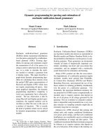
7.4.4 Experimental Results
In this section, early results (1986) in robust road recognition with multiple redun-
dant feature extraction in eight windows are shown. In these windows, displayed in
Figure 7.17, one microprocessor Intel 8086 each extracted several edge candidates
for the lane boundaries (see figure).
On the left-hand side of the lane, the
tar filling in the gaps between the
plates of concrete that form the road
surface, gave a crisp edge; however,
disturbances from cracks and dirt on
the road were encountered. On the
right-hand side, the road boundary
changed from elevated curbstones to
a flat transition on grass expanding
onto the road.
Features accepted for representing
the road boundary had to satisfy con-
tinuity conditions in curvature (head-
ing change over arc length) and
colinearity. Deviations from ex-
pected positions according to spatio-
temporal prediction also play a role:
Figure 7.17. Multiple oriented edge extrac-

tion in eight windows with first-generation,
real-time image processing system BVV2
[Mysliwetz 1990]
226 7 Beginnings of Spatiotemporal Road and Ego-state Recognition
Features with offsets larger than 3ı from the expected value, were discarded alto-
gether; the standard deviation ı is obtained from the error covariance matrix of the
estimation process. This conservative approach stabilizes interpretation; however,
one has to take caution that unexpected real changes can be handled. Especially in
the beginning of the estimation process, expectations can be quite uncertain or
even dead wrong, depending on the initially generated hypothesis. In these cases it
is good to have additional potential interpretations of the feature arrangement
available to start alternative hypotheses. At the time of the experiments described
here, just one hypothesis could be started at a time due to missing computing
power; today (four orders of magnitude in processing power per microprocessor
later!), several likely hypotheses can be started in parallel.
In the experiments performed on a campus road, the radius of curvature of about
140 m was soon recognized. This (low-speed) road was not designed as a clothoid;
the estimated C
1hm
parameter even changed sign (dotted curve in Figure 7.18a
around the 80 m mark). The heading angle of the vehicle relative to the road tan-
gent stayed below 1° (Figure 7.18b) and the maximum lateral offset y
V
was always
less than 25 cm (Figure 5.18c). The steering angle (Figure 5.18d) corresponds di-
rectly to road curvature with a bit of a lead due to the look-ahead range and feed-
forward control.
Figure 7.18. Test results in autonomous driving on unmarked campus–road: Transition
from straight to radius of curvature § 140 m. (a) Curvature parameters, (b) vehicle
heading relative to the road (<~ 0.9°), (c) lateral offset (< 25 cm), (d) steering angle

(time integral of control input). Speed was ~ 30 km/h.
0 20 40 Distance in meters 140
R = 140 m
0 20 40 Distance in meters 140
0 20 40 Distance in meters 140
0 20 40 Distance in meters 140
y
V
= 0.25 m
Ȝ = 2°
Ȝ = 0°
ȥ
V
= 1°
ȥ
V
= í1°
0
0
(a)
(b)
(c)
(d)
8 Initialization in Dynamic Scene Understanding
Two very different situations have to be distinguished for initialization in road
scenes: (1) The vehicle is being driven by a human operator when the visual per-
ception mode is switched on, and (2) the vehicle is at rest somewhere near the road
and has to find the road on its own. In the latter, much more difficult case, it has
sufficient time to apply more involved methods of static scene recognition. This
latter case will just be touched upon here; it is wide open for future developments.

It is claimed here that 3-D road recognition while driving along a road is easier
than with a static camera if some knowledge about the motion behavior of the ve-
hicle carrying the camera is given. In the present case, it is assumed that the
egovehicle is an ordinary car with front wheel steering, driving on ordinary roads.
Taking the known locomotion measured by odometer or speedometer into account,
integration of measurements over time from a single, passive, monocular, 2-D im-
aging sensor allows motion stereointerpretation in a straightforward and computa-
tionally very efficient way.
With orientation toward general road networks, the types of scenes investigated
are the human-built infrastructure “roads” which is standardized to some extent but
is otherwise quasi-natural with respect to environmental conditions such as lighting
including shadows, such as weather, and possible objects on the road; here, we
confine ourselves just to road recognition. The bootstrap problem discussed here is
the most difficult part and is far from being solved at present for the general case
(all possible lighting and weather conditions). At the very first start of the vision
process, alleviation for the task, of course, is the fact that during this self-
orientation phase no real-time control activity has to be done. Several approaches
may be tried in sequence; during development phases, there is an operator check-
ing the results of recognition trials independently. Solution times may lie in the
several-second range instead of tens of milliseconds.
8.1 Introduction to Visual Integration for Road Recognition
Some aspects of this topic have already been mentioned in previous chapters. Here,
the focus will be on the overall interpretation aspects of roads and how to get
started. For dynamic scene understanding based on edge and stripe features, the
spatial distribution of recognizable features has to be combined with translational
and rotational motion prediction and with the laws of central projection for map-
ping spatial features into the image plane. The recursive visual measurement proc-
ess fits the best possible parameters and spatial state time histories to the data
measured.
228 8 Initialization in Dynamic Scene Understanding

These estimates satisfy the motion model in the sense of least-squares errors
taking the specified (assumed) noise characteristics into account. Once started, di-
rect nonlinear, perspective inversion is bypassed by prediction-error feedback. To
get started, however, either an initial perspective inversion has to be done or an in-
tuitive jump to sufficiently good starting values has to be performed somehow,
from which the system will converge to a stable interpretation condition. On stan-
dard roads in normal driving situations, the latter procedure often works well.
For hypothesis generation, corresponding object databases containing both mo-
tion characteristics and all aspects geared to visual feature recognition are key ele-
ments of this approach. Tapping into these databases triggered by the set of fea-
tures actually measured is necessary for deriving sufficiently good initial values for
the state variables and other parameters involved to get started. This is the task of
hypothesis generation to be discussed here.
When applying these methods to complex scenes, simple rigid implementation
will not be sufficient. Some features may have become occluded by another object
moving into the space between the camera and the object observed. In these cases,
the interpretation process must come up with proper hypotheses and adjustments in
the control parameters for the interpretation system so that feature matching and in-
terpretation continues to correspond to the actual process happening in the scene
observed. In the case of occlusion by other objects/subjects, an information ex-
change with higher interpretation levels (for situation assessment) has to be organ-
ized over time (see Chapter 13).
The task of object recognition can be achieved neither fully bottom-up nor fully
top-down exclusively, in general, but requires joint efforts from both directions to
be efficient and reliable. In Section 5.5, some of the bottom-up aspects have al-
ready been touched upon. In this section, purely visual integration aspects will be
discussed, especially the richness in representation obtained by exploiting the first-
order derivative matrix of the connection between state variables in 3-D space and
features in the image (the Jacobian matrix; see Sections 2.1.2 and 2.4.2). This will
be done here for the example of recognizing roads with lanes. Since motion control

affects conditions for visual observation and is part of autonomous system design
in closed-loop form, the motion control inputs are assumed to be measured and
available to the interpretation system. All effects of active motion control on visual
appearance of the scene are predicted as expectations and taken into account before
data interpretation.
8.2 Road Recognition and Hypothesis Generation
The presence of objects has to be hypothesized from feature aggregations that may
have been collected in a systematic search covering extended regions of the image.
For roads, the coexistence of left- and right-hand side boundaries in a narrow range
of meaningful distances (say, 2 to 15 m, depending on the type of road) and with
low curvatures are the guidelines for a systematic search. From the known eleva-
tion of the camera above the ground, the angle of the (possibly curved) “pencil tip”
in the image representing the lane or road can be determined as a function of lane
8.2 Road Recognition and Hypothesis Generation 229
or road width. Initially, only internal hypotheses are formed by the specialist algo-
rithm for road recognition and are compared over a few interpretation cycles taking
the conventionally measured egomotion into account (distance traveled and steer-
ing angle achieved); the tracking mode is switched on, but results are published to
the rest of the system only after a somewhat stable interpretation has been found.
The degree of confidence in visual interpretation is also communicated to inform
the other perception and decision routines (agents).
8.2.1 Starting from Zero Curvature for Near Range
Figure 7.14 showed some results with a search region of six horizontal stripes. Re-
alistic lane widths are known to be in the range of 2 to 4.5 m. Note that in stripes 3
and 4, no edge features have been found due to broken lines as lane markings (in-
dicating that lane changes are allowed). To determine road direction nearby robus-
tly, approximations of tangents to the lane borderlines are derived from features in
well separated stripes (1, 2, and 5 here). The least-squares fit on each side (dashed
lines) yields the location of the vanishing point (designated P
i

here). If the camera
is looking in the direction of the longitudinal axis of the vehicle (ȥ
KV
= 0), the off-
set of P
i
from the vertical centerline in the image represents directly the scaled
heading angle of the vehicle (Figure 7.6). Similarly, if a horizonline is clearly visi-
ble, the offset of P
i
from the horizon is a measure of the pitch angle of the camera
ș
K
. Assuming that ș
K
is 0 (negligibly small), Equation 7.40 and its derivative with
respect to range L
i
can be written
2
( ) / ; / /  
B
i i zK i Bi i zK i
z L fkH L dz dL fkH L
.
(8.1)
Similarly, for zero curvature, the lateral image coordinate as a function of range
L
i
and its derivative become from Equation 7.37,

>
@
,
,
2
() ( /2 )/ ȥȥ;
/(/2)/.
 r   
   r 
lr
lr
Bi i y V i V VK
Bi i y V i
yL fk b yL
dy dL f k b y L
(8.2)
Dividing the derivative in Equation 8.2 by that in Equation 8.1 yields the ex-
pressions for the image of the straight left (+b) and right (íb) boundary lines;
/(/2)(/)/
/(/2)(/)/
  

;
.
B
lB V yz K
Br B V y z K
dy dz b y k k H
dy dz b y k k H
(8.3)

Both slopes in the image are constant and independent of the yaw angles ȥ (see
Figure 7.6). Since z is defined positive downward, the right-hand boundary–
coordinate increases with decreasing range as long as the vehicle offset is smaller
than half the lane width; at the vanishing point L
i
= , the vertical coordinate z
Bi
is
zero for ș
K
= 0. The vehicle is at the center of the lane when the left and right
boundary lines are mirror images relative to the vertical line through the vanishing
point.
Assuming constant road (lane) width on a planar surface and knowing the cam-
era elevation above the ground, perspective inversion for the ranges L
i
can be done
in a straightforward manner from Equation 8.1 (left);
/ 
izk
LfkHz
Bi
.
(8.4)
230 8 Initialization in Dynamic Scene Understanding
Equation 8.2 immediately yields the lumped yaw angle ȥ for L
i
ĺ  as
VVK
ȥ = ȥȥ ()/  f

B
iy
yL fk.
(8.5)
These linear approximations of road boundaries usually yield sufficiently accu-
rate values of the unknown state variables (y
V
and ȥ
V
) as well as the parameter lane
width b for starting the recursive estimation process; it can then be extended to fur-
ther distances by adding further search stripes at smaller values z
Bi
(higher up in the
image). The recursive estimation process by itself has a certain range of conver-
gence to the proper solution, so that a rough approximate initialization is sufficient,
mostly. The curvature parameters may all be set to zero initially for the recursive
estimation process when look-ahead distances are small. A numerical example will
be shown at the end of the next section.
8.2.2 Road Curvature from Look-ahead Regions Further Away
Depending on the type of road, the boundaries to be found may be smooth (e.g.,
lane markings) or jagged [e.g., grass on the shoulder (Figure 7.16) or dirt on the
roadside]. Since road size in the image decreases with range, various properly sized
edge masks (templates) are well suited for recognizing these different boundary
types reliably with the method CRONOS (see Section 5.2). Since in the near range
on roads, some a priori knowledge is given, usually, the feature extraction methods
can be parameterized reasonably well. When more distant regions are observed,
working with multiple scales and possibly orientations is recommended; a versatile
recognition system should have these at its disposal. Using different mask sizes
and/or sub–sampling of pixels as an inverse function of distance (row position in

the vertical direction of the image) may be a good compromise with respect to effi-
ciency if pixel noise is low. When applying direction-sensitive edge extractors like
UBM (see Section 5.3), starting from the second or third pyramid level at the bot-
tom of the image is advisable.
Once an edge element has been found, it is advisable for efficient search to con-
tinue along the same boundary in adjacent regions under colinearity assumptions;
this reduces search intervals for mask orientations and search lengths. Since lanes
and (two-lane) roads are between 2 and 7 m wide and do have parallel boundaries,
in general, this gestalt knowledge may be exploited to find the adjacent lane mark-
ing or road boundary in the image; mask parameters and search regions have to be
adjusted correspondingly, taking perspective mapping into account. Looking al-
most parallel to the road surface, the road is mapped into the image as a triangular
shape, whose tip may bend smoothly to the left (Figure 7.16) or right (Figure 7.17)
depending on its curvature.
As a first step, a straight road is interpreted into the image from the results of
edge finding in several stripes nearby, as discussed in the previous section; in Fig-
ure 7.14 the dashed lines with the intersection point P
i
result. From the average of
the first two pairs of lane markings, lane width and the center of the lane y
LC
are
determined. The line between this center point and P
i
(shown solid) is the reference
line for determining the curvature offset ǻy
c
at any point along the road. Further
lane markings are searched in stripes higher up in the image at increasingly further
distances. Since Equation 7.37 indicates that curvature can best be determined

8.2 Road Recognition and Hypothesis Generation 231
from look-ahead regions far away, this process is continued as long as lane mark-
ings are highly visible. During this process, search parameters may be adapted to
the results found in the previous stripe. Let us assume that this search is stopped at
the far look-ahead distance L
f
.
Now the center point of the lane at L
f
is determined from the two positions of
the lane markings y
Brf
and y
Blf
. The difference of these values yields the lane width
in the image b
Bf
at L
f
(Equation 7.38). The point where the centerline of this search
stripe hits the centerline of the virtual straight road is the reference for determining
the offset due to road curvature ǻy
c
(L
f
) (see distance marked in Figure 7.14). As-
suming that the contribution of C
1hm
is negligible against that of C
0hm

, from Equa-
tion 7.24, ǻy
c
(L
f
) = C
0hm
·L
f
2
/2. With Equation 7.37 and the effects of y
V
and ȥ
taken care of by the line of reference, the curvature parameter can be estimated
from
2
0hm
ǻǻ ()
Cf CBf f y f
yyLfkCL   2
as
2
0hm
2 ǻǻ2
Cf f CBf f y
CyLyLf   k .
(8.6)
On minor roads with good contrast in intensity (as in Figure 7.16), the center of
the road far away may be determined better by region-based methods like UBM.
8.2.3 Simple Numerical Example of Initialization

Since initialization in Figure 7.16 is much more involved due to hilly terrain and
varying road width, this will be discussed in later chapters. The relatively easy ini-
tialization procedure for a highway scene while driving is discussed with the help
of Figure 7.14. The following parameters are typical for the test vehicle VaMoRs
and one of its cameras around 1990: Focal length f § 8 mm; scaling factors for the
imaging sensor: k
z
§ 50 pixels/mm and k
y
§ 40 pixels/mm; elevation of camera
above the ground H
K
= 1.9 m. The origin of the y
B
, zB
B
B image coordinates is selected
here at the center of the image.
By averaging the results from stripes 1 and 2 for noise reduction, the lane width
measured in the image is obtained as 280 pixels; its center lies at y
LC
= í4 pixels
and z
LC
= 65 pixels (average of measured values). The vanishing point P
i
, found by
intersecting the two virtual boundary lines through the lane markings nearby and in
stripe 5 (for higher robustness), has the image coordinates y
BP

= 11 and z
BP
= í88
pixels. With Equation 8.5, this yields a yaw angle of ȥ§ 2° and with Equation 7.40
for L
f
ĺ, a pitch angle of ș
K
§í12°. The latter value specifies with Equation
7.40 that the optical axis (z
B
= 0) looks at a look-ahead range LB
oa
(distance to the
point mapped into the image center) of
/tanș 1.9/0.22 8.6 m
oa K K
LH
.
(8.7)
For the far look-ahead range L
f
at the measured vertical coordinate z
Bf
= í55
pixel, the same equation yields with F = z
Bf
/(f·k
z
) = í0.1375

(1 tan ș )( tanș ) 22.3 m
fK K K
LH F F  
.
(8.8)
With this distance now the curvature parameter can be determined from Equa-
tion 8.6. To do this, the center of the lane at distance L
f
has to be determined. From
232 8 Initialization in Dynamic Scene Understanding
the measured values y
Brf
= 80 and y
Blf
= 34 pixels the center of the lane is found at
y
BLCf
= 57 pixels; Equations 7.38 and 8.8 yield an estimated lane width of b
f
= 3.2
m. The intersection point at L
f
with the reference line for the center of the virtual
straight road is found at y
BISP
= 8 pixel. The difference ǻy
CBf
= y
BLCf
– y

BISP
= 49
pixels according to Equation 8.6, corresponds directly to the curvature parameter
C
0hm
yielding
1
0hm CBf f y
ǻ 2 ( ) 0.0137 mCy Lfk

 ,
(8.9)
or a radius of curvature of R § 73 m. The heading change of the road over the look-
ahead distance is ǻȤ(L
f
) § C
0hm
· L
f
= 17.5°. Approximating the cosine for an angle
of this magnitude by 1 yields an error of almost 5%. This indicates that to deter-
mine lane or road width at greater distances, the row direction is a poor approxima-
tion. Distances in the row direction are enlarged by a factor of ~ 1/cos [ǻȤ(L
f
)].
Since the results of (crude) perspective inversion are the starting point for recur-
sive estimation by prediction-error feedback, high precision is not important and
simplifications leading to errors in the few percent range are tolerable; this allows
rather simple equations and generous assumptions for inversion of perspective pro-
jection. Table 8.1 shows the collected results from such an initialization based on

Figure 7.14.
Table 8.1. Numerical values for initialization of the recursive estimation process derived
from Figure 7.14, respectively, assumed or actually measured
Name of variable Symbol (dimension) Numerical value Equation
Gaze angle in yaw ȥ (degrees) 2 8.5
Gaze angle in pitch ș (degrees) í12 7.40
Look-ahead range (max) L
f
(meter) 22.3 8.8
Lane width b (meter) 3.35 7.38
Lateral offset from lane center y
V
(meter) 0.17 7.39
Road curvature parameter C
0hm
(meter
í1
) 0.0137 § 1/ 73 8.9
Slip angle ȕ (degrees) unknown, set to 0
C
1hm
(meter
í2
) unknown, set to 0
C
1h
(meter
í2
) unknown, set to 0
Steering angle Ȝ actually measured

Vehicle speed V (m/s) actually measured
Figure 8.1 shows a demanding initialization process with the vehicle VaMoRs at
rest but in almost normal driving conditions on a campus road of UniBwM near
Munich without special lane markings
[Mysliwetz 1990]. On the right-hand side,
there are curbstones with several edge features, and the left lane limit is a very nar-
row, but very visible tar-filled gap between the plates of concrete forming the lane
surface. The shadow boundaries of the trees are much more pronounced in inten-
sity difference than the road boundary; however, the hypothesis that the shadow of
the tree is a lane can be discarded immediately because of the wrong dimensions in
lateral extent and the jumps in the heading direction.
Without the gestalt idea of a smoothly curved continuous road, mapped by per-
spective projection, recognition would have been impossible. Finding and checking
single lines, which have to be interpreted later on as lane or road boundaries in a
8.3 Selection of Tuning Parameters for Recursive Estimation 233
separate step, is much more difficult than introducing essential shape parameters of
the object lane or road from the beginning at the interpretation level for single edge
features.
Figure 8.1. Initialization of road recognition; example of a successful instantiation of a
road model with edge elements yielding smoothly curved or straight boundary lines and
regions in between with perturbed homogeneous intensity distributions. Small local de-
viations from average intensity are tolerated (dark or bright patches). The long white
lines in the right image represent the lane boundaries for the road model accepted as
valid.
For verification of the hypothesis “road,” a region-based intensity or texture
analysis in the hypothesized road area should be run. For humans, the evenly ar-
ranged objects (trees and bushes) along the road and knowledge about shadows
from a deep-standing sun may provide the best support for a road hypothesis. In
the long run, machine vision should be able to exploit this knowledge as well.
8.3 Selection of Tuning Parameters for Recursive

Estimation
Beside the initial values for the state variables and the parameters involved, the
values describing the statistical properties of the dynamic process observed and of
the measurement process installed for the purpose of this observation also have to
be initialized by some suitable starting values. The recursive estimation procedure
of the extended Kalman filter (EKF) relies on the first two moments of the stochas-
tic process assumed to be Gaussian for improving the estimated state after each
measurement input in an optimal way. Thus, both the initial values of the error co-
variance matrix P
0
and the entries in the covariance matrices Q for system pertur-
bations as well as R for measurement perturbations have to be specified. These data
describe the knowledge one has about uncertainties of the process of perception.
In Chapter 6, Section 6.4.4.1, it was shown in a simple scalar example that
choosing the relative magnitude of the elements of R and Q determines whether the
update for the best estimate can trust the actual state x and its development over
time (relatively small values for the variance ı
x
2
) more than the measurements y
234 8 Initialization in Dynamic Scene Understanding
(smaller values for the variance of the measurements ı
y
2
). Because of the complex-
ity of interdependence between all factors involved in somewhat more complex
systems, this so called “filter tuning” is considered more an art than a science. Vi-
sion from a moving platform in natural environments is very complex, and quite
some experience is needed to achieve good behavior under changing conditions.
8.3.1 Elements of the Measurement Covariance Matrix R

The steering angle Ȝ is the only conventionally measured variable beside image
evaluation; in the latter measurement process, lateral positions of inclined edges
are measured in image rows. All these measurements are considered unrelated so
that only the diagonal terms are nonzero. The measurement resolution of the digi-
tized steering angle for the test vehicle VaMoRs was 0.24° or 0.0042 rad. Choos-
ing about one-quarter of this value as standard deviation (ı
Ȝ
= 0.001 rad), or the
variance as ı
Ȝ
2
= 10
í
6
, showed good convergence properties in estimation.
Static edge extraction to subpixel accuracy in images with smooth edges has
standard deviations of considerably less than 1 pixel. However, when the vehicle
drives on slightly uneven ground, minor body motion in both pitch and roll occurs
around the static reference value. Due to active road following based on noisy data
in lateral offset and heading angle, the yaw angle also shows changes not modeled,
since loop closure has a total lumped delay time of several tenths of a second. To
allow a good balance between taking previous smoothed measurements into ac-
count and getting sufficiently good input on changing environmental conditions, an
average pixel variance of ı
yBi
2
= 5 pixel
2
in the relatively short look-ahead range of
up to about 25 m showed good results, corresponding to a standard deviation of

2.24 pixels. According to Table 7.1 (columns 2 and 3 for L § 20 m) and assuming
the slope of the boundaries in the image to be close to ±45° (tan § 1), this corre-
sponds to pitch fluctuations of about one-quarter of 1°; this seems quite reasonable.
It maybe surprising that body motion is considered measurement noise; how-
ever, there are good reasons for doing this. First, pitching motion has not been con-
sidered at all up to now and does not affect motion in lateral degrees of freedom; it
comes into play only through the optical measurement process. Second, even
though the optical signal path is not directly affected, the noise in the sensor pose
relative to the ground is what matters. But this motion is not purely noise, since ei-
gen-motion of the vehicle in pitch exists that shows typical oscillations with re-
spect to frequency and damping. This will be treated in Section 9.3.
8.3.2 Elements of the System State Covariance Matrix Q
Here again it is generally assumed that the state variations are uncoupled and thus
only the diagonal elements are nonzero. The values found to yield good results for
the van VaMoRs by iterative experimental filter tuning according to
[Maybeck 1979;
Mysliwetz 1990]
are (for the corresponding state vector see Equation 9.17)
8.3 Selection of Tuning Parameters for Recursive Estimation 235
7574
91110910
Diag(10,10,10,10,
10 ,10 ,10 ,10 ,10 ).
Q

  

(8.10)
These values have been determined for the favorable observation conditions of
cameras relatively high above the ground in a van (H

K
= 1.8 m). For the sedan
VaMP with H
K
= 1.3 m (see Table 7.1) but much smoother driving behavior, the
variance of the heading angle has been 2 to 3 · 10
í
6
(instead of 10
í
7
), while the
variance for the lateral offset y
V
was twice as high (~ 2·10
í
4
) in normal driving; it
went up by another factor of almost 2 during lane changes
[Behringer 1996]. Work-
ing with Q as a constant diagonal matrix with average values for the individual
variances usually suffices. One should always keep in mind that all these models
are approximations (more or less valid) and that the processes are certainly not per-
fectly Gaussian and decoupled. The essential fact is that convergence occurs to
reasonable values for the process to be controlled in common sense judgment of
practical engineering; whether this is optimal or not is secondary. If problems oc-
cur, it is necessary to go back and check the validity of all models involved.
8.3.3 Initial Values of the Error Covariance Matrix P
0
In contrast to the covariance matrices Q and R which represent long-term statistical

behavior of the processes involved, the initial error covariance matrix P
0
deter-
mines the transient behavior after starting recursion. The less certain the initially
guessed values for the state variables, the larger the corresponding entries on the
diagonal of P
0
should be. On the other hand, when relatively direct measurements
of some states are not available but reasonable initial values can be estimated by
engineering judgment, the corresponding entries in P
0
should be small (or even
zero) so that these components start being changed by the estimation process only
after a few iterations.
One practically proven set of initial values for road estimation with VaMoRs is
0
rel V 0hm 1hm 1h 0vm 1vm
P = Diag(0.1, 0, 0.1, 0.1, 0.1, 0, 0, 0.1, 0),
corresp. to y C C C C C .Ȝȕȥ
(8.11)
This means that the initial values estimated by the user (zeros) for the slip angle
ȕ and the C
1
parameters in all curvature terms are trusted more than those derived
from the first measurements. Within the first iterations all values will be affected
by the transition matrix A and the covariance matrices Q and R (according to the
basic relations given in Equations 6.12, 6.16, and 6.17 or the corresponding ex-
pressions in sequential filtering).
From Figure 7.9, it can be seen, that during the initial acceleration phase (chang-
ing V in upper graph) horizontal curvature estimation is rather poor; only after

about 1 km distance traveled are the horizontal curvature parameters estimated in a
reasonable range (R  1 km according to
[RAS-L-1 1984]). This is partly due to us-
ing only 2 windows on one side, relatively close together like shown in Figure 7.7.
The detailed analysis of this nonstationary estimation process is rather involved
and not discussed here. It is one example of the fact that clean academic conditions
are hardly found in steadily changing natural environments. However, the idealized
methods (properly handled) may, nonetheless, be sufficient for achieving useful re-
236 8 Initialization in Dynamic Scene Understanding
sults, partly thanks to steady feedback control in a closed-loop action-perception
cycle, which prohibits short-term divergence.
8.4 First Recursive Trials and Monitoring of Convergence
Depending on the quality of the initial hypothesis, short-term divergence may oc-
cur in complex scenes; once a somewhat stable interpretation has been achieved,
the process is likely to continue smoothly. In order not to disturb the rest of the
overall system, the perception process for a certain object class should look at the
convergence behavior internally before the new hypothesis is made public. For ex-
ample, in Figure 8.2, the long shadow
from a tree in winter may be inter-
preted as a road boundary in one hy-
pothesis.
Starting with the vehicle at rest and
assuming that the vehicle is oriented
approximately in the road direction
near the center of the lane, knowledge
about usual lane widths leads to the
hypothesis marked by white line seg-
ments. When nothing can be assumed
about the subject’s position, other road
hypotheses cannot be excluded com-

pletely, e.g., one road side following
the shadow of the tree in front of the
vehicle. The road then could be as well
on the left-hand as on the right-hand
side of the shadow from the tree; for
the resulting feature positions expected
from this hypothesis, new measurement tasks have to be ordered. Features found or
not found then have to be judged in conjunction with the hypothesis.
Figure 8.2. Ambiguous situation for gen-
erating a good road hypothesis without
additional measurement data and higher
level reasoning or other input
Starting initialization under these conditions while the vehicle is being driven by
a human, a few most likely hypotheses should be set up in parallel and started in-
ternally (without giving results to the rest of the system or to the operator). Assum-
ing that the human driver guides the vehicle correctly, the system can prune away
the road models not corresponding to the path driven by observing the convergence
process of the other (parallel) hypotheses; while driving, all features from station-
ary, vertically extended objects in the environment of the road will move in a pre-
dictable way corresponding to ego speed. Those hypothesized objects, having large
prediction errors, a high percentage of rejected features, or that show divergence,
will be eliminated. This can be considered as some kind of learning in the actual
situation.
In the long run, road recognition systems do not have to recognize just the road
surface, possibly with lanes, but a much larger diversity of objects forming the in-
frastructure of different types of roads. During the search for initial scene recogni-
8.4 First Recursive Trials and Monitoring of Convergence 237
tion, all objects of potential interest for vehicle guidance should be detected and
correctly perceived. In Section 8.5, the road elements to be initialized in more ad-
vanced vision systems will be discussed; here we look first at some steps for test-

ing hypotheses instantiated.
8.4.1 Jacobian Elements and Hypothesis Checking
The Jacobian matrix contains all essential first-order information, how feature po-
sitions in an image (or derived quantities thereof) depend on the states or parame-
ters of the object descriptions involved. Analyzing the magnitude of these entries
yields valuable information on the mapping and interpretation process, which may
be exploited to control and adapt the process of hypothesis improvement.
8.4.1.1 Task Adjustment and Feature Selection for Observability
The basic underlying equation links the m vector dy of measurements (and thus the
prediction errors) to the n vector of optimal increments for the state variables and
parameters dx to be iterated:
dy C dx
(8.13)
If one column (index c) of the C matrix is zero (or its entries are very small in
magnitude), this means that all measured features do not (or hardly) depend on the
variable corresponding to index c (see Figure 8.3); therefore one should not try to
determine an update for this component dx
c
from the actual measurements.
In the case shown, features 1, 3, 6, and m = 8 depend very little on state component
x
c
(fourth column) and the other ones not at all; if prediction error dy
3
is large, this is
m vector Column index c Best update
of prediction (m × n)
to be found
errors Jacobian matrix C for state components
1

th c1 th th
2
th th th
c3 th th
r1 th r3 th rn th
th th
c6 th
6
th
0|| >İ 0 |İ | İ || >İ 0
|| >İ 0 || >İ 00|| >İ
.000|İ | İ ||>İ 0
|İ | İ 0|İ | İ 00|İ | İ
|| >İ 0 || >İ 000
.
000|İ | İ 00
0||>İ 0
.
r
m
dy

dy

dy

dy
dy
d
§·

¨¸
¨¸
¨¸
d
¨¸
dd d
¨¸

¨¸
¨¸
d
¨¸
¨¸
¨¸
¨¸
©¹
1
2
th th cm th
.
.
000
|| >İ 0 || >İ |İ | İ 00
c
n
dx
dx
dx
dx

§·
¨¸
§
·
¨¸
¨
¸
¨¸
¨
¸
¨¸
¨
¸
¨¸

¨
¸
¨¸
¨
¸
¨¸
¨
¸
¨¸
¨
¸
¨¸
¨¸
©
¹

¨¸
¨¸
d
©¹
Figure 8.3. Example of a degenerate Jacobian matrix with respect to measurement
values y
r
, y
6
and state component x
c
(each of the absolute values of H
ri
and H
ci
is be-
low a specific threshold, see text; || means magnitude of the corresponding value)
238 8 Initialization in Dynamic Scene Understanding
reflected in changes of dx
c
and especially in the state component (c + 1), here 5, since
this influences y
3
by a larger factor. However, if prediction error dy
6
is large, the only
way of changing it within the feature set selected is by adjusting x
c
; since the partial
derivative J

is small, large changes in x
6c c
will achieve some effect in error reduction.
This often has detrimental effects on overall convergence. Very often, it is better to
look for other features with larger values of their Jacobian elements, at least in column
c, to substitute them for y
6
.
However, since we are dealing with dynamic systems for which dynamic links
between the state variables may be known (integral relationships and cross-feeds), the
system may be observable even though entire columns of C are zero. To check
observability of all n components of a dynamic system, a different test has to be
performed. For systems with single eigenvalues (the case of multiple eigenvalues is
more involved), observability according to Kalman may be checked by using the
matrix of right eigenvectors V (defined by A·V = V·ȁ, where ȁ is the diagonal matrix
of eigenvalues of the transition matrix A of the dynamic system). By performing the
linear similarity transformation
' 
x
Vx
(8.14)
the linearized measurement equation becomes
.
' ' with 'dy C V dx C dx C C V   
(8.15)
If all elements of a column in the C’ matrix are small or zero, this means that all
features positions measured do not depend on this characteristic combination of state
variables or parameters. Therefore, no meaningful innovation update can be done for
this component of the eigenmotions. Maybe, due to other conditions in the future,
some new features will occur which may allow also to have an innovation update for

this component.
The case of almost vanishing columns or rows of the matrix C is shown in Figure
8.3 for row indices r and 6 and for column index c. Here, the H
i,j
mean numerically
small values in magnitude compared to the noise level in the system. If all entries in a
matrix row are small or zero, this means that the position in the image of the
corresponding feature does not depend on any of the state variables or parameters of
the object represented by the C matrix, at least under the current conditions. Therefore,
the feature may be discarded altogether without affecting the update results. This
reduces the workload for the numerical computation and may help in stabilizing the
inversion process buried in the recursion algorithm. Due to noise, a prediction error is
likely to occur which will then be interpreted as a large change in the state vector
because of the smallness of the C elements; this will be avoided by removing this
measurement value altogether, if the row vector in C has only very small entries.
The judgment of smallness, of course, has to be made with reference to the
dimension of the corresponding state variable. An angle in radians determining a
feature position at the end of a long lever (say several meters) has to be weighted
correspondingly differently compared to another variable whose the dimension has
been chosen in centimeter (for whatsoever reason). So-called “balancing” by proper
weighting factors for each variable may bring the numerical values into the same
numerical range required for meaningful selection of thresholds for the H
jl
to be
considered effectively zero.
To obtain good results, the thresholds of the C element values should be chosen
generously. This is good advice if it can be expected that with time the aspect
8.4 First Recursive Trials and Monitoring of Convergence 239
conditions will become more favorable for determining the corresponding variable
and if the prediction model is already sufficiently good for handling the observation

task meanwhile. In summary, checking the conditioning of the Jacobian matrix and
adapting the observation process before things go wrong, is a better way to go than
waiting until interpretation has already gone wrong.
8.4.1.2 Feature Selection for Optimal Estimation Results
If computing power available is limited, however, and the number of features “s”
measurable is large, the question arises which features to choose for tracking to get
best state estimation results. Say, the processor capability allows m features to be ex-
tracted, with m < s. This problem has been addressed in
[Wuensche 1986, 1987]; the fol-
lowing is a condensed version of this solution. Since feature position does not depend
on the speed components of the state vector, this vector is reduced x
R
(all correspond-
ing expressions will be designated by the index R).
To have all state variables in the same numerical range (e.g., angles in radians
and distances in meters), they will be balanced by a properly chosen diagonal scal-
ing matrix S. The equation of the Gauss-Markov estimator for the properly scaled
reduced state vector (of dimension n
R
) is
11 1
ˆˆ
įį {( ) ( ) } ( ) ( *)
TTT
RNR R R R
x
Sx S CS R CS CS R yy
 
         
,

(8.16)
where C
R
is the Jacobian matrix, with the zero-columns for speed components re-
moved; R is the diagonal measurement covariance matrix, and S is the scaling ma-
trix for balancing the state variables. With the shorthand notation
1/2
NR
CRC

S 
(8.17)
,
T
Cthe performance index J = | C | is chosen with the recursive formulation
NN
||
T
ii
i
J
CC 
¦
,
(8.18)
where C
i
is a 2 × n
R
matrix from C

N
corresponding to feature i with two positional
components each in the image plane:
12
1
13212 14
23
||| | ||||.
T
T
AA
J
AAAAA AA
AA

 
(8.19)
A
1
is diagonal and A
4
is symmetrical. This expression may be evaluated with 16
multiplications, 2 divisions, and 9 (m í 1) + 7 additions. For initialization, a com-
plete search with (s over m) possible feature combinations is performed. Later on,
in the real-time phase, a suboptimal but efficient procedure is to find for each fea-
ture tracked another one out of those not tracked that gives the largest increase in J.
Since one cycle is lost by the replacement, which leads to an overall deterioration,
the better feature is accepted only if it yields a new performance measure sensibly
larger than the old one:
Į ,

new old
J
J!
(8.20)
.
with Į =1+İ
The best suited value of H is of course problem dependent. Figure 8.4 shows an
experimental result from a different application area: Satellite docking emulated
with an air-cushion vehicle in the laboratory. Three corner features of a known
polyhedral object being docked to are to be selected such that the performance in-
240 8 Initialization in Dynamic Scene Understanding
dex for recognizing the relative egostate is maximized. The maneuver consists of
an initial approach from the right-hand side relative to the plane containing the
docking device (first 40 seconds), an intermediate circumnavigation phase to the
left with view fixation by rotating around the vertical axis, and a final phase of
homing in till mechanical docking by a rod is achieved
[Wuensche 1986]. At point 2
(~ 57 s) a self-occlusion of the side to be docked to starts disappearing on the left-
hand side of the body, leading to small spacing between features in the image and
possibly to confusion; therefore, these features should no longer be tracked (lower
left corner starts being discarded). Only at point 4a are the outermost left features
well separable again. In region 5, the features on the right-hand side of the body
are very close to each other, leading again to poor measurement results (confusion
in feature correlation). The performance index improves considerably when at
around 100 s both upper outer corners of the body become very discernible.
Figure 8.4. Selection of optimal feature combinations of an autonomous air-cushion ve-
hicle with the sense of vision: Approach (first 40 seconds), circumnavigation of the
polyhedral object with view fixation, and homing in for docking (last 20 seconds)
[Wuensche 1986]
time in seconds

In road traffic, similar but – due to rounded corners and unknown dimensions of
cars – more complicated situations occur for changing the aspect conditions of an-
other vehicle. Of course, looking straight from behind, the length of the vehicle
body cannot be determined; looking straight from the side, body width is non-
observable. For aspect conditions in between, the size of the body diagonal can be
estimated rather well, while width and length separately are rather unstable due to
8.5 Road Elements To Be Initialized 241
poor visibility of features on the rounded edges and corners of the body inside the
outer contour
[Schmid 1995]. This means that both shape parameters to be estimated
and promising features for recognition and tracking have to be selected in depend-
ence on the aspect conditions.
8.4.2 Monitoring Residues
A very powerful tool for hypothesis checking in the 4-D approach consists of
watching and judging residues of predicted features. If no features corresponding
to predicted ones can be found, apparently the hypothesis is no good. Since it is
normal that a certain percentage of predicted features cannot be found, the number
of features tried should be two to three times the minimum number required for
complete state estimation. More features make the measurement and interpretation
process more robust, in general.
If the percentage of features not found (or found with too large prediction er-
rors) rises above a certain threshold value (e.g., 30%), the hypothesis should be ad-
justed or dropped. The big advantage of an early jump to an object hypothesis is
the fact that now there are many more features available for testing the correctness.
Early starts with several (the most likely) different hypotheses, usually, will lead to
earlier success in finding a fitting one than by trying to accumulate confidence
through elaborate feature combinations (danger of combinatorial explosion).
8.5 Road Elements To Be Initialized
In the long run, road recognition systems do not have to recognize just the road
surface, possibly with lanes, but a much larger diversity of objects forming the in-

frastructure of different types of roads (see Table 8.2 below).
Lane markings do not just define the lanes for driving. Information about ma-
neuvering allowed or forbidden is also given by the type of marking: Solid mark-
ings indicate that this line is not to be crossed by vehicles in normal situations; in
case of a failure, these lines may be crossed, e.g., for parking the vehicle on the
road shoulder. Dashed markings allow lane changes in both directions. A solid and
a dashed line beside each other indicate that crossing this marking is allowed only
from the dashed side while forbidden from the solid side. Two solid lines beside
each other should never be crossed. In some countries, these lines may be painted
in yellow color regularly while in others yellow colors are spared for construction
sites.
Within lanes, arrows may be painted on the surface indicating the allowed driv-
ing directions for vehicles in the lane
[Baghdassarian et al. 1994]. Other more com-
plex markings on roads can be found when the number of lanes changes, either
upward or downward; typical examples are exits or entries on high-speed roads or
turnoffs to the opposite direction of driving (left in right-hand traffic and vice
versa).
242 8 Initialization in Dynamic Scene Understanding
Vertical poles at regular spacing along the road (25 or 50 m), sometimes with
reflecting glass inserts, are supposed to mark the road when the surface is covered
with snow, dirt, or leaves in the fall. The reflecting glass may have different colors
(e.g., in Austria) or shapes (in Germany) to allow easier discrimination of left and
right road boundaries further away. Availability of this background knowledge in
vision systems makes road recognition easier.
Guide rails along the road also help affirming a road hypothesis. They have nice
features, usually, with elongated horizontal edges and homogeneous areas (bands
of similar color or texture) in between. Since they stand up about a half meter
above the road surface and at a certain distance to the side, they are separated from
the road surface by irregular texture from vegetation, usually. At sharper bends in

the road, especially at the end of a straight high-speed section, often red and white
arrow heads are painted onto their surface, signaling the driver to slow down.
When no guide rails are there, special signs at the usual location of guide rails with
arrows in the direction of the upcoming curve, or triangular traffic signs with bent
arrows in elevated positions usual for traffic signs may be found for alerting the
driver. Machine vision allows autonomous vehicles to take advantage of all this in-
formation, put up initially for the human driver, without additional cost.
Table 8.2. Objects of road infrastructure to be recognized on or in the vicinity of a road
Name of object
(class)
Location rela-
tive to road
Characteristic shape
(2-D, 3-D
Colors
Road markings On the surface Lines (0.1 to 0.5 m wide; solid,
dashed - single or in pairs, rec-
tangles, arrows
Chite, yellow
Vertical poles Beside road Round, triangular cylinders
(spacing every 25 or 50 m)
Black, white or-
ange
Traffic regula-
tion signs
Beside or
above
Round, triangular, square, rec-
tangular, octagonal
White, red and

black, blue
Arrows On guide
rails, posts
Solid arrows, diagonal and
cross-diagonal stripes
White and red,
black
Traffic lights Beside or
above
Round, rectangles
(with bars and arrows)
Red, yellow,
green
Signs for
navigation
Beside or
above
Large rectangular White, blue, green
Signs for city
limits
Beside Large rectangular (some
with black diagonal bar)
Yellow, black,
white
Signs for con-
struction sites
On, beside or
above
Round, triangular, rectangular
with diagonal stripes

Yellow, black, red
Guide rails Above and
beside road
Curved steel bands Metal, white and
red
Reflecting nails On surface Shallow rounded pyramid Yellow, red
Tar patches On surface Any Black
Turnoff lane At either side Widening lane with arrow White, yellow
Road fork Splitting road Y-shape Different shades
or textures
Traffic sign recognition has been studied for a long time by several groups, e.g.,
[Estable et al. 1994; Priese et al. 1995; Ritter 1997]. The special challenge is, on one
8.6 Exploiting the Idea of Gestalt 243
hand, separating these traffic signs from other postings, and on the other, recogniz-
ing the signs under partial occlusion (from branches in summer and snow in win-
ter). Recognition of traffic and navigational signs will not be followed here since it
can be decoupled from road recognition proper. What cannot be decoupled from
normal road recognition is detecting “reflecting nails” in the road surface and rec-
ognizing that certain patches in the road surface with different visual appearance
are nonetheless smooth surfaces, and it does no harm driving over them. Stereovi-
sion or other range sensing devices will have advantages in these cases.
On the contrary, driving on poorly kept roads requires recognizing potholes and
avoiding them. This is one of the most difficult tasks similar to driving cross-
country. On unmarked roads of low order with almost no restrictions on road cur-
vature and surface quality, visual road (track) recognition of autonomous vehicles
has barely been touched. Mastering this challenge will be required for serious mili-
tary and agricultural applications.
8.6 Exploiting the Idea of Gestalt
Studies of the nature of human perception support the conclusion that perception is
not just to reflect the world in a simple manner. Perceived size is not the same as

physical size, perceived brightness is not the same as physical intensity, perceived
velocity is not physical velocity, and so on for many other perceptual attributes.
Moreover, the perception of composite stimuli often elicits interpretations which
are not present when the components are perceived separately. Or in other words,
“The whole is different from the sum of its parts”. The gestalt laws deal with this
aspect in greater detail. Some remarks on history:
Ernst Mach (1838–1916) introduced the concepts of space forms and time
forms. We see a square as a square, whether it is large or small, red or blue, in out-
line or as textured region. This is space form. Likewise, we hear a melody as rec-
ognizable, even if we alter the key in such a way that none of the notes are the
same. Motion processes are recognized by just looking at dots on the joints of ar-
ticulated bodies, everything else being dark
[Johansson 1973].
Christian von Ehrenfels (1859–1932) is the actual originator of the term gestalt
as the gestalt psychologists were to use it. In 1890, he wrote a book On Gestalt
Qualities. One of his students was Max Wertheimer to whom Gestalt Psychology
is largely attributed.
Wolfgang Köhler (1887–1967) received his PhD in 1908 from the University of
Berlin. He then became an assistant at the Psychological Institute in Frankfurt,
where he met and worked with Max Wertheimer. In 1922, he became the chair and
director of the psychology lab at the University of Berlin, where he stayed until
1935. During that time, in 1929, he wrote Gestalt Psychology. The original obser-
vation was Wertheimer’s, when he noted that we perceive motion where there is
nothing more than a rapid sequence of individual sensory events. This is what he
saw in a toy stroboscope he bought by chance at a train station and what he saw in
his laboratory when he experimented with lights flashing in rapid succession (like
244 8 Initialization in Dynamic Scene Understanding
fancy neon signs in advertising that seem to move). The effect is called the phi
phenomenon, and it is actually the basic principle of motion pictures!
If we see what is not there, what is it that we are seeing? One could call it an il-

lusion, but it is not a hallucination. Wertheimer explained that we are seeing an ef-
fect of the whole event, not contained in the sum of the parts. We see a coursing
string of lights, even though only one light lights up at a time, because the whole
event contains relationships among the individual lights that we experience as well.
This is exploited in modern traffic at construction sites to vividly convey the (un-
expected) trajectory to be driven.
In addition, say the gestalt psychologists, we are built to experience the struc-
tured whole as well as the individual sensations. And not only do we have the abil-
ity to do so, we have a strong tendency to do so. We even add structure to events
which do not have gestalt structural qualities.
In perception, there are many organizing principles called gestalt laws. The
most general version is called the law of Praegnanz. It is supposed to suggest being
pregnant with meaning. This law says that we are innately driven to experience
things in as good a gestalt as possible. “Good” can mean many things here, such as
regular, orderly, simplicity, symmetry, and so on, which then refer to specific ge-
stalt laws.
For example, a set of dots outlining the shape of an object is likely to be per-
ceived as the object, not as a set of dots. We tend to complete the figure, make it
the way it ‘should’ be, and finish it in the context of the domain perceived. Typical
in road scenes is the recognition of triangular or circular traffic signs even though
parts of them are obscured by leaves from trees or by snow sticking to them.
Gestalt psychology made important contributions to the study of visual percep-
tion and problem solving. The approach of gestalt psychology has been extended to
research in areas such as thinking, memory, and the nature of aesthetics. The Ge-
stalt approach emphasizes that we perceive objects as well-organized patterns
rather than an aggregation of separate parts. According to this approach, when we
open our eyes, we do not see fractional particles in disorder. Instead, we notice lar-
ger areas with defined shapes and patterns. The "whole" that we see is something
that is more structured and cohesive than a group of separate particles. That is to
say, humans tend to make an early jump to object hypotheses when they see parts

fitting that hypothesis.
In visual perception, a simple notion would be that to perceive is only to mirror
the objects in the world such that the physical properties of these objects are re-
flected in the mind. But is this really the case? Do we “measure” the scene we
watch? The following examples show that perception is different from this simple
notion and that it is more constructive. The nature of perception fits more with the
notion to provide a useful description of objects in the outside world instead of be-
ing an accurate mirror image of the physical world. This description has to repre-
sent features that are relevant to our behavior.
The focal point of gestalt theory is the idea of "grouping", or how humans tend
to interpret a visual field or problem in a certain way. The main factors that deter-
mine grouping are
 proximity - how elements tend to be grouped together depending on their spatial
closeness;
8.6 Exploiting the Idea of Gestalt 245
 similarity - items that are similar in some way tend to be grouped together;
 closure - items are grouped together if they tend to complete a shape or pattern;
 simplicity - organization into figures according to symmetry, regularity, and
smoothness.
In psychology, these factors are called the laws of grouping in the context of
perception. Gestalt grouping laws do not seem to act independently. Instead, they
appear to influence each other, so that the final perception is a combination of the
entire gestalt grouping laws acting together. Gestalt theory applies to all aspects of
human learning, although it applies most directly to perception and problem-
solving.
8.6.1 The Extended Gestalt Idea for Dynamic Machine Vision
Not only is spatial appearance of importance but also temporal gestalt (patterns
over time, oscillations, optical flow): Objects are perceived within an environment
according to all of their elements taken together as a global construct. This gestalt
or “whole form” approach has tried to isolate principles of

perception: seemingly
innate mental laws that determine the way in which objects are perceived.
This capability of humans, in general, has been exploited in designing roads and
their infrastructure for humans steering vehicles.
Road curvature is recognized from smooth bending of the “pencil tip”, also over
time, as when a road appears in video sequences taken by a camera in a vehicle
guided along the road. The steering angle needed to stay at the center of the lane
(road) is directly proportional to curvature; steering rate is thus linked to speed
driven (see Equations 3.10/3.11). However, continuously seeing the road is not
necessary for perceiving a smoothly curved road. When snow covers both road and
shoulders and there is no vertical surface profile perpendicular to the road
(everything is entirely flat so that there are no surface cues for recognizing the
road), humans are, nonetheless, able to perceive a smoothly curved road from poles
regularly spaced along the side of the road. Introduced standards of spacing are 25
m (on state roads) or every 50 m (on freeways designed for higher speeds). While
driving continuously at constant speed, each pole generates a smoothly curved tra-
jectory in the image; the totality of impressions from all poles seen thus induces in
the human observer the percept of the smoothly curved road. Technical systems
can duplicate this capability by application of sampled data theory in connection
with a proper road model, which is standard state of the art.
Similarly, guide rails or trees along the road can serve the same purpose. Guide
rails usually are elevated above the ground (~ 0.5 m) and allow recognizing curve
initiation at long distances, especially when marked with arrowheads (usually
black or red and white); while driving in a curve, the arrowheads give a nice (opti-
cal) feature flow field which the unstructured continuous guide rail is not able to
provide.
In Gestalt psychology, the mechanism behind these types of percepts is labeled
Principle of Totality. This is to say that conscious experience must be considered
globally (by taking into account all the physical and mental aspects of the
246 8 Initialization in Dynamic Scene Understanding

perceiving individual simultaneously) because the nature of the mind demands that
each component be considered as part of a system of dynamic relationships in a
task context. This is sometimes called the Phenomenon; in experimental analysis,
in relation to the Totality Principle, any psychological research should take
phenomena as a starting point and not be solely focused on sensory qualities.
In terms of the 4-D approach to dynamic machine vision, this means that early
jumps to higher level hypotheses for perception may be enlightening, shedding
new light (richer empirical background knowledge) for solving the vision task
based on impoverished (by perspective mapping) image data.
8.6.1.1 Spatial Components: Shape Characteristics
The semantics of perception are components not directly derived from bottom-up
signal processing; they originate from internal top-down association of relational
structures with derived image structures. Most reliable structures are least varying
based on a wealth of experience. It is claimed that 3-D space in connection with
central projection has to offer many advantages over 2-D image space with respect
to least variations (idealized as “invariance”) in the real world. This is the reason
why in the 4-D approach all internal representations are done in 3-D space directly
(beside continuous temporal embedding to be discussed later). From a collection of
features in the image plane, an immediate jump is made to an object hypothesis in
3-D space for a physical object observed under certain spatial aspect conditions
with the imaging process governed by straight light ray propagation. This may in-
clude mirroring.
Note that in this approach, the (invariant) 3-D shape always has to be associated
with the actual aspect conditions to arrive at its visual appearance; because of the
inertia of objects, these objects tend to move smoothly. Knowing 3-D shape and
motion continuity eliminates so called catastrophic events when in 2-D projection
entire faces appear or disappear from frame to frame.
From the task context under scrutiny, usually, there follows a strong reduction
in meaningful hypotheses for objects under certain aspect conditions from a given
collection of features observed. In order not to be too abstract, the example of

scene interpretation in road traffic will be discussed. Even here, it makes a large
difference whether one looks at and talks about freeway traffic, cross-country traf-
fic or an urban scene with many different traffic participants likely to appear. As
usual in the interpretation of real world dynamic scenes, two different modes of
operation can be distinguished: (1) The initial orientation phase, where the system
has to recognize the situation it is in (discussed here) and (2) the continuous track-
ing and control phase, where the system can exploit knowledge on temporal proc-
esses for single objects to constrain the range of interpretations by prediction-error
feedback (4-D part proper to be discussed later).
Certain Gestalt laws have been formulated by psychologists since humans can-
not but perceive groups of features in a preferred way: The law of proximity states
that objects near each other tend to be seen as a unit. A useful example in road
marking is the following: Parallel, tightly spaced double lines, one solid and the
other broken, are a single perceptual unit indicating that crossing this line is al-
8.6 Exploiting the Idea of Gestalt 247
lowed only from the side of the broken line and not from the other. Two solid lines
mean that crossing is never allowed, not even in critical situations.
The law of closure says that, if something is missing in an otherwise complete
figure, we will tend to add it. A circle or a rectangle, for example, with small parts
of their edges missing, will still be seen as a circle or a rectangle, maybe described
by the words “drawn with interrupted lines”; if these lines are interrupted regularly,
a specification such as “dashed” or “dash-dotted” is immediately understood in a
conversation between individuals if they have the geometric concept of circle or
rectangle at their disposal. For the outer rec-
tangle in Figure 8.5, the gap at the lower left
corner will be “closed” (maybe with a foot-
note like “one corner open”.
The law of similarity says that we will
tend to group similar items together, to see
them as forming a gestalt, within a larger

form. An example in road traffic may be rec-
ognizing wheels and vehicle bodies. Recog-
nizing the separate subparts may be ambigu-
ous. When they are assembled in standard
form, tapping knowledge about form and
function can help finding the correct hypotheses more easily. An idealized example
is given in Figure 8.6. Covering up the rest of the figure except the upper left part
(a), the graph could be read as the digit zero or the letter ‘o’ written in a special
form for usage in posters. If the additional hint is given that the figure shows a 3-D
body, most of us (with a multitude of wheeled vehicles around in everyday life)
would tend to see an axially symmetrical ring (tube for a wheel?) under oblique
viewing conditions; whether it is seen from the left or from the right side cannot be
decided from the simple graphic display.
Figure 8.5. The law of closure in
Gestalt psychology for completing
basic shapes (under perturbations?)
(d)
(c)
(a)
(b)
(e)
Part (b) shows two such objects side by side; they are perceived as separate
units. Only when in part (c) a very simple box-like objects is added, covering most
Figure 8.6. Percepts in road traffic: (a) An elliptically shaped, ring-like figure (could be
an axially symmetrical tube for tires under an oblique angle, seen either from the left or
the right). (b) A pair of shapes like (a) (see text); (c) adding a simple vehicle body ob-
scuring most of the three wheels, the arrangement of (a) and (b) turns into the percept of
a wheeled vehicle clearly seen from the rear left side (or the front right side!). (d) and
(e), adding minor details to (a) resolves ambiguity by spatial interpretation: d) is a twin-
wheel seen from the rear left while (e) is viewed from the rear right. [There is more

background knowledge available affirming the interpretations in (c) to (e), see text.]
248 8 Initialization in Dynamic Scene Understanding
of the three objects arranged as in parts a) and b), the percept immediately is that of
a cart seen from above, the left and the rear. The visible parts of the formerly sepa-
rate three objects now fit the two hypotheses of a vehicle with four wheels, seen ei-
ther (1) from the rear left or (2) from the front right; one wheel is self-occluded. In
case (1) it is the front right wheel, while in case (2) it is the rear right one. There is
no doubt that the wheels are both seen from the same side; this is due to the inter-
pretation derived from the rectangular box. In parts d) and e) of the figure, the ob-
ject from (a) has been supplemented with a differently looking surface representing
the contact area of the wheel to the ground. From this additional cue it is apparent
that the “tires” in (d) are seen from the rear left, while the one in (e) is seen from
the rear right (or vice versa, depending on the direction of travelling that is needed
for disambiguation). The twin-tires in (d) immediately induce the percept of a truck
since cars do not have this arrangement of wheels, in general.
The object on the upper surface of the vehicle body is also hypothesized as a
wheel in the perception process because it fits reasonably to the other wheels (size
and appearance). If not mounted on an axle, the pose shown is the most stable one
for isolated wheels. As a spare part, it also fits the functional aspect of standard us-
age. Quite contrary, the ellipses seen on the rear (front) side of the vehicle will not
be perceived as a wheel by humans, normally; at best, it is painted there for what-
ever reason. Note that except size, color, and pose it is identical to the leftmost
wheel of the vehicle seen only partially (the contact area of the tire to the ground is
not shown in both cases); nonetheless, the human percept is unambiguous. It is this
rich background of knowledge on form and function of objects that allows intelli-
gent systems easy visual perception.
Next, there is the law of symmetry. We tend to perceive objects as symmetrical
in 3-D space even though they appear asymmetrical in perspective projection.
Other vehicles tend to be seen as symmetrical since we are biased by previous ex-
perience; only when seen straight from the back or the front are they close to sym-

metrical, usually. Traffic signs of any shape (rectangular, circular, and triangular)
are perceived as symmetrical under any aspect conditions; knowledge about per-
spective distortion forces us to infer the aspect
conditions from the distortions actually seen.
The law of good continuation states that objects
arranged in either a straight line or a smooth curve
tend to be seen as a unit. In Figure 8.7, we distin-
guish two lines, one from A to B and another from
C to D, even though this graphic could represent
another set of lines, one from A to D and the other
from C to B. Nevertheless, we are more likely to
identify line A to B, which has better continuation
than the line from A to D, which has an obvious
discontinuity in direction at the corner. If the con-
text in which this arrangement appeared would
have been objects with corners of similar appear-
ance, continuity over time could invoke the other
interpretation as more likely. Bias from context is
known to have considerable influence.
A
B
C
D
Figure 8.7. The law of good
continuation tends to favor
‘two lines crossing’ as per-
cept (A-B crossing C-D) and
not two corners touching
each other (AD touches BC)
or (AC touches BD)

8.6 Exploiting the Idea of Gestalt 249
The idea behind these examples, and much of the gestalt explanation of things,
is that the world of our experiencing is meaningfully organized, to one degree or
another; we receive a better payoff taking these (assumed) facts into account.
The gestalt effect refers to the form–forming capability of our senses,
particularly with respect to the visual recognition of figures and whole forms
instead of just a collection of simple lines and curves. Key properties of gestalt
systems are emergence, reification, multistability, and invariance.
Emergence: Some parts are seen only after the
whole has been hypothesized. Reification is the
constructive or generative aspect of perception, by
which the experienced percept contains more
explicit spatial information than the sensory
stimulus on which it is based. For instance, based on
the fact that straight lines can be fit between the
centers of three black circles, the human observer
will see a (“Kaniza”) triangle in Figure 8.8, although
no triangle has actually been drawn.
We have noticed our vehicle perception system in
a highway scene overlooking two vehicles driving
side by side in front at almost constant speed, but
claiming a vehicle (for several cycles) in the space
between the vehicles; only after several cycles has
this misinterpretation been resolved by the system
through newly hypothesized vehicles at the correct location without intervention of
an operator.
Figure 8.8. The percept of
a white triangle, based on
an obscuration hypothesis
for three separate dark cir-

cular disks in triangular ar-
rangement
Multi-stability (or
Multi-stable perception) is the tendency of ambiguous
perceptual experiences to pop back and forth unstably between two or more
alternative interpretations. This is seen for example in the well-known
Necker cube
shown in Figure 8.9. It is even claimed that one cannot suppress this alternation by
conscious attention
[Pöppel et al. 1991]; this
indicates that hypothesis generation is not fully
dependent on one’s will.
This phenomenon of multiple interpretations
may not only happen in pictorial (snapshot) image
interpretation as shown, but also in image se-
quences with moving light dots. As psychologists
have shown, individuals tend to interpret some of
these sequences differently, depending on the
context discussed previously or on the personal
background of experience. A difficult problem
arises in interpreting a snapshot from an action by
just one single frame; the actual pose may occur
in several different action patterns. It is again
likely to find the correct interpretation only by re-
ferring to the context which may be inferred from some other components of the
image or which has to be known from a different source; this problem is often en-
Figure 8.9. The Necker cube
(wire frame) showing two
stable 3-D interpretations: Ei-
ther from top right above or

from left below the cube.