Dynamic Vision for Perception and Control of Motion - Ernst D. Dickmanns Part 13 pdf

11.3 Detecting and Tracking Moving Obstacles on Roads 345
the general case. Therefore, it is always recommended to take into account the best
estimates for the road state and for the relative state of other vehicles.
The last three columns in Figure 11.6 will be of interest for the more advanced
vision systems of the future exploiting the full potential of the sense of vision with
high resolution when sufficient computing power will be available.
It is the big advantage of vision over radar and laser range finding that vision al-
lows recognizing the traffic situation with good resolution and up to greater ranges
if multifocal vision with active gaze control is used. This is not yet the general state
of the art since the data rates to be handled are rather high (many gigabytes/second)
and their interpretation requires sophisticated software.
In the case of expectation-based, multi focal, saccadic vision (EMS vision) it
has been demonstrated that from a functional point of view, visual perception as in
humans is possible; until the human performance level is achieved, however, quite
a bit of development has still to be done. We will come back to this point in the fi-
nal outlook.
Due to this situation, industry has decided to pick radar for obstacle detection in
systems already on the market for traffic applications; LRF has also been studied
intensively and is being prepared for market introduction in the near future. Radar-
based systems for driver assistance in cruise control have been available for a few
years by now. Complementing them by vision for road and lane recognition as well
as for reduction of false alarms has been investigated for about the same time.
These combined systems will not be looked at here; the basic goal of this section is
to develop and demonstrate the potential of vertebrate-type vision for use in the
long run. It exploits exactly the same features as human vision does, and should
thus be sufficient for safe driving. Multisensor adaptive cruise control will be dis-
cussed in Section 14.6.3.
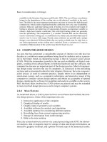
11.3.1 Feature Sets for Visual Vehicle Detection
Many different approaches have been tried for solving this problem since the late
1980s.
Regensburger (1993) presents a good survey on the task “visual obstacle

recognition in road traffic”. In
[Carlson, Eklundh 1990], an object detection method
using prediction and motion parallax is investigated. In
[Kuehnle 1991], the use of
symmetries of contours, gray levels and horizontal lines for obstacle detection and
tracking is discussed.
[Zielke et al. 1993] investigates a similar approach. Other ap-
proaches are the evaluation of optical flow fields
[Enkelmann 1990] and model-
based techniques like the one described below
[Koller et al. 1993]. Solder and
Graefe (1990)
find road vehicles by extracting the left, right and lower object
boundary using controlled correlation. An up-to-date survey on the topic may be
found in
[Masaki 1992++] or in the vision bibliography [ />Notes/bibliography/contents.html]. Some more recent papers are [Graefe, Efenberger
1996; Kalinke et al. 1998; Fleischer et al. 2002; Labayarde et al.2002; Broggi et al. 2004].
The main goal of the 4-D approach to dynamic machine vision from the begin-
ning has been to take advantage of the full spatiotemporal framework for internal
representation and to do as little reasoning as possible in the image plane and be-
tween frames. Instead, temporal continuity in physical space according to some
11 Perception of Obstacles and Vehicles
346
model for the motion of objects is being exploited in conjunction with spatial shape
rigidity in this “analysis-by-synthesis” approach.
Since high image evaluation rate had proven more beneficial in this approach
than using a wide variety of features, only edge features with adjacent average in-
tensity values in mask regions were used when computing power was very low
(see Section 5.2). With increasing computing power, homogeneously shaded blobs,
corner features, and in the long run, color and texture are being added. In any case,

perturbations both from the motion process and from measurements as well as
from data interpretation tend to change rapidly over time so that a single image in a
sequence should not be given too much weight; instead, filtering likely (maybe not
very precise) results at a high rate using motion models with low eigenfrequencies
has proven to be a good way to go. So, concentration on feature extraction was on
fast available ones with selection of those used guided by expectations and statisti-
cal data of the recursive estimation process running.
For this reason, image evaluation rates of less than about ten per second were
not considered acceptable from the beginning in the early 1980s; the number of
processors in the system and workload sharing had to be adjusted such that the
high evaluation rate was achievable. This was in sharp contrast to the approaches
to machine vision studied by most other groups around the globe at that time. Ac-
cumulated delay times could be handled by exploiting the spatiotemporal models
for compensation by prediction. These short cycle times, of course, left no great
choice of features to be used. On the contrary, even simple edge detection could
not be used all over the image but had to be concentrated (attention controlled!) in
those regions where objects of interest for the task at hand could be expected.
Once the road has been known from the specific perception loop for it, “obsta-
cles” could be only those objects in a certain volume above the road region, strictly
speaking only those within and somewhat to the side of the width of the wheel
tracks.
11.3.1.1 Edge Features and Adjacent Average Gray Values
Edge features are robust to changes in lighting conditions; maybe this is the reason
why their extraction is widespread in biological vision systems (striate cortex).
Edge features on their own have three parameters for specifying them completely:
position, orientation, and the value of the extreme intensity gradient. By associat-
ing the average intensity on one side of the edge as a fourth parameter with each
edge, average intensities on both sides are known since the gradient is the differ-
ence between both sides; this allows coarse area-based information to be included
in the feature.

Mori and Charkari (1993) have shown that the shadow underneath a vehicle is a
significant pattern for detecting vehicles; it usually is the darkest region in the en-
vironment. Combining this feature with knowledge of 3-D geometric models and
4-D dynamic scene understanding leads to a robust method for obstacle detection
and tracking.
[Thomanek et al. 1994; Thomanek 1996] developed the first vision sys-
tem capable of tracking a half dozen vehicles on highways in each hemisphere with
bifocal vision based on these facts in closed-loop autonomous driving. This ap-
proach will be taken as a starting point for discussing more modern approaches ex-
11.3 Detecting and Tracking Moving Obstacles on Roads 347
ploiting the increase in
computing power by at
least two orders of mag-
nitude (factor > 100)
since.
Figure 11.7 shows a
highway scene from a
wide-angle camera with
one car ahead in the sub-
ject’s lane. A search for
horizontal edge features
is performed in vertical
search stripes with
KRONOS masks of size
5 × 7 as indicated on the
right-hand side (see Sec-
tion 5.2). Due to missing computer performance in the early 1990s, the search
stripes did not cover the whole image below the horizon; evaluation cycle time was
80 ms (every second video field with the same index). Stripe width and spacing as
well as mask parameters had to be adjusted according to the detection range de-

sired. For improved resolution, there was a second camera with a telelens on the
gaze controlled platform (see Figure 1.3) with a viewing range about three times as
far (and a correspondingly narrower field of view) compared to the wide-angle
camera. This allowed using exactly the same feature extraction algorithms for ve-
hicles nearby and further away (see Figure 11.22 further below).
Find lower edge of a vehicle: About 30 search stripes of 100 pixels length have
been analyzed by shifting the correlation mask top-down to find close-to-horizontal
edge features at extreme correlation values. Potential candidates for the dark area
underneath the vehicle have to satisfy the criteria:
 The value of the mask response (correlation magnitude) at the edge has to be
above a threshold value (corr
min,uv
).
 The average gray value of the trailing mask region (upper part) has to be below
a threshold value (dark
min,uv
).
The first bullet requires a pronounced dark-to-bright transition, and the second one
eliminates areas that are too bright to stem from the shaded region underneath the
vehicle; adapting these threshold values to the situation actually given is the chal-
lenge for good performance. For tanker vehicles and low standing sun, the ap-
proach very likely does not work. In this case, the big volume above the wheels
may require area-based features for robust recognition (homogeneously shaded, for
example).
Generate horizontal contours: Edge elements satisfying certain gestalt conditions
are aggregated applying a known algorithm for chaining. The following steps are
performed, starting from the left window and ending with the right one:
1. For each edge element, search the nearest one in the neighboring stripe and store
the corresponding index if the distance to it is below a threshold value.
Search

direction
n
d
= 3
n
0
= 1
m
d
= 7
n
w
= 5
Mas
k
Figure 11.7. Detection of vehicle candidates by search of
horizontal edges in vertical search stripes below the hori-
on: Mask parameters selected such that several stripes
cover a small vehicle [Thomanek 1996]
z
11 Perception of Obstacles and Vehicles
348
2. Tag each edge element with the number count of previous corresponding ele-
ments (e.g., six, if the contour contains six edge elements up to this point).
Read starting point P
s
(y
s
, z
s

) and end point P
e
(y
e
, z
e
) of each extracted contour and
check the slope, whose magnitude |(z
e
– z
s
)/(y
e
– y
s
)| must be below a threshold for
being accepted (close to horizontal, see Figure 11.8).
If lines grow too long, they very likely stem from the shadow of a bridge or
from other buildings in the vicinity; they may be tracked as the hypothesis for a
new stationary object (shadow or discontinuity in surface appearance), but elimi-
nating them altogether will do no harm to tracking moving vehicles with speed al-
ready recognized. Within a few cycles, these elongated lines will have moved out
of the actual image. With knowledge of 3-D geometry (projection equations link
row number to range), the extracted contours are examined to see whether they al-
low association with
certain object classes:
Side constraints con-
cerning width must be
satisfied; likely height
is thereby hypothesized.

Contours starting
from inhomogeneous
areas inside the objects
(i.e., bumper bar or rear
window) are discarded;
they lie above the lower
shadow region (see Fig-
ure 11.9).
Determine lateral boundaries: Depending on the lateral position relative to the
lane driven in, the vertical object boundaries are extracted additionally. This is
done with an edge detector which exploits the fact that the difference in brightness
on the object and from the background is not constant and can even change sign; in
1. Chaining of
geometrically next
element
end
point
2. Numbering of edge
elements (each branch)
3. Elimination of shorter branch,
determine start and end point
start
point
Figure 11.8. Contour generation from edge elements observing gestalt ideas of nearness
and colinearity; below an upper limit for total contour length, only the longer one is kept
Figure 11.9. Extracted horizontal edge elements: The rec-
tangular group of features is an indication of a vehicle can-
didate; the lower elements (aggregated shadow region un-
der the car) allow estimation of the range to the vehicle
11.3 Detecting and Tracking Moving Obstacles on Roads 349

Figure 11.10, the wheels and fender
are darker than the light gray of the
road while the white body is brighter
than the road.
For this purpose, the gradient of
brightness is calculated at each posi-
tion in each image row, and its abso-
lute values are summed up over the
lines of interest. The calculated dis-
tribution of correlation values has
significantly large maxima at the ob-
ject boundaries (lower part of fig-
ure). The maxima of the accumu-
lated values yield the width of the
obstacle in the image; knowing
range and mapping parameters, ob-
stacle size in the real world is initial-
ized for recursive estimation and up-
dated until it is stable. With clearly
visible extremes as in the lower part
of Figure 11.10 the object width of
the real vehicle is fixed, and changes
in the image are from now on used
to support range estimation.
For vehicles driving in their own
lanes, the left and right object boundary must be present to accept the extracted
horizontal contour as representing an object. In neighboring lanes, it suffices to
find a vertical boundary on the side of the vehicle adjacent to their own lane to
prove the hypothesis of an object in connection with the lower contour. This means
that in the left lane, a vertical line to the right of the lower contour has to be found,

while in the right lane, one to the left has to be found for acceptance of the hy-
pothesis of a vehicle. This allows recognition of partially occluded objects, too.
The algorithm was able to detect and track up to five objects in parallel with four
INMOS Transputer® 222 (16 bit) for feature extraction and one T805 (32 bit) for
recursive estimation at a cycle time of 80 ms.
Figure 11.10. Determination of lateral
boundaries of a vehicle by accumulation of
correlation values at each position in each
single row of the lower part of the body with
a KRONOS-mask (n
w
= 1; n
d
= large). The
maxima of the accumulated values yield the
width of the obstacle in the image.
Histo-
gram
of
corre-
lation
max-
ima
from
single
rows
Pixel position
Applying these methods is a powerful tool for extracting vehicle boundaries in
monochrome images also for modern high-performance microprocessors. Adding
more features, however, can make the system more versatile with respect to type of

vehicle and more robust under strong perturbations in lighting conditions.
11.3.1.2 Homogeneous Intensity Blobs
Region-based methods, extracting homogeneously shaded or textured areas are of
importance especially for robust recognition of large vehicles. Color recognition
very much alleviates object separation in complex scenes with many objects of dif-
ferent colors. But just regions of homogeneous intensity shading alleviate object
separation considerably (especially in connection with other features).
11 Perception of Obstacles and Vehicles
350
In Figure 11.11 the homogeneously shaded areas of the road yield the back-
ground for detecting vehi-
cles with different inten-
sity blobs above a dark
region on the ground,
stemming from vehicle
shade underneath the
body. Though resolution
is poor (32 pixels per mel
and 128 per mask) and
some artifacts normal to
the search direction can
be seen, relatively good
hypotheses for objects are
derivable from this coarse
scale. Five vehicle candi-
dates can be recognized,
three of which are par-
tially occluded. The car
ahead in the same lane
and the bus in the right neighboring lane are clearly visible. The truck further

ahead in the subject’s lane can clearly be recognized by its dark upper body. For
the two cars in the left neighboring lane, resolution is too poor to recognize details;
however, from the shape of the road area, the presence of two cars can be hypothe-
sized. Low resolution allows higher evaluation frequency for limited computing
power.
Figure 11.11. Highway scene with many vehicles, ana-
lyzed with UBM method (see Section 5.3.2.4) in vertical
stripes with coarse resolution (22.42C) and aggregation
of homogeneous intensity blobs (see text).
Performing the search
on the coarse scale for
homogeneously shaded
regions in both vertical
and horizontal stripes
yields sharp edges in the
search direction; thus,
close to vertical blob
boundaries should be
taken from horizontal
search results while close
to horizontal boundaries
should be taken from ver-
tical search results.
Reconstructed image:
Coarse (4x4)
Fine
Coarse resolution
Figure 11.12. Highway scene similar to Figure 11.11
with more vehicles analyzed with UBM method in hori-
zontal stripes; the outer regions are treated with coarse

resolution (11.44R), while the central region (within the
white box) covering a larger look-ahead range above the
road, is analyzed on a fine scale (11.11R) (reconstructed
images, see text)
Figure 11.12 shows re-
sults from a row search
with different parameters
(11.44R) for another im-
age out of the same se-
quence (see bus in right
neighboring lane and the
11.3 Detecting and Tracking Moving Obstacles on Roads 351
dark truck in the subject’s lane). Here, however, the central part of the image, into
which objects further away on the road are mapped, is analyzed at fine resolution
giving full details (11.11R). This yields many more details and homogeneous in-
tensity blobs; the reconstructed image shown can hardly be distinguished from the
original image. A total of eight vehicle candidates can be recognized, six of which
are partially occluded. It can be easily understood from this image that large vehi-
cles like trucks and buses should be hypothesized from the presence of larger ho-
mogeneous areas well above an elevation of one wheel diameter from the ground.
For humans, it is immediately clear that in neighboring lanes, vehicles are recog-
nized by three wheels if no occlusion is present; the far outer front wheel will be
self-occluded by the vehicle body. All wheels will be only partially visible. This
fact has led to the development of parameterized wheel detectors based on features
defined by regional intensity elements
[Hofmann 2004].
Figure 11.13 shows the basic idea and the derivation of templates that can be
adapted to wheel diameter (including range) and aspect angle in pan (small tilt an-
gles are neglected because they enter with a cosine effect (§ 1)); since the car body
occludes a large part of the wheels, the lower part of the dark tire contrasting the

road to its sides is especially emphasized. For orthogonal and oblique views of the
near side of the vehicle, usually, the inner part of the wheel contrasts to the tire
around it; ellipticity is continuously adapted according to the best estimate for the
relative yaw (pan) angle.
Figure 11.13. Derivation of templates for wheel recognition from coarse shape repre-
sentations (octagon): (a) Basic geometric parameters: width, outer and inner visible ra-
dius of tire; (b) oblique view transforms circle into ellipses as a function of aspect angle;
(c) shape approximation for templates, radii, and aspect angle are parameters; (d) tem-
plate masks for typically visible parts of wheels [seen from left, right, § orthogonal, far
side (underneath body)]. Intelligently controlled 2-D search is done based on the exist-
ing hypothesis for a vehicle body (after [Hofmann 2004]).
The wheels on the near side appear in pairs, usually, separated by the axle dis-
tance in the longitudinal direction which lets the front wheel appear higher up in
the image due to camera elevation above the wheel axle. There is good default
knowledge available on the geometric parameters involved so that initialization
poses no challenge. Again, being overly accurate in a single image does not make
sense, since averaging over time will lead to a stable (maybe a little bit noisier) re-
11 Perception of Obstacles and Vehicles
352
sult with the noise doing no harm. To support estimation of the aspect conditions,
taking into account other characteristic subobjects like light groups in relation to
the license plate as regional features will help.
11.3.1.3 Corner Features
This class of features is especially helpful before a good interpretation of the scene
or an object has been achieved. If corner localization can be achieved precisely and
consistently from frame to frame, it allows determining feature flow in both image
dimensions and is thus optimally suited for tracking without image understanding.
However, the challenge is that checking consistency requires some kind of under-
standing of the feature arrangement. Recognition of complex motion patterns of ar-
ticulated bodies is very much alleviated using these features. For this reason, their

extraction has received quite a bit of attention in the literature (see Section 5.3.3).
Even special hardware has been developed for this purpose.
With the computing power nowadays available in general-purpose micro-
processors, corner detection can be afforded as a standard component in image
analysis. The unified blob-edge-corner method (UBM) treated in Section 5.3 first
separates candidate regions for corners in a very simple way from those for homo-
geneously shaded regions and edges. Only a very small percentage of usual road
images qualify as corner candidates depending on the planarity threshold specified
(see Figures 5.23 and 5.26); this allows efficient corner detection in real time to-
gether with blobs and edges. The combination then alleviates detection of joint fea-
ture flow and object candidates: Jointly moving blobs, edges, and corners in the
image plane are the best indicators of a moving object.
11.3.2 Hypothesis Generation and Initialization
The center of gravity of a jointly moving group of features tells us something about
the translational motion of the object normal to the optical axis; expanding or
shrinking similar feature distributions contains information on radial motion.
Changing relative positions of features other than expansion or shrinking carries
information on rotational motion of the object. The crucial point is the jump from
2-D feature distributions observed over a short amount of time to an object hy-
pothesis in 3-D space and time.
11.3.2.1 Influence of Domain and Actual Situation
If one had to start from scratch without any knowledge about the domain of the ac-
tual task, the problem would be hardly solvable. Even within a known domain (like
“road traffic”) the challenge is still large since there are so many types of roads,
lighting-, and weather conditions; the vehicle may be stationary or moving on a
smooth or on a rough surface.
It is assumed here that the human operator has checked the lighting and weather
conditions and has found them acceptable for autonomous perception and opera-
11.3 Detecting and Tracking Moving Obstacles on Roads 353
tion. When observation of other vehicles is started, it is also assumed that road rec-

ognition has been initiated successfully and is working properly; this provides the
system (via DOB, see Chapters 4 and 13) with the number and widths of lanes ac-
tually available. With GPS and digital maps onboard and working, the type of road
being driven is known: unidirectional or two-way traffic, motorway or general
cross-country/urban road.
The type of road determines the classes of obstacles that might be expected with
certain likelihood; the levels of likelihood may be taken into account in hypothesis
generation. Pedestrians are less likely on high-speed than on urban roads. Speed
actually being driven and traffic density also have an influence on this choice; for
example, in a traffic jam on a freeway with very low average speed, pedestrians are
more likely than in normal freeway traffic.
11.3.2.2 Three Components Required for Instantiation
In the 4-D approach, there are always three components necessary for starting per-
ception based on recursive estimation: (1) the generic object type (class and sub-
class with reasonable parameter settings), (2) the aspect conditions (initial values
for state components, and (3) the dynamic model as knowledge (or side constraint)
of evolution over time; for subjects, this includes knowledge of (stereotypical) mo-
tion capabilities and their temporal sequence. This latter component means an indi-
vidual capability for animation based on onsets of maneuvers visually observed;
this component will be needed mainly in tracking (see Section 11.3.3). However, a
passing car cutting into the vehicle’s lane immediately ahead will be perceived
much faster and more robustly if this motion behavior (normally not allowed) is
available also during the initialization phase, which takes about one half to one
second, usually.
Instantiation of a generic object (3-D shape): The first step always is to establish
good range estimation to the object. If stereovision or direct range measurements
are available, this information should be taken from these sources. For monocular
vision, this step is done with the row index z
Bu
of the lowest features that belong

most likely to the object. Then, the first part of the following procedure is, as it is
for static obstacles, to obtain initial values of range and bearing.
With range information and the known camera parameters, the object in the im-
age can be scaled for comparison with models in the knowledge base of 3-D ob-
jects. Homogeneously shaded regions with edges and corners moving in conjunc-
tion give an indication of the vehicle type. For example, in Figure 11.11, the car
upfront, the truck ahead of it (obscured in the lower part), and the bus upfront to
the right are easily classified correctly; the two cars in the lane to the left allow
only uncertain classification due to occlusion of large parts of them. Humans may
feel certain in classifying the car upfront left, since they interpret the intensity
blobs vertically located at the top and the center of the hypothesized car: The
somewhat brighter rectangle at the top may originate from the light of the sky re-
flected from the curved roof of the car. The bright rectangular patch between two
more quadratic ones a little bit darker halfway from the roof to the ground is inter-
preted as a license plate between light groups at each rear side of the car.
11 Perception of Obstacles and Vehicles
354
Figure 11.12 (taken a few frames apart from Figure 11.11) shows in the inner
high-resolution part that this interpretation is correct. It also can be seen by the
three bright blobs reasonably distributed over the rear surface that the car immedi-
ately ahead is now braking (in color vision, these blobs would be bright red). The
two cars in the neighboring lane beside the dark truck are also braking. (Note the
different locations and partial obscuration of the braking lights on the three cars
depending on make and traffic situation). Confining image interpretation for obsta-
cle detection to the region marked by the white rectangle (as done in the early
days) would make vehicle classification much more difficult. Therefore, both pe-
ripheral low-resolution and foveal high-resolution images in conjunction allow ef-
ficient and sufficiently precise image interpretation.
Aspect conditions: The vertical aspect angle is determined by the range and eleva-
tion of the camera in the subject vehicle above the ground. It will differ for cars,

vans, and trucks/buses. Therefore, only the aspect angle in yaw has to be derived
from image evaluation. In normal traffic situations with vehicles driving in the di-
rection of the lanes, lane recognition yields the essential input for initializing the
aspect angle in yaw.
On straight roads, lane width and range to the vehicle determine the yaw aspect
angle. It is large for vehicles nearby and decreases with distance. Therefore, in the
right neighboring lane, only the left-hand and the rear side can be seen; in the left
neighboring lane, it is the right-hand and rear side. Tires of vehicles on the left
have their dark contact area to the ground on the left side of the elliptically mapped
vertical wheel surface (and vice versa for the other side; see Figure 11.13d). As-
pects conditions and 3-D shape are closely linked together, of course, since both in
conjunction determine the feature distribution in the image after perspective pro-
jection, which is the only source available for dynamic scene understanding.
Dynamic model: The third essential component for starting recursive estimation is
the process model for motion which implements continuity conditions and knowl-
edge about the evolution of motion over time. This temporal component was the
one that allowed achieving superior performance in image sequence interpretation
and autonomous driving. As mentioned before, there are two big advantages in
temporal embedding:
1.
Known state variables in a motion process decouple future evolution from the
past (by definition); so there is no need to store previous images if all objects of
relevance are represented by an individual dynamic process model. Future evo-
lution depends only on (a) the actual state, (b) the control output applied, and (c)
on external perturbations. Items (b) and (c) principally are the unknowns while
best estimates for (a) are derived by visual observation exploiting a knowledge
base of vehicle classes (see Chapter 3).
2.
Disturbance statistics can be compiled for both process and measurement noise;
knowing these characteristics allows setting up a temporal filter process that

(under certain constraints) yields optimal estimates for open parameters and for
the state variables in the generic process model.
3. These components together are the means by which “the outside world is trans-
duced into an internal representation in the computer”. (The corresponding
question often asked in biological systems is, how does the world get into your
11.3 Detecting and Tracking Moving Obstacles on Roads 355
head?) Quite a bit of background knowledge has to be available for this purpose
in the computer process analyzing the data stream and recognizing “the world”;
features extracted from the image sequence activate the application of proper
parts of this knowledge. In this closed-loop process resulting in control output
for a real vehicle (carrying the sensors), feedback of prediction-errors shows the
validity of the models used and allows adaptation for improved performance.
The dynamic models used in the early days in [
Thomanek 1996] were the follow-
ing (separate, decoupled models for longitudinal and lateral translation, no rota-
tional dynamics):
Simplified longitudinal dynamics: The goal was to estimate the range and range
rate sufficiently well for automatic transition into and for convoy driving. Since the
control and perturbation inputs to the vehicle observed are unknown, a third-order
model with colored noise for acceleration as given in Equations 2.34 and 2.35 has
been chosen and proven to be sufficient [
Bar-Shalom, Fortmann 1988]. The noise
term n(t) is fed into a first-order system with time constant T
c
= 1/Į. The discrete
model then is (here ĭ = A)
k+1 k k k
2

[ /2, , 1].

T
k
xxDn
with D T T
)  

(11.10)
The discrete noise term n
k
is assumed to be a white, bias-free stochastic process
with normal distribution and expectation zero; its variance is
22
[] .
kq
En s
(11.11)
After [
Loffeld 1990] ı
q
should be chosen as the maximally expected acceleration
of the process observed.
Simplified lateral dynamics: Since the lateral positions of the vehicles observed
have only very minor effects on the subject’s control behavior, a standard second-
order dynamical model with the state variables, lateral position y
o
relative to the
subject’s (its own) lane center and lateral speed v
yo
are sufficient. The discrete
model then is

oo
v,k
yo yo
k+1 k
10
.
01 1
yy
T
n
vv
§· §·
§· §·

¨¸ ¨¸
¨¸ ¨¸
©¹ ©¹
©¹ ©¹
(11.12)
Again, the discrete noise term n
v,k
is assumed to be a white, bias-free stochastic
process with normal distribution, expectation equal to zero, and variance ı
qy
2
.
11.3.2.3 Initial State Variables for Starting Recursive Estimation
Figure 11.14 visualizes the transformation of the feature set marking the lower
bound of a potential vehicle into estimated positions for the vehicles in Cartesian
coordinates. In the left part of the figure, dark-to-bright edges of the dark area un-

derneath the vehicle in a top-down search are shown. For the near range, assuming
a flat surface is sufficient, usually. The tangents to the local lane markings are ex-
trapolated to a common vanishing point of the near range if the road is
curved.Since convergence behavior is good, usually, special care is not necessary
in the general case. From the right part of the figure, the bearing angles ȥ
i
to the
11 Perception of Obstacles and Vehicles
356
vehicle candidates can easily be determined. Initialization and feature selection for
tracking have to take the different aspect conditions in the three lanes into account.
Image
Spatial interpretation

3

2
The aspect graph in Figure 11.15 shows the distribution of characteristic fea-
tures as seen from the
rear left (vehicle in front in neighboring lane to the right).
The features detected, for which correspondence can be established most easily at
low computational cost, are the dark area underneath the vehicle and edge features
at the vehicle corners, front left and rear right (marked by bold letters in the fig-
ure). The configuration of rear groups of lights and license plate (dotted rectangle)
and the characteristic set of wheel parts are the features detectable and most easily
recognizable with additional area-based methods.
Figure 11.14. Transformation of image row, in which the lower edge of the dark
region underneath the vehicle appears, and of lateral position into Cartesian coordi-
nates, based on camera elevation above the ground assumed to be flat
Getting good estimates for the velocity components needed for each second-

order dynamic model is much harder. Again, trusting in good convergence behav-
ior leads to the easy solution, in which all velocity components are initialized with
zeros. Faster convergence may be achieved if an approximate estimation of the
Aspect hypothesis
instantiated:
Single vehicle
aspect graph:
straight
behind
Front left
front
right
SF
Veh
View from
rear left
left front
group of lights
left front
wheel
left rear group of lights
left rear
wheel
dark area under-
neath car, edges
right rear
wheel
right rear group
of lights
licence plate

elliptical
central blob
FL
SL
RL
SB
RR
straight from
front
edges
left front
edges rear right
dark tire below
body line
elliptical
central blob
group of blob features
SR
FR
dark tire below body
rear
right
Figure 11.15. Aspect conditions determine feature sets to be extracted for tracking. On
the same road in normal traffic, road curvature, distance, and the lane position relative to
the subject’s own lane are the most essential parameters; traffic moving in the same or in
the opposite direction exhibits rear/front parts of vehicles. On crossroads, views from the
side predominate. The situation shown is typical for passing a vehicle in right-hand traffic.
11.3 Detecting and Tracking Moving Obstacles on Roads 357
speed components can be achieved in the initial observation period of a few cycles;
this is especially true if the corresponding elements of measurement covariance are

set large and system covariance is set low (high confidence in the correctness of
the model).
11.3.2.4 Measurement Model and Jacobian Elements
There are two essentially independent motion processes in the models given: “Lon-
gitudinal” (x
o
, V
o
) and “lateral” states (y
o
, v
yo
) of the vehicle observed. Pitching mo-
tion of the vehicle has not yet been taken into account. However, if the sensors
(cameras) have no degree of freedom for counteracting vehicle motion in pitch,
this motion will affect visual measurement results appreciably (see Section 7.3.4).
Depending on acceleration and deceleration, pitch angles of several degrees (§ 0.05
mrad) are not uncommon; at 70 m distance, this value corresponds to a height
change in the real world of § 3.5 m for a point in the same row of the image.
Rough ground may easily introduce pitch vibrations with amplitudes around
0.25º (§ 0.005 mrad); at the same distance of 70 m, this corresponds to a 35 cm
height change or changes in look-ahead distances on flat ground in the range of 10
to 20 m (around 25 %). At shorter look-ahead distances, this sensitivity is much re-
duced; for example, at 20 m, the same vibration amplitude of 0.25° leads to look-
ahead changes of only about 1.3 m (6.5 %) for the test vehicle VaMP with camera
elevation H
K
= 1.3 m above the ground; larger elevations reduce this sensitivity.
Of course, this sensitivity enters range estimation directly according to Figure
11.14. A sensitivity analysis of Equation 7.19 (with distance ȡ instead of L

f
) shows
that range changes (ȡ/ș) as a function of pitch angle ș, and (ȡ/z
B
) as a function
of image row z
B
B
B go essentially with the square of the range:
(/ ) [/( )]
22
K
KzB
ǻ
ȡȡH ǻș + ȡ Hfk ǻz  .
(11.13)
This emphasizes analytically the numbers quoted above for the test vehicle
VaMP. Therefore, for large look-ahead ranges, one should not rely on average val-
ues for the pitch angle. If no gaze stabilization in pitch is available, it is recom-
mended to measure lane width at the position of the lower dark-to-bright feature
(Equation 11.2) and to evaluate an estimate for range assuming that lane width is
the same as determined nearby at distance L
n
and to compute the initial value x
o
us-
ing the pinhole camera model.
The measurement model for the width of the vehicle is given by Equation 11.3;
for each single vertical edge feature, the elements of the Jacobian matrix are
2

.
y
Bo o
y
ooo o
Bo o o
y
y
ooo o
fk
yy
fk
yyx x
yy y
fk f
xxx x

§·
w
w

¨¸
ww
©¹
§·
w
w
 
¨¸
ww

©¹
k
(11.14)
It can be seen that changes in lateral feature position in the image depend on
changes of state variables in the real world by
11 Perception of Obstacles and Vehicles
358
2
(/) /;
(/) /
Bo o o y o o
.
B
oo o yooo
yyǻyfkǻyx
yx
ǻ
xfkyǻxx
ww 
ww 
(11.15)
The second equation indicates that changes in range, 'x
o
, can be approximately
neglected for predicting lateral feature position since y
o
and 'x
o
<< x
o

, and range is
not updated from the prediction-error 'y
Bo
(no direct cross-coupling between lon-
gitudinal and lateral model necessary). However, since lateral position y
o
in the
first equation is updated by inverting the Jacobian element (y
Bo
/y
o
), small predic-
tion-errors 'y
Bo
in the feature position in the image will lead to large increments
'y
o
. Note that this sensitivity results from taking the camera coordinates only as
reference (x
o
). Determining y
oL
relative to the local road or lane has range x
o
cancel
out, and the lateral position of the vehicle in its lane can be estimated as much less
noise-corrupted.
11.3.2.5 Statistical Parameters for Recursive Estimation
The covariance matrices Q of the system models are required as knowledge about
the process observed to achieve good convergence in recursive estimation. The co-

variance matrix of the longitudinal model has been given as Equation 2.38. For the
lateral model, one similarly obtains
2
2
.
1
y qy
TT
Q ı
T
§·

¨¸
©¹
(11.16)
Optimal values for ı
q
2
have been determined in numerous tests with the real ve-
hicle in closed-loop performance driving autonomously. Stable driving with good
passenger comfort has been achieved for values ı
q
2
§ 0.1 (m/s
2
)
2
. A detailed dis-
cussion of this filter design may be found in
[Thomanek 1996].

The statistical parameters for image evaluation determine the measurement co-
variance matrix R. Errors in row and column evaluation are assumed to be uncorre-
lated. Since lateral speed is not measured directly but only reconstructed from the
model, the matrix R can be reduced to a scalar r with
22
r
r ı
(11.17)
as the variance of the feature extraction process. For the test vehicle VaMP with
transputers performing feature localization to full pixel resolution (no subpixel in-
terpolation) and with only 80 ms cycle time, best estimation results were achieved
with ı
r
2
= 2 pixel
2
[Thomanek 1996].
11.3.2.6 Falsification Strategies for Hypothesis Pruning
Computing power available in the early 1990s allowed putting up just one object
hypothesis for each set of features found as a candidate. The increase in computa-
tional resources by two to three orders of magnitude in the meantime (and even
more in the future) allows putting up several likely object hypotheses in parallel.
This reduces delay time until stable interpretation and a corresponding internal rep-
resentation has been achieved.
11.3 Detecting and Tracking Moving Obstacles on Roads 359
The early jump to full spatiotemporal object hypotheses in connection with
more detailed models for object classes has the advantage that it taps into the
knowledge bases with characteristic image features and motion models without
running the risk of combinatorial feature explosion as in a pure bottom-up ap-
proach putting much emphasis on generating “the most likely single hypothesis”.

Each hypothesis allows predicting new characteristic features which can then be
tested in the next image taking into account temporal changes already predictable.
Those hypotheses with a high rate and good quality of feature matches are pre-
ferred over the others, which will be deleted only after a few cycles. Of course, it is
possible that two (or even more) hypotheses continue to exist in parallel. Increas-
ingly more features considered in parallel will eventually allow a final decision;
otherwise, the object will be published in the DOB with certain parameters recog-
nized but others still open.
An example is a trailer observed from the rear driving at low speed; whether the
vehicle towing is a truck capable of driving at speeds up to say 80 km/h or an agri-
cultural tractor with a maximal speed of say 40 km/h cannot be decided until an
oblique view in a tighter curve or performing a lane change is possible; the length
of the total vehicle is also unknown. This information is essential for planning a
passing maneuver in the future. The oblique view uncovers a host of new features
which easily allow answering the open questions. Moving laterally in one’s own
lane is a maneuver often used for uncovering new features of vehicles ahead or for
discovering the reason for unexpectedly slow moving traffic.
Once the tracking process is running for an object instantiated, the bottom-up
detection process will rediscover its features independent of possible predictions.
Therefore, the main task is to establish correspondence between features predicted
and those newly extracted. A Mahalanobis distance with the matrix / for proper
weighting of the contribution of different features of a contour is one way to go.
Let the predicted contour of a vehicle be c*, the measured one c. Its position in
the image depends on (at least) three physical parameters: distance x, lateral posi-
tion y and vehicle width B. From the best estimates for these parameters, c* is
computed for the predicted states at the time of next measurement taking. The pre-
diction-errors c – c* are taken to evaluate the set of features of a contour minimiz-
ing the distance
1
(*) (*

T
dcc )
ȁ
cc

   .
(11.18)
From the features satisfying threshold values for (c – c*), those minimizing d
are selected as the corresponding ones. Proper entries for ȁ have to be found in a
heuristic manner by experiments.
It is the combination of robust simple feature extraction and high-level spatio-
temporal models with frequent bottom-up and top-down traversal of the representation
hierarchy that provides the basis for efficient dynamic vision. In this context, time and
motion in conjunction with knowledge about spatiotemporal processes constitute an
efficient hypothesis pruning device.
If both shape and motion state have to be determined simultaneously [
Schick 1992]
an interference problem may occur trading shape variations versus aspect conditions;
these problems have just been tackled and it is too early to make general statements on
favorable ways to proceed. But again, observing both spatial rigidity and (dynamic)
time constraints yields the best prospects for solving this difficult task efficiently.
11 Perception of Obstacles and Vehicles
360
11.3.2.7 Handling Occlusions
The most promising way to understand the actual traffic situation is to start with
road recognition nearby and track lane markings or road boundaries from near to
far. Since parts of these “objects” may be occluded by other vehicles or self-
occluded by curvatures of the road (both horizontally and vertically), obstacles and
geometric features on the side of the road have to be recognized in parallel for
proper understanding of “the scene”. The different types of occlusions require dif-

ferent procedures as proper behavior. A good general indicator for occlusion is
changing texture to one side of an edge and constant texture on the other side [
Gib-
son 1979
]; to detect this, high-resolution images are required, in general. This item
will be an important step for developing machine vision in the future with more
computing power available.
In curved and hilly terrain, driving safely until new viewing conditions allow
larger visual ranges is the only way to go. In flat terrain with horizontally curved
roads, there are situations where low vegetation obscures the direct view of the
road, but other vehicles can be recognized by their upper parts; their trajectory over
time marks the road. For example, if driving behind a slow vehicle, behind an on-
coming curve to the left, a vehicle in opposite traffic direction has been observed
over a straight stretch, and no indication of further vehicles is in sight, the vehicle
intending to pass should verify the empty oncoming lane at the corner and start
passing right away if the lane is free over a sufficiently long distance. (Note that
knowledge about one’s own acceleration capabilities as a function of speed and
visual perception capabilities for long ranges have to be available to decide this
maneuver.) In all cases of partial occlusion it is important to know characteristic
subparts and their relative arrangement to hypothesize the right object from the
limited feature set. Humans are very good in this respect, usually; the capability of
reliably recognizing a whole object from only parts of it visible is one important
ingredient of intelligence. Branches of trees or sticking snow partially occluding
traffic signs hardly hamper correct recognition of them. The presence of a car is
correctly assumed if only a small part of it and of one wheel are visible in the right
setting. Driving side by side in neighboring lanes, a proper continuous temporal
change of the gap between the front wheel (only partially visible) and fender of the
car passing will indicate an upcoming sideways motion of the car, probably need-
ing special attention for a while. Knowing the causal chain of events allows rea-
sonable predictions and may save time for proper reactions.

The capability of drawing the right conclusions from a limited set of informa-
tion visually accessible probably is one of the essential points separating good
drivers from normal or poor ones. This may be one of the areas in the long run
where really intelligent assistance systems for car driving will be beneficial for
overall traffic; early counteraction can prevent accidents and damage. (Our present
technical vision systems are far from the level of perception and understanding re-
quired for this purpose; in addition, difficult legal challenges have to be solved be-
fore application is feasible.)
11.3 Detecting and Tracking Moving Obstacles on Roads 361
11.3.3 Recursive Estimation of Open Parameters and Relative State
The basic method has been discussed in Chapter 6 and applied to road recognition
while driving in Chapters 7 to 10. In these applications, the scene observed was
static, but appeared to be dynamic due to relative egomotion, for which the state
has been estimated by prediction-error feedback. The new, additional challenge
here is to detect and track other objects moving to a large extent (but not com-
pletely) independent of egomotion of the vehicle carrying the cameras. For safe
driving in road traffic, at least half a dozen nearest vehicles in each hemisphere of
the environment have to be tracked, with visual range depending on the speed
driven. For each vehicle (or “subject”), a recursive estimation process has to be in-
stantiated for tracking. This means that about a dozen of these have to run in paral-
lel (level 2 of Figure 5.1).
Each of these recursive estimation processes requires the integration of visual
perception. The individual subtasks of feature extraction, feature selection, and
grouping as well as hypothesis generation have been discussed separately up to
here. The integration to spatiotemporal percepts has to be achieved in this step
now. In the 4-D approach, this is done in one demanding large step by directly
jumping to internal representations of 3-D objects moving in 3-D space over time.
Since these objects observed in traffic are themselves capable of perception and
motion control (and are thus “subjects” as introduced in Chapters 2 and 3), the
relevant parts of their internal decision processes leading to actual behavior also

have to be recognized. This
corresponds to an animation
process for several subjects in
parallel, based on observed
motion of their bodies. The
lower part of Figure 11.16
symbolizes the individual steps
for establishing a perceived
subject in the internal represen-
tation exploiting features and
feature flow over time (upper
part). The percept comes into
existence by fusing image data
measured with generic models
from object classes stored in a
background knowledge base;
using prediction-error feed-
back, this is a temporally ex-
tended process with adaptation
of open parameters and of state
variables in the generic models
describing the geometric rela-
tions in the scene.
Figure 11.16 Integration of visual perception for a
single object: In the upper part the coarsely
grained block diagram shows conventional feature
extraction, feature selection, and grouping as well
as hypothesis generation. The lower part imple-
ments the 4-D approach to dynamic vision, in
which background knowledge about 3-D shape

and motion is exploited for animating the spatio-
temporal scene observed in the interpretation
process.
‘Real world’
scene with
objects and
subjects
Feature selection
extraction grouping
Object hypothesis
generation (4-D):
shape, motion state
aspect conditions
4-D
models
instantiated:
objects &
subjects
Prediction
of motion
“Jacobian‘s”
perspective
mapping;
Predicted
2-D features
2-D features,
objects
tracked
Prediction error
feedback

cameras
Recognition of
perturbations
Parameter
adaptation
Toolbox
image feature
extractors
Generic object classes
Recursive estimation (4-D animation)
Initialization
Ideas of
‘Gestalt’
(methods)
11 Perception of Obstacles and Vehicles
362
11.3.3.1 Which Parameters/States Can Be Observed?
Visual information comes from a rather limited set of aspect conditions over a rela-
tively short period of time. Based on these poor conditions for recognition, either a
large knowledge base about the subject class has to be available or uncertainty
about the “object” perceived will be large. After hypothesizing an object/subject
under certain aspect conditions, the features available from image evaluation may
be complemented by additional features which should be visible if the hypothesis
holds. From all possible aspect conditions in road scenes, the dark area underneath
the vehicle and a left as well as a right vertical boundary on the lower part of the
body should always be visible; whether these vertical edges are detectable depends
on the image intensity difference between vehicle body and background. In gen-
eral, this contrast may be too small to be noticed at most over a limited amount of
time, due to changing background when the vehicle is moving. This is the reason
why these features (written bold in Figure 11.15) have been selected as a starting

point for object detection.
When another vehicle is seen from straight behind (SB), the vertical edges seen
are those from the left and right sides of the body; its length is not observable from
this aspect condition and is thus not allowed to be one of the parameters to be iter-
ated. When the vehicle is seen straight from the side (SR or SL), its width is unob-
servable but its length can be estimated (see Figure 11.6). Viewing the vehicle un-
der a sufficiently oblique angle, both length and width should be determinable;
however, the requirement is that the “inner” corner in the image of the vehicle is
very recognizable. This has not turned out to be the case frequently, and oscilla-
tions in the separately estimated values for length L and width B resulted
[Schmid
1995]
. Much more stable results have been achieved when the length of the diago-
nal (D = (L
2
+ B
2
)
1/2
) has been chosen as a parameter for these aspect conditions; if
B has been determined before from viewing conditions straight behind, the length
parameter can be separated assuming a rectangular shape and constant width. For
rounded car bodies, the real length will be a little longer than the result obtained
from the diagonal.
The yaw angle of a vehicle observed relative to the road is hard to determine
precisely. The best approach may be to detect the wheels and their individual dis-
tances to the lane marking; dividing the difference by the axle distance yields the
(tangent of the) yaw angle. Of the state variables, only the position components can
be determined directly from image evaluation; the speed components have to be
reconstructed from the underlying dynamic models.

It makes a difference in lateral state estimation whether the correct model with
Ackermann steering is used or whether independent second-order motion models
in both translational degrees of freedom and in yaw are implemented (independent
Newtonian motion components). In the latter case, the vehicle can drift sidewise
and rotate even when it is at rest in the longitudinal direction. With the Ackermann
model, these motion components are linked through the steering angle, which can
thus be reconstructed from temporal image sequences (see Section 14.6.1)
[Schick
1992]. If phases of standing still with perturbations on the vehicle body are encoun-
tered (as in stop-and-go traffic), the more specific Ackermann model is recom-
mended.
11.3 Detecting and Tracking Moving Obstacles on Roads 363
As mentioned before, motion of other vehicles can be described relative to the
subjet vehicle or relative to the local road. The latter formulation is less dependent
on perturbations of the vehicle body and thus is preferable.
11.3.3.2 Internal Representations
Each object hypothesis is numbered consecutively and stored with time of installa-
tion marking the observation period in local memory first for checking the stability
of the hypothesis; all parameters and valid state variables actually are stored in
specific slots. These are the same as available for publication to the system after
the hypothesis has become more stable within a few evaluation cycles; in addition,
information on the initial convergence/divergence process is stored such as: per-
centage of predicted features actually found, time history of convergence criteria
including variance, etc. When certain criteria are met, the hypothesis is published
to the overall system in the dynamic database (DDB, renamed later in dynamic ob-
ject database, DOB); all valid parameters and state variables are stored in specific
slots. Special state variables may be designated for entry into a ring buffer of size
n
RB
; this allows access to the n

RB
latest values of the variable for recognizing time
histories. The higher interpretation levels of advanced systems may be able to rec-
ognize the onset of maneuvers looking at the time history of characteristic vari-
ables.
Other subsystems can specify information on objects they want to receive at the
earliest date possible; these lists are formed by the DOB manager and sent to the
receiver cyclically. (To avoid time delays too large for stable reaction, some pre-
ferred clients receive the information wanted directly from the observation special-
ist in parallel.)
11.3.3.3 Controlling and Monitoring the Estimation Process
Each estimation process is monitored steadily through several goodness criteria.
The first is the count of predicted features for which no corresponding measured
feature could be established. Usually, obtaining a few times (factor of 2 to 4) the
amount of features minimally required for good observation is tried. If less than a
certain percentage (say, 70%) of these features has no corresponding feature meas-
ured, the measurement data are rejected altogether and estimation proceeds with
pure prediction according to the dynamic model. Confidence in the estimation re-
sults is decreased; Figure 11.17
shows a time history of the confi-
dence measure from
[Thomanek
1996]. After initialization, confi-
dence level V
E
is low for several
cycles until convergence data allow
lifting it to full confidence V
V
; if

not sufficiently many correspond-
ing features can be found, confi-
dence is decreased to level V
P
. If
this occurs in several consecutive
Figure 11.17. Time history of confidence
measure in object tracking: V
V
full confi-
dence, V
P
confidence from prediction only;
V
E
confidence for initialization.
Time
11 Perception of Obstacles and Vehicles
364
cycles, confidence is completely lost and goes to zero (termination of tracking).
Monitoring is done continuously for all tracking processes running. Figure
11.18 shows a schematic diagram implemented in the transputer system of the mid-
1990s. The vision system has two blocks: One for the front hemisphere with two
cameras using different focal lengths (lower left in figure with paths 1 and 2, the
latter not shown in detail) and one for the rear hemisphere (lower right, paths 3 and
4, only the latter is detailed). Objects are sorted and analyzed from near to far for
handling occlusions in a natural way. For each image stream, a local object ad-
ministration is in place. This is the unit communicating estimation results to the
rest of the system, especially to the global object administration process (center
top). Feature occlusion in the teleimage by objects tracked in the wide-angle im-

ages has to be resolved by this agent. It also has to check the consistency of the in-
dividual results; for example, very often the vehicle ahead in the subject’s lane is
the same in the tele- and the wide-angle image. In a more advanced system, this
fact should be detected automatically, and a single estimation process for this vehi-
cle should be fed with features from the two image streams; lacking time has not
allowed realizing this in the “Prometheus” project.
Figure 11.18. Structure and data flow of second-generation dynamic vision system for
ground vehicle perception realized with 14 transputers (see Figure 11.19) in test vehicles
VaMP and VITA_2 [Thomanek 1996]
1
2
3
4
Local
frame
storage
Local
frame
storage
Feature
extraction
Feature
extraction
Contour
generation
Contour
generation
tracking
front
tracking

rear
tracked
object
Correspondence
Monitor tracking
behavior and
data exchange
Hypothesis
generation
Prediction,
guidance of
feature ex-
traction,
verification
1 = teleimage front
2 = wide-angle front
3 = teleimage rear
4 = wide-angle rear
Newly
instantiated
object
Local
object
admini-
stration
(rear)
Object
tracked
Local
object

admini-
stration
(front)
Object
tracked
Background
data base
for generic
Object classes
Dynamic Object
data B
Global
object
admini-
stration
ase (DOB)
for single objects
actually tracked
Hypo-
thesis
gene-
ration
Video bus
11.3 Detecting and Tracking Moving Obstacles on Roads 365
All processes work with models from the background data base for generic ob-
ject classes (top left in Figure 11.18) and feed results into the DOB (top right).
This detailed visualization of the obstacle recognition subsystem has to be ab-
stracted on a higher level to show its embedding in the overall automatic visual
control system developed and demonstrated in the Prometheus-project; beside ob-
stacle recognition, other vision components for road recognition

[Behringer 1996],
for 3-D shape during motion
[Schick 1992], for moving humans [Kinzel 1995], and
for signal lights
[Tsinas 1997] were developed. This was the visual perception part
of the system that formed the base for the other components for viewing direction
control
[Schiehlen 1995], for situation assessment [Hock 1994], for behavior decision
[Maurer 2000], and for vehicle control [Brüdigam 1994].
Figure 11.19 shows the overall system, largely based on transputers, in coarse
resolution; this was the system architecture of the second-generation vision sys-
tems of UniBwM. Here, we just discuss the subsystem for visual perception with
the cameras shown in the upper left, and the road and obstacle perception system
shown in the lower right corners. The upper right part for system integra-
tion/locomotion control will be treated in Chapters 13 and 14.
Figure 11.19. Overall system architecture of second-generation vision system based
on transputers (about 60 in total) in VaMP: Road with lane markings and up to 12 ve-
hicles, 6 each in front and rear hemisphere, could be tracked at 12.5 Hz (80 ms cycle
time) with four cameras on two yaw platforms (top left). Blinking lights on vehicles
tracked could be detected with the subsystem in the lower left of the figure.
11.3.4 Experimental Results
From a system architecture point of view, the dynamic database (DDB) was intro-
duced as a flexible link and distributor allowing data input from many different de-
11 Perception of Obstacles and Vehicles
366
vices. These data were routed to all other subsystems; any type of processor or ex-
ternal computer could communicate with it.
Images used were 320 × 240 pixels from every fourth field (every second frame,
only odd or even fields); for intensity images coded with 1 byte/pixel, this yields a
video data input rate into the computer system of about 1MB/s for each video

stream. A total of 4 MB/s had to be handled on the two video buses for four cam-
eras shown in the bottom of the figure. The fields of view of these cameras looking
to the front and rear hemispheres can be seen for the front hemisphere in Figure
11.20; the ratio of focal lengths of the
cameras was about 3.2 which seemed
optimal for observing the first two rows
of vehicles in front. The system was de-
signed for perceiving the environment
in three neighboring lanes on high-
speed roads with unidirectional traffic.
A more detailed view of the vision
part of the system with the video busses
at the bottom, realized exclusively on
about four dozen transputers, can be
seen in Figure 11.21. In addition to the
intensity images, one color image
stream from one of the front cameras
could be sent via a separate third bus to
the unit for signal light analysis of the
vehicle directly ahead (lower left corner in Figure 11.19
[Tsinas 1997]).
wide angle
camera
dead zone
dead zone
Figure 11.20. Bifocal vision of test vehi-
cle VaMP for high-speed driving and
larger look-ahead ranges (see Figure 1.3
for a picture of the ‘vehicle eye’ with
two finger cameras on a single axis plat-

form for gaze control in yaw)
The arrangement of subsystems is slightly different in Figures 11.19 and 11.21.
The latter shows more organizational details of the distributed transputer system of
three different types (T2, T4, T8); the central role of the communication link (CL)
developed as a separate unit
[von Holt 1994] is emphasized here. Object detection
and tracking (ODT) has been realized with 14 transputers: Two T4 (VPU) for data
input from the two video buses, for data distribution into the four parallel paths
analyzing one image stream each and for graphic output of results as overlay in the
images (lower right); eight T2 (16-bit processors) performed edge feature extrac-
tion with the software package KRONOS written in the transputer programming
language “Occam” (see Section 5.2 and
[Thomanek, DDickmanns 1992]). Four T8
served as “object processors” (OP) on which recursive estimation for each object
tracked and the administrative functions for multiple objects were realized.
The data flow rate from ODT and RDT into the DDB compared to the video rate
is reduced by about two to three orders of magnitude (factor of ~ 300); in absolute
terms it is in the range 10 to 20 KB/s for ten vehicles tracked. With roughly 1 KB/s
data rate per vehicle tracked at 12.5 Hz, time histories of a few state variables can
easily be stored over tens of seconds for maneuver recognition at higher system
levels. (This function was not performed with the transputer system in the mid-
1990s.)
11.3 Detecting and Tracking Moving Obstacles on Roads 367
Figure 11.21. Realization of second-generation vision system with distributed tran-
sputers of various types: 16-bit processors (designated by squares) were used for fea-
ture extraction and communication; 32-bit processors (rectangles) were used for num-
ber crunching. Each transputer has four direct communication links for data exchange,
making it well suited for this type of distributed system.
Local object administration had to detect inconsistencies caused by two proc-
esses working on different images but tracking the same vehicle. It also had to

handle communication with other modules for exchanging relevant data. In addi-
tion, as long as a situation assessment module was not in operation on a higher
level, it determined the relevant object for “vehicle control” to react to.
11.3.4.1 Distance Keeping (Convoy Driving)
Figure 11.22 shows a situation with the test vehicle VaMP driving in the center
lane of a three-lane Autobahn; the vision system has recognized three vehicles in
each image (wide-angle at left, teleimage on the right). However, the vehicle in the
lane driven is the same in both images, while in the neighboring lanes, the vehicles
picked are different ones. Of course, in the general case, some vehicles in the
neighboring lanes may also be picked in both the wide angle and the teleimage;
these are the cases in which local supervision has to intervene and to direct the re-
cursive estimation loops properly. In the situation shown (left image), if the subject
vehicle passes the truck seen to the right nearby, but the black car in front remains
visible in the teleimage (say by a slight curve to the left), the case mentioned would
occur. The analysis process of the teleimage would have to be directed to track the
white truck (partially occluded here) in front of the black car; this car in turn would
have to be tracked in the wide-angle image.
11 Perception of Obstacles and Vehicles
368
Figure 11.22. Five objects tracked in front hemisphere; in the own lane only the vehi-
cle directly ahead can be seen (by both cameras). In neighboring lanes, the tele camera
sees the second vehicle in front.
It can be seen that the vehicles in front occlude a large part of the road bounda-
ries and of lane markings further away. It does not make sense that the road recog-
nition process tries to find relevant features in the image regions covered by other
vehicles; therefore, these regions are communicated from ODT to RDT and are ex-
cluded in RDT from feature search.
Range estimation by monocular vision has encountered quite a number of skep-
tical remarks from colleagues since direct range information is completely lost in
perspective mapping. However, humans with only one eye functional have no dif-

ficulty in driving a road vehicle correctly and safely.
To quantify precisely the accuracy achievable with monocular technical vision
after the 4-D approach, comparisons with results from laser range finders (LRF) in
real traffic have been performed. An operator pointing a single beam LRF steadily
onto a vehicle also tracked by the vision system was the simplest valid method for
obtaining relevant data.
Figure 11.23 shows a comparison between range estimation results with vision
(ODT as discussed above) and with a single-beam laser range finder pointed at the
object of relevance. It is seen that, except for a short period after the sign change of
relative speed (lower part), the agreement in range estimation is quite good (error
around 2% for ranges of 30 to 40 m). For ranges up to about 80 m, the error in-
creased to about 3%. The lower part in the figure shows that in the initial transient
phase, reconstruction (observation) of relative speed exhibits some large deviations
from reference values measured by a LRF. Speed from a LRF is a derived variable
also, but it is obtained at a higher rate and smoothed by filtering; it is certainly
more accurate than vision. The right subfigure for reconstructed relative speed
(range rate) shows strong deviations during the initial transient phase, starting with
the initial guess “0”, till about 2 seconds after hypothesis generation.
The heavy kinks at the beginning are due to changing feature correspondences
over time until estimation of vehicle width has stabilized. After the transients have
settled, visual estimation of relative speed is close to the LRF-based one. These re-
sults are certainly good enough for guiding vehicles only by machine vision; due to
increasing angles for decreasing range between features separated on the body sur-
face by a constant distance, accuracy of monocular vision becomes better when it
11.3 Detecting and Tracking Moving Obstacles on Roads 369
Figure 11.23. Comparison of results in range estimation between a single-beam, accu-
rately pointed laser range finder and dynamic monocular vision after the 4-D approach
in a real driving situation on a highway
is most needed (before a possible touch or crash). The results shown were achieved
in 1994 with the transputer system described.

Migration to new computer hardware: In 1995, replacing transputers within the
ODT block by PowerPC processors (Motorola 601) with more than ten times the
processing power per unit, evaluation frequency could be doubled (25 Hz) and the
number of processors needed was reduced by a factor of 6. With this system, the
long distance trip to the city of Odense, Denmark, mentioned in Section 9.4.2.5,
was performed in the same year.
Computing power per general-purpose microprocessor kept increasing at a fast
pace in these years. Since high-performance networks for fast data exchange be-
tween these processors also became available and the more powerful transputers
did not materialize, the third-generation vision system was started in 1997 on the
basis of “commercial-off-the-shelf “ (COTS) hardware, Intel Pentium®. One rack-
mounted PC system sufficed for doing the entire road recognition; a second was
used for bifocal obstacle recognition. Taking all pixels digitized in only odd or
even fields (25 Hz) allowed increasing the resolution to about 770 pixels per row
with 40 ms cycle time; vertical resolution was unchanged.
Object detection and tracking with COTS-PC systems: Figure 11.24 shows
tracking of two cars in a high-resolution image with edge extraction in intelligently
controlled search windows based on predictions from spatiotemporal models run-
ning at 40 ms cycle time (25 Hz).
The higher tracking frequency in connection with high image resolution allowed
robust tracking performance at moderate cost. For the same performance level, the
COTS system has been purchased for ~ 20% of the cost of a custom-designed sys-
tem used before.