Field and Service Robotics - Corke P. and Sukkarieh S.(Eds) Part 4 doc
Bạn đang xem bản rút gọn của tài liệu. Xem và tải ngay bản đầy đủ của tài liệu tại đây (3.99 MB, 40 trang )
The consistency model is described by an H
c
matrix equivalent to equation
4. This matrix is formed by iterating through each of the graph edges of the
mesh structure, where each edge yields one row of H
c
. For each edge, where
the edge is between nodes i and j :
H
c
row,i
= IH
c
row,j
= − I
(8)
The consistency model observation becomes an addition to Y , as in equation
5.
5.4 Two Dimensional Angular Profiles Demonstration
Figure 5 shows a demonstration of angular profiles from our flight vehicle and
ground vehicle. The patterned cylinder object was characterised according
to the metric area of the object as viewed from the (air or ground) borne
image sensor. This is a preliminary observable for demonstration of the esti-
mation structure. Figure 5(d) shows the separate contributions from the air
and ground vehicle, which are separate due simply to their differing angles
of elevation. The fusion of information from air and ground is simplified by
the use of angular profiles because they allow explicit differences in value at
viewing angles. Hence it is not required that features be absolutely identical
from air and ground. Figures 5(a) and 5(b) are shown at the same orienta-
tion. The peaks in profile information correspond to the groups of observation
points where multiple observations have been fused. Regions without observa-
tions take on an estimate obtained through the network of consistency models,
causing those regions to have non-zero information.
5.5 Information Theoretic Properties of Two Dimensional Angular
Profiles
One application of angular profiles is in causing information theoretic control
schemes [10] to explore multiple viewing angles of point features (in addi-
tion to spatial exploration over multiple features). This section describes the
properties of the determinants of the information matrices of angular profiles.
The entropic information i of an n -dimensional Gaussian variable with
Fisher information, Y and the mutual information I between two alternate
information matrices Y
a
and Y
b
are given by:
i =
1
2
log [(2πe)
n
| Y | ] I =
1
2
log
| Y
a
|
| Y
b
|
(9)
Angular profiles determinants have the followingproperties:
• After application of theconsistencymodel but before observations, | Y | =
0. Thismeans that Y retains the properties of anon-informativeprior
after application of the consistencymodel.
• Asingleobservation causes the determinant, | Y
b
| ,tobenon-zero.
Development of Angular Characterisation 113
114 P. Thompson and S. Sukkarieh
Easting MGA (m)
Northing MGA (m)
Cyclinder and View positions
6.1675 6.1676 6.1677 6.1678 6.1679
x 10
6
2.297
2.2975
2.298
2.2985
2.299
2.2995
2.3
2.3005
x 10
5
Cylinder
Ground Obs
Air Obs
(a)Cylinder Object location and air
and groundviewing positions
−1500−1000−500 0 500 1000 1500 2000
−1000
−500
0
500
1000
1500
2000
(b)Radius represents theprofile infor-
mation(inverse covariance). Theorien-
tation matches that of 5(a)
−4 −2 0 2
−2
−1
0
1
2
3
4
(c) Radius representsthe
profileestimate (Projected
area of theobject, m
2
)
-1
500
-1000
-500
0
500
1000
15
00
20
00
-5
00
0
500
1000
1500
-1000
-500
0
Air vehicle contributed
in
fo
rmatio
n
Ground vehicle contributed
information
(d) Radius representsthe profileinformation (in-
verse covariance). Informationpeakscorrespond to
air and ground observations
Fig. 5. Angular Profiles Demonstration
The mutualinformation properties of angular profiles are distinct from
those of three dimensional bearing onlypointlocalisation [10].Given asingle
observation,the next observationtomaximise information gain should be 180
degrees around theprofile. Asequence of adjacentobservations optimised for
information gain exploresall angles.
5.6 Other Applications and Extensions
Themethod of interpreting prediction modelsasdifferential observations used
here to develop atechnique for developing the consistencymodels forangu-
lar profiles can be applied to otherproblems in the estimation of spatially
distributed states. In particular,itcouldbeapplied to the estimation of the
trajectory of near-linearfeatures suchasfences, roads and rivers presented by
our fieldsite.
Interpreting prediction models as differential observations can also be ap-
plied to temporal estimation. It is a subject of future investigation to compare
this to other treatments of delayed and asequent data handling [11] and to
other smoothing formulations of estimation. [12]
Interpreting spatial consistency models and temporal prediction models as
differential observations (in space a time respectively) allows one to describe
consistency in space and time simultaneously. This provides a method for
simultaneously estimating spatially distributed random fields and providing
temporal smoothing (spatio-temporal estimation). This can be compared to
the spatial Kalman filtering described in [13] and [14].
It will be necessary to describe temporal process models for the angular
profiles, primarily to introduce uncertainty over time.
There are difficulties involved with handling observations of the angular
profile from uncertain angles. As described, the technique treats the angular
states as fixed on a set of angles around the object and so observations must
be subject to data association to choose the angle to update.
6 Conclusion and Future Work
In this paper we introduced our project and approach, described the vision
system and environment. We introduced a theory for the estimation of angular
profiles with demonstrations from simulation and field data.
In future developments we will be incorporating the image processing al-
gorithms and observation models necessary to observe angular profiles as de-
scribed here. We will be revising the decentralised data fusion system to allow
greater flexibility in the choice of states associated with each feature in order
to support the communication and fusion of angular profiles.
Feedback from the angular profile states and localisation states will need
to be used simultaneously for information theoretic decentralised control. As
discussed in section 5.5, an angular profile of a single feature has well behaved
properties in entropy and mutual information, causing decentralised control
algorithms to explore not only different positions in space but different an-
gles of view. However, implementing angular profiling alongside localisation
presents many challenges.
The technique of angular profiling is limited by the choice of the profiled
observable. For general vision based applications it may be preferable to fo-
cus on methods for estimating the three dimensional geometric structure and
colour or itensity of regions, rather than relying upon low dimensional remote
observables. However, the ability of angular profiles to provide an entropic
measure of angular information coverage is a relevant and beneficial feature.
Acknowledgments
This project is supported by the ARC Centre of Excellence programme, funded by
the Australian Research Council (ARC) and the New South Wales State Govern-
ment. This project is supported by BAE Systems, Bristol, UK.
Development of Angular Characterisation 115
116 P. Thompson and S. Sukkarieh
References
1. Salah Sukkarieh, Eric Nettleton, Jong-Hyuk Kim, Matthew Ridley, Ali Gokto-
gan, and Hugh Durrant-Whyte. The ANSER project: Data fusion across mul-
tiple uninhabited air vehicles. The International Journal of Robotics Research,
22(7-8):505–539, 2003.
2. Nadine Gobron, Bernard Pinty, Michel M Verstraete, Jean-Luc Widlowski, and
David J. Diner. Uniqueness of multiangular measurements. IEEE Transactions
on Geoscience and Remote Sensing , 40(7):1574 – 1592, 2002.
3. Eric Nettleton. Decentralised Architectures for Tracking and Navigation with
Multiple Flight Vehicles. PhD thesis, The University of Sydney, 2003.
4. Frank Dellaert, Steven M. Seitz, Charles E. Thorpe, and Sebastian Thrun. Struc-
ture from motion without correspondence. Proceedings of the IEEE Computer
Society Conference on Computer Vision and Pattern Recognition, 2:557 – 564,
2000.
5. D.T. Cole, S. Sukkarieh, A.H. Goktogan, H. Stone, and R. Hardwick-Jones. The
development of a real-time modular architecture for the control of uav teams.
In The 5th International Conference on Field and Service Robotics, July 2005.
6. Ed Waltz. Handbook of Multisensor Data Fusion. The Principles and Practice
of Image and Spatial Data Fusion. CRC Press, 2001.
7. Peter S. Maybeck. Stochastic models, estimation, and control, volume 1 of Math-
ematics in Science and Engineering. 1979.
8. Sebastian Thrun, Yufeng Liu, Daphne Koller, Andrew Y. Ng, Zoubin Ghahra-
mani, and Hugh Durrant-Whyte. Simultaneous localization and mapping with
sparse extended information filters. The International Journal of Robotics Re-
search, 23(7-8):693–716, 2004.
9. Pen-Olof Persson and Gilbert Strang. A simple mesh generator in matlab. SIAM
Review, 46(2):329 – 345, 2004.
10. Ben Grocholsky. Information-Theoretic Control of Multiple Sensor Platforms.
PhD thesis, Australian Centre for Field Robotics Department of Aerospace,
Mechatronic and Mechanical Engineering The University of Sydney, 2002.
11. Eric W. Nettleton and Hugh F. Durrant-Whyte. Delayed and asequent data in
decentralised sensing networks. Proceedings of SPIE - The International Society
for Optical Engineering, 4571:1 – 9, 2001. Decentralised sensing networks.
12. Robert F. Stengel. Optimal Control and Estimation. Dover, 1994.
13. K.V. Mardia, C. Goodall, E.J. Redfern, and F.J. Alonso. The kriged kalman
filter. Test (Trabajos de Estadstica) , 7(2):217–285, December 1998.
14. Noel Cressie and Christopher K. Wikle. Space time kalman filter. Encyclopedia
of Environmetrics, 2002.
Topological Global Localization for
Subterranean Voids
David Silver, Joseph Carsten, and Scott Thayer
Robotics Institute, Carnegie Mellon University, Pittsburgh, PA, USA
{ dsilver,jcarsten,sthayer} @ri.cmu.edu
Summary. The need for reliablemaps of subterranean spaces toohazardous for
humans to occupyhas motivated the developmentofrobotic mapping tools. For
suchsystemstobefully autonomous, they must be able to deal withall varietiesof
subterranean environments, including those containing loops. This paper presents an
approachfor an autonomous mobile robot to determine if the areacurrently being
exploredhas been previously visited. Combined with other techniques in topological
mapping, this approachwill allowfor the fully autonomous general exploration of
subterranean spaces. Data collected from aresearchcoal mine is used to experimen-
tally verify ourapproach.
1Introduction
In many parts of the world, abandonedmines present asignificant environ-
mental hazard. Toxic runoff, landslides,and subsidenceare just some of the
dangerspresentedbythesestructures.Inthe U.S. alone, there are tens of
thousands of abandoned mines [3] that threaten nearbysurfaceand subter-
ranean operations.The first steptowards combating this problemistoobtain
an accurate metric survey of the mine structure. Unfortunately,inmost cases
an accuratesurvey of the mine has either been lostornever existed.Taking
anew surveyofthe structure is oftenlimitedtoinspections via boreholes,
as abandoned mines are usually toodangerous for peopletoenter. Forthis
reason, robots have been proposed as amethod for mapping abandoned mines.
The Carnegie MellonSubterranean Roboticsgroup has undertakenthe
taskofdevelopingrobotic systems that can autonomously explore abandoned
mines or other hazardous subterraneanvoids. Theinitial effort led to the
developmentofasystem that canautonomously navigateand explore long
stretches of asingle mine portal [2]. More recentwork has focussed on ex-
panding mission profiles to include generalexplorationofmultipleintersect-
ing corridors.This led to asystemwhichcan detect and traverse multiple
corridors [13], but cannot determinewhen it has returned to apreviously
P. Corke and S. Sukkarieh (Eds.): Field and Service Robotics, STAR 25, pp. 117–128, 2006.
© Springer-Verlag Berlin Heidelberg 2006
118 D. Silver, J. Carsten, and S. Thayer
Fig. 1. Left: Groundhog, the currentrobotic platform of the mine mapping project.
Right:This map wasgeneratedfrom data acquired during experimentation and
utilizes offline globally consistent mapping techniques. It shows the highly cyclic
natureofroom-and-pillar mines.
visited corridor intersection from adifferentdirection. This constraintlimited
the environmentsexplored in [13]tothose whichdid not contain loops.
Thispaper presents amethod by which an autonomousmobile robot can
identify correspondences between intersections in subterranean environments,
allowing for autonomous loop closure and more general exploration. Our ap-
proachfor matching intersections is based on comparisons of both 2D and
3D range datalocal to eachintersection.The results of these comparisons
are then fedtoabinaryclassifier, whichproducesthe probabilityofamatch.
Such aclassifier can then be integrated into acompletesystemdesigned to
trackmultiple topological maphypotheses.
Theremainder of thispaper discusses therelevantdetails of our approach.
Section 2provides background into subterraneantopological exploration. Sec-
tion 3describesour technique, with experimental results presented in Section
4. We concludewithadiscussion and directions for future work.
2Subterranean TopologicalExploration
2.1Robotic Platform
Ourcurrentmine mapping platform is Groundhog (Figure 1), a700 kg
custom-builtATV-typerobot that is physicallytailoredfor operation in the
harsh conditions of abandoned mines. Groundhog’sprimary sensing consists
of 2SICK LMS-200 laserrange findersmountedinfrontand back. Eachhas
a180
◦
field of view,and is mounted on atilt mechanism with a60
◦
range.
Tilting each laser allows forthe acquisition of 3D range data. Groundhog
has been used extensively in both testand abandoned mine environments,
accruing hundreds of hours of mine navigation, including 8successful portal
entry experiments in the abandonedMathiesmine outside of Pittsburgh, PA.
Offline techniques have been used to generate globallyconsistent, large-scale
maps based on log datafrom these experiments. Forathoroughoverview of
the Groundhog system,see [2].
Topological Global Localization for Subterranean Voids 119
2.2 Topological Representations
Topological representations coincide nicely with the inherent structure of
room-and-pillar mines, which consist almost exclusively of narrow corridors
and corridor intersections (see Figure 1). A topological map is a graph repre-
sentation of an environment. The nodes of the graph correspond to distinct lo-
cations in the environment, and the edges correspond to direct paths between
two such locations. For mines, nodes and edges correspond to intersections
and corridors, respectively. This approach was used in [10] to allow a robot to
traverse known mine environments. Topological maps have also proven useful
in robotic exploration tasks of unknown environments [9]. Unexplored edges
in a topological map correspond to unexplored regions of the environment,
thus providing a mechanism for determining which region of the environment
to explore next.
The key components of a system designed for autonomous topological
exploration are:
• A method for traversing an edge in the environment until a node is reached.
• A method for detecting a node and its associated edges in the environment.
• A method for determining whether the currently sensed node has been
visited before, and if so which previously visited node it corresponds to
(this is the problem our current work strives to solve).
• A representation of the topological map and its associated uncertainty.
The first two components have been previously developed and tested in sub-
terranean environments, as described in the following sections.
2.3 Edge Traversal
Edge traversal is the first necessary component for autonomous topological
exploration. While traversing a single corridor, Groundhog utilizes the Sense-
Plan-Act (SPA) framework. While stationary, Groundhog tilts one of its lasers
to accumulate 3D range data from the space in front of it. This 3D point
cloud is used to generate a 2.5D cost map. Next, a goal pose is chosen that
will further Groundhog’s progress down the corridor (or turn it into a new
corridor). A path is planned to the goal pose by feeding the cost map into
a nonholonomic motion planner described in [13]. The planned path is then
traversed by Groundhog, and the whole process repeated. For a more detailed
description, see [2, 13].
2.4 Node Detection
A method for node detection is also critical to topological exploration.
Groundhog detects intersections in its environment by searching for nodes
of the generalized Voronoi diagram (GVD) [6]. Edges of the GVD represent
sets of points equidistant from 2 objects. Nodes of the GVD represent points
Fig. 2. Thedata collectedateachnode. Left: Groundhog approaching an inter-
section. Center: the 2D range data collected, as well as the detected node location
and radius. Right: the 3D range data collected.
equidistantfrom 3objects. Whiletraversing an edge,potential GVD nodes
are detectedusingaprocedure described in [15]. Each potential node is then
trackeduntil Groundhogdrives throughthe intersection to whichthe node
corresponds.The purposeofthis extra traverse is to obtain a2Dmap of the
environmentaround the node with afull 360
◦
coverage, as opposedtothe 180
◦
field of view of Groundhog’s lasers. Suchcoverageisachieved by combining
multiple laser scansfrom differentvantage points. This 360
◦
coverageisnec-
essary to determinewhetherthe intersectionjust traversedisworthexploring;
if the end of acorridor is already withinsensor range from the intersection
itself, it maynot be worth further exploration.This procedure alsoeliminates
largeconcavities that can appear as intersections whenfirst detected. After
anodehas been detected and verified,a3Dscan of theintersection is taken,
and Groundhogcontinues its exploration. The Voronoiradius (equidistance
value between thenodeand the objects that formed it), 2D map, and 3D scan
(Figure 2) are all storedfor later use.
2.5 Framework for Topological Uncertainty
Forsuccessful topological exploration, arobot must be abletodetermine if a
given node has been previouslyvisited. This determination canbemadebased
purely on the localtopology [7],orbycombining topological information with
rangedata or dataonnearbyfeatures. The techniques described in this paper
followthe latterapproach.
Regardless of the specifics of the node matchingapproach, its output will
be uncertain. There maybemultipleprevious nodes whichmatchthe current
node closely enough to be considered apossiblematch, and thefact that the
node maynever have been previously visited adds additionaluncertainty.A
framework is necessary for dealing with this uncertainty until the ambiguity
can be removed. Awidely adopted approach is to maintain multiple hypothe-
sesastothe correcttopology of theenvironment [8, 11,16]. The robot can
then either takeactions designed to explicityremove the ambiguity, or main-
tainmultiple hypotheses until the natural explorationbehavior of therobot
120 D. Silver, J. Carsten, and S. Thayer
Topological Global Localization for Subterranean Voids 121
produces enough additional information. In either case, the correct framework
can add additional robustness on top of the chosen node matching scheme.
3Subterranean Node Matching
We approachnodematching as atopological global localization problem.
When arobot arrives at anode N
i
alongedge E
i
,itcan localizeitself to
adiscrete subset of all possible states in theworld(the set of states located
at anode, oriented alonganedge). If the robot canproperly match N
i
and
E
i
to apreviously visited N
j
and E
j
,then it will have relocalized itself. If the
robot canproperly determine that N
i
has not been visited before,itwill still
have localized itself to the correct state, albeit astate thathas not previously
been visited.
To determine whether the current node N
i
matches aprevious node N
j
,
we use ahybrid approach based on both localtopology and range data(Figure
3). Local topological dataisrarely descriptive enoughtodetermine explicitly
whether twonodes match. However, it requiresessentially no preprocessing:
it is computationally inexpensivetodetermine whether N
i
and N
j
are of the
same degree. Forthis reason, localtopological dataisused to pare down the
number of prospective matches.
Forsimilarreasons, 2D as well as 3D range data is used. While 2D range
data is usually not descriptiveenoughtomakeanexplicit determination, it
is much cheaper to process than thefull 3D pointcloud,and can further pare
down the number of prospective matches. 2D datahas anotheradvantageun-
der our current setup: as described in Section 2.4,2Dinformation is collected
afull 360
◦
around theintersection. The additionalcoverage offered by 2D
dataoften provesquite useful in determining final matches.
Acommon approachfor determining whether arobot is revisiting alo-
cation is to explicitly search for featuresinthe local environment, and try
to matchthesefeatures to those that have been previously detected.How-
ever, subterranean spaces provide aunique challenge for featureextraction.
While suchspaces are oftenfeature rich,itishard to characterize thefeatures
exhibited. Featurescan very greatly in both type and scale, and so amore
robustapproach is needed. Forthis reason, our approachcompares nodes in a
manner which does not require explicit extraction of predetermined features.
3.1Comparison of Topological Properties
The first step of our node matching schemeistouse thetopological properties
of thedetected node N
i
to eliminate as many nonmatching nodes N
j
as possi-
ble. These topological properties are thedegree of the node and its associated
Voronoiradius. Another property we explored wasthe relativeorientations
of the edgesassociated withthe node. Previous work [12]has shown these
relative orientations to be quite susceptible to noise. This lackofrobustness
CompareNodes(N
i
,N
j
) :
if N
i
. degree = N
j
. degree then return 0
d ← N
i
. degree
if | N
i
. vRadius − N
j
. vRadius | >T
d
r
then return 0
P
2
← PositionOffsetBetweenNodes(N
i
,N
j
)
R
2
← MinimumErrorRotation(N
i
,N
j
,P
2
)
( MSE
2 D
,P
2
,R
2
) ← TrICP2D(N
i
. 2 D, N
j
. 2 D, P
2
,R
2
)
if MSE
2 D
>T
d
e
then return 0
( MSE
3 D
,P
3
,R
3
) ← TrICP3D(N
i
. 3 D, N
j
. 3 D, P
2
,R
2
)
E ← FormErrorVector(N
i
,N
j
,P
3
,R
3
)
return LogisiticRegression(E, d )
Fig. 3. Pseudocode for our node matching procedure
was also observed in our own experiments, and therefore this property was
not used. Instead, if N
j
has a different degree than N
i
, or the difference in
observed radii is more than a threshold T
r
, N
j
is eliminated as a candidate
match. T
r
is set relatively high, so as to ensure that no correct matches are
ever thrown out, while eliminating as many incorrect matches as possible in
a computationally inexpensive manner.
3.2 2D Map Matching
The next phase of node matching is to compare each node’s 2D local map.
Before the 2D maps can be compared, they must be properly aligned. Align-
ment of 2D point sets can be achieved using the Iterative Closest Point (ICP)
algorithm [4]. ICP assumes that each point in the data set corresponds to the
closest point in the model set. These correspondences are used to compute the
transformation between the two sets that minimizes the Mean Squared Error
(MSE). The correspondences are then recomputed, and the process iterates
until convergence.
Due to the manner in which our 2D maps are constructed, the assumption
that every point in the data set has a corresponding point in the model set is
often violated to a degree that degrades performance. Therefore, the Trimmed
Iterative Closest Point algorithm (TrICP) [5] is used instead. The key differ-
ence between ICP and TrICP is that TrICP assumes that only a proportion
ξ of the points in the data set correspond to points in the model set. At each
iteration, only ξK of the K points in the data set are used. The ξK points
used are those with the smallest squared distance to their corresponding point
in the model set. When unknown beforehand, ξ can be automatically set by
minimizing the function
ψ ( ξ ) = MSE ( ξ ) ξ
− (1+λ )
(1)
122 D. Silver, J. Carsten, and S. Thayer
Topological Global Localization for Subterranean Voids 123
where MSE ( ξ ) is the MSE of the ξK points with the smallest squared distance
to their corresponding point in the model set. The parameter λ balances the
tradeoff between using more points and increasing MSE. In [5], λ = 2.
Both ICP and TrICP require a fairly accurate initial alignment in order to
converge correctly. By framing node matching as a global localization prob-
lem, it is assumed that there does not exist a good long term estimate of
metric position. In practice, this is usually the case, as Groundhog’s online
position estimation is not stable over long distances (accurate metric maps
are produced offline). Since Groundhog’s perceived metric position can not be
used for an initial alignment, the locations of the nodes themselves are used.
Since each node is embedded into the environment, if the two local maps are
really of the same intersection, then the location of the Voronoi node in each
map corresponds to the same point in space, represented in different coor-
dinate frames. Setting the origin of each local map to be the corresponding
Voronoi point thus produces an initial alignment in position. However, the
orientation of each map relative to the node is still unknown. To fix the orien-
tation, TrICP is run 8 times, with the initial orientation of one map relative
to the other equally spaced at 45
◦
intervals. TrICP is able to overcome such
large errors in initial orientation because the error in initial position is small.
The final alignment that results in the smallest MSE is selected as the correct
2D alignment (Figure 4(a)).
The MSE of the final alignment (after recomputing ξ ) is compared against
a threshold T
e
. Just as with T
r
, T
e
is set to eliminate as many false matches
as possible, while not eliminating any correct matches.
3.3 3D Map Matching
The last phase of node matching uses the 3D range data gathered after each
node is detected. As with the 2D data, the 3D data must first be properly
aligned. The 3D alignment is also achieved using TrICP. The initial 3D align-
ment used for TrICP is based on the final 2D alignment. Using the 2D align-
ment between the candidate nodes, and the known position of each node
relative to the origin of the 3D scan, an initial 3D alignment is computed that
is fairly accurate in x, y and yaw. Just as running TrICP with only an initial x
and y allows the 2D alignment to converge to the correct orientation, running
TrICP with an initial x, y and yaw allows the 3D alignment to converge to
the correct z , roll, and pitch (Figure 4(b)).
In this phase, TrICP is run with one modification. Normally, ξ is computed
according to (1) once during the first iteration. Thus, ξ depends heavily on
the initial alignment. Since the initial alignment could have significant error
in 3 of the 6 degrees of freedom, ξ must be occasionally recomputed. For this
purpose, an additional loop is added around TrICP. After TrICP successfully
converges, ξ is recomputed based on the final alignment. The final alignment
is then fed back into TrICP as the new initial alignment. This process repeats
until the value of ξ converges.
(a)2Dalignment: Eachmap is centered around its Voronoi node,and then one
map is rotatedrelativetothe othertofind the minimumMSE alignment.
(b) 3D alignment: the 2D alignmentisused as theinitial 3D alignment ( left).
The ξN
d
closest points ( center)are then used to findthe final alignment
( right).
Fig. 4. 2D and 3D alignmentofrange data at an intersection
After each 3D alignmentiscomplete, an error vector E = { e
1
, , e
n
} is
producedfor eachprospective match N
i
↔ N
j
.The errorvector consists
of both 2D and3Derror measures.The 2D metrics are useddespite the
availability of 3D metrics, duetothe 360
◦
coverageof2Ddata. In addition to
MSE, additional error metrics based on the normalvectorsofthe 3D range
data are used. This errormetric is especiallyusefulfor classifying potential
matches with asmall ξ .The specific errorvector used is described in Section
4.
3.4 Classification
After an error vector has been produced, the final taskistodetermineas
accuratelyaspossible whetherornot N
i
matches N
j
.This canbeviewed as a
binary classification problem, with matching and non-matching classes. One
approach to binary classification is logistic regression [1].Under this approach,
the probability of amatchiscomputedfrom the error vector E as
124 D. Silver, J. Carsten, and S. Thayer
Topological Global Localization for Subterranean Voids 125
Table 1. The results of each phase of node matching
Stageof #ofIncorrect #ofCorrect
Comparison Matches Remaining Matches Remaining
Original Dataset 1962 108
DegreeMatching 1002 108
Radii Difference 588 108
2D MSE 173 108
Logistic Regression 23 108
P ( N
i
↔ N
j
| E = { e
1
, , e
n
} )=
1
1+exp(− z )
(2)
z = w
0
+ w
1
Φ
1
( e
1
)+w
2
Φ
2
( e
2
)+ + w
n
Φ
n
( e
n
)(3)
W is vector of weights { w
0
, , w
n
} ,computedfrom training data using a
maximumlikelihood formulation. Each Φ
i
is constructedasaclassifier based
on an individual elementofthe error vector.Our approach constructseach
Φ
i
as aGaussian classifier of the i
th
element of theerror vector
Φ
i
( e
i
)=
N ( e
i
,µ
+
i
,σ
+
i
)
N ( e
i
,µ
+
i
,σ
+
i
)+N ( e
i
,µ
−
i
,σ
−
i
)
(4)
where µ
+
i
and σ
+
i
are themean and standard deviation of the i
th
element
of E overmatches, µ
−
i
and σ
−
i
are themean and standard deviation over
non-matches,and N ( e, µ, σ )isthe Gaussianprobabilitydensity function.
4Experimental Results
4.1 Data Collection
To testour node matching approach,data wascollected from theBruceton
researchcoal mine near Pittsburgh,PA. The datasetconsistsofthe same
topological, 2D, and 3D data that would be collected during autonomousex-
plorationand intersection detection. 3D rangedata wasdownsampledtoone
pointper 5cm voxel [14],toensure equivalent resolution from multiple vantage
points and to provide asignificant decreaseincomputation.For eachintersec-
tion, datawas collected from eachcorridor leading into theintersection. Data
wasgathered from 46 differentintersection/corridor combinations, resulting
in 2070 possible matches. Of these, 108 are correct matches. The resultsof
eachphaseofnodematching are showninTable1.
4.2 Topological Matching
Of the 2070possible matches, 960 (46%) can be immediately eliminated, be-
cause thedegree of one node does not match the degree of the othernode.
0 5 10 15 20 25
0
5
10
15
20
25
30
35
40
radius difference (cm)
0 2 4 6 8 10 12 14 16 18
0
5
10
15
20
25
2D Mean Squared Error (cm)
0 10 20 30 40 50 60 70 80 90 100
0
10
20
30
40
50
60
3D Mean Squared Error (cm)
0.1 0.15 0.2 0.25 0.3 0.35 0.4 0.45
0
5
10
15
20
25
30
35
3D Median Normal Vector Error (radians)
Fig. 5. Thedistributions of eachvalue of the final error vector overnodes of degree
3. The distributionsovermatches are shown on top, and non-matches on the bottom
Next, matches are eliminated based on theVoronoiradius. To makeitas
unlikely as possible that anycorrect matches are eliminated in this phase,
T
r
is setat1.5 timesthe maximum differenceinVoronoiradiiobserved in a
correct match. To take into accountthe differences in various typesofinter-
sections, adifferentthreshold T
d
r
is chosen basedonthe degree d of thenode.
Solely based on radii thresholding, 1219(59%) of thepossible matches can
be immediately eliminated. Combining radii thresholding with the enforce-
mentofdegree equality eliminates 1374 (66%)ofthe possible matches. Thus,
approximately 2/3 of prospectivematches are eliminatedalmost immediately.
4.3 2D Matching
After thresholdingontopological properties, thenext phase is to align the 2D
range data, and compare the MSE against athreshold T
e
.For 2D TrICP,a
λ value of 2was used. As withradius thresholding, adifferent T
d
e
is usedfor
eachnodedegree d ,and each T
d
e
is setat1.5 the maximum observedMSE in
acorrect match.Ofthe 2070 possible matches, 1573 (76%) can be eliminated
solelybasedon2DMSE thresholding. By also only considering matches that
passedthe topological matching phase,1789 (86%)matches are eliminated.
Thus, therelatively inexpensivetopological and 2D matching phases are able
to quickly eliminate all but about 14%ofthe possible matches.
4.4 3D Matching
Next, the3Drange dataassociated with the remaining prospectivematches
is aligned.For 3D TrICP,aλ value of 1.5 wasused. After 3D alignmentis
completed, thefinal errorvector E is formed. An errorvector consistingof
the followingfields has so far produced the best results:
• The difference in VoronoiRadius
126 D. Silver, J. Carsten, and S. Thayer
Topological Global Localization for Subterranean Voids 127
0 0.1 0.2 0.3 0.4 0.5 0.6 0.7 0.8 0.9 1
0
20
40
60
80
100
120
140
0 0.1 0.2 0.3 0.4 0.5 0.6 0.7 0.8 0.9 1
0
20
40
60
80
100
120
140
Fig. 6. Output of thefinal classifieronmatches ( left)and non-matches ( right)
• The 2D MSEofthe ξ
2
K
2
points with the smallest error
• The 3D MSEofthe ξ
3
K
3
points with the smallest error
• The median anglebetween normal vectorsofthe ξ
3
K
3
points with the
smallest error
Example distributions of these4elements overboth correct and incorrect
matches are shown in Figure5.
4.5 Final Classification
After theerror vector has been computed, it is fed into theclassifier to com-
pute afinal matchprobability. Forthis experiment, the classifier wastrained
overthe setofall matches that were not eliminatedbythresholding tests.
To help reduce the chance of afalse negative,correct matches were weighted
twice as heavily as incorrect matches during training. As with all otherphases,
aseparateclassifier is used for eachpossiblenodedegree.
The distributionsofthe final probabilities overboth correct and incorrect
matches are shown in Figure6.Thresholding the final probabilityat0.1 re-
sults in all 108correct matches stillbeingconsidered, withonly 23 remaining
false positives. Thisaccuracy is more than sufficient for use within amulti-
hypotheses topologicalframework.
5Conclusion
In this paper, we have presented amethod for approximating the probabil-
itythat two corridor intersections in asubterranean void match. Suchan
approachcan be usedbyanautonomous mine mapping robot to determine
whenitisrevisitinganintersection.This approach, in conjunctionwith other
topological techniques, will allow for the full autonomous exploration of mine
environments, including autonomous loop closure.
Future work will focus on making our node matching technique robust to
the pointthat multi-hypothesestracking will almost never be necessary.One
methodfor achievingthis would be to use multiple 3D scans fromeachvisit
to a node to provide the same 360
◦
coverage that the 2D scans achieve. Also,
more intelligent means of computing T
r
and T
e
will be explored. Further, the
possibility of more descriptive 3D error metrics will be investigated.
References
1. A. Agresti. Categorical Data Analysis. Wiley-Interscience, 2002.
2. C. Baker, A. Morris, D. Ferguson, S. Thayer, C. Whittaker, Z. Omohundro,
C. Reverte, W. Whittaker, D. H¨ahnel, and S. Thrun. A Campaign in Au-
tonomous Mine Mapping. In Proceedings of the IEEE International Conference
on Robotics and Automation (ICRA), New Orleans, LA, 2004.
3. J. Belwood and R. Waugh. Bats and mines: Abandoned does not always mean
empty. Bats, 9(3), 1991.
4. P.J. Besl and N.D. McKay. A method for registration of 3-d shapes. IEEE
Trans. Pattern Anal. Mach. Intell., 14(2):239–256, 1992.
5. D. Chetverikov, D. Svirko, D. Stepanov, and P. Krsek. The trimmed iterative
closest point algorithm. In Proc. Int. Conf. on Pattern Recognition , 2002.
6. H. Choset and J. Burdick. Sensor based planning, part II: Incremental construc-
tion of the generalized voronoi graph. In Proc. of IEEE Conference on Robotics
and Automation , pages 1643 – 1648, Nagoya, Japan, May 1995. IEEE Press.
7. H. Choset and K. Nagatani. Topological simultaneous localization and mapping
(slam): towards exact localization without explicit localization. IEEE Transac-
tions on Robotics and Automation , 17(2):125–137, Apr. 2001.
8. G. Dudek, P. Freedman, and S. Hadjres. Using local information in a non-local
way for mapping graph-like worlds. In Proc. of the 13th International Joint
Conference on Artificial Intelligence, 1993.
9. G. Dudek, M. Jenkin, E. Milios, and D. Wilkes. Robotic exploration as graph
construction. Trans. on Robotics and Automation , 7(6):859–865, Dec. 1991.
10. E. Duff, J. Roberts, and P. Corke. Automation of an underground mining
vehicle using reactive navigation and opportunistic localization. In IEEE/RSJ
Int. Conference on Intelligent Robots and Systems, 2003.
11. B. Kuipers, J. Modayil, P. Beeson, M. MacMahon, and F. Savelli. Local metrical
and global topological maps in the hybrid spatial semantic hierarchy. In IEEE
International Conference on Robotics and Automation , 2004.
12. B. Lisien, D. Morales, D. Silver, G. Kantor, I. Rekleitis, and H. Choset. Hier-
archical simultaneous localization and mapping. In IEEE/RSJ Int. Conference
on Intelligent Robots and Systems, volume 1, pages 448–453, Oct. 2003.
13. A. Morris, D. Silver, D. Ferguson, and S. Thayer. Towards topological explo-
ration of abandoned mines. In Proceedings of the IEEE International Conference
on Robotics and Automation , 2005.
14. J. Rossignac and P. Borrel. Multi-Resolution 3D Approximations for Rendering
Complex Scenes., pages 455–465. Springer-Verlag, 1993.
15. D. Silver, D. Ferguson, A. Morris, and S. Thayer. Feature extraction for topo-
logical mine maps. In IEEE/RSJ Conf. on Intelligent Robots and Systems, 2004.
16. N. Tomatis, I. Nourbakhsh, and R. Siegwart. Hybrid simultaneous localization
and map building: Closing the loop with multi-hypotheses tracking. In IEEE
International Conference on Robotics and Automation , 2002.
128 D. Silver, J. Carsten, and S. Thayer
ANavigation System forAutomatedLoaders in
Underground Mines
JohanLarsson
1 , 2
,Mathias Broxvall
2
,and Alessandro Saffiotti
2
1
AtlasCopco,
¨
Orebro, Sweden
2
Center forAppliedAutonomous Sensor Systems,
¨
OrebroUniversity,
¨
Orebro, Sweden
{ mbl,asaffio} @aass.oru.se
Summary. For underground mining operations human operated LHD vehicles are typically
used for transporting ore. Because of security issues and of the cost of human operators, al-
ternative solutions such as tele-operated vehicles are often in use. Tele-operation, however,
leads to reduced efficiency, and it is not an ideal solution. Full automation of the LHD vehi-
cles is a challenging task, which is expected to result in increased operational efficiency, cost
efficiency, and safety. In this paper, we present our approach to a fully automated solution
currently under development. We use a fuzzy behavior-based approach for navigation, and
develop a cheap and robust localization technique based on the deployment of inexpensive
passive radio frequency identification (RFID) tags at key points in the mine.
Keywords: Mining vehicles, fuzzy logic, hybrid maps, behavior-based navigation,
autonomous robots, RFID
1 Introduction
In underground mining, LHD (Load-Haul-Dump) vehicles are typically used to
transport ore from the stope or muck-pile to a dumping point. A number of reasons
have led to the desire to automate the operation of LHD vehicles, thus removing the
need to have a human operator constantly on-board the vehicle. First, a mine is gen-
erally not offering the best environment conditions for humans. Second, the nature
of this task is such that the vehicle and its operator are continuously subject to the
risk of being hit or buried by falling rocks, since the load operation is performed in
unsecured areas. Third, an automated LHD vehicle could allow reduced operation
costs and increased productivity. Fourth, automatic control of the LHD vehicle could
lead to less mechanical strain, which would in turn reduce the maintenance costs.
In some mines, tele-operation of LHDs is used to gain safety, but this often leads
to reduced productivity since a remote operator is not able to drive the vehicle as fast
as an on-board operator. In addition the maintenance cost of the vehicles tends to
increase with tele-operation. These facts have led to the desire to automate the whole
P. Corke and S. Sukkarieh (Eds.): Field and Service Robotics, STAR 25, pp. 129–140, 2006.
© Springer-Verlag Berlin Heidelberg 2006
130 J. Larsson, M. Broxvall, and A. Saffiotti
Fig.1. Left:The ATRV-Jrresearch robot,carryingthe twomainsensors used in our experi-
ments,the SICK laserscannerand theRFIDtag reader (white box).Right:AnLHD vehicle.
tasksperformedbythe LHDvehicles, or to useacombinationofperforming some
tasksautonomously andothersbytele-operation. Since thegreatestpartofthe time
in thework-cycleisspent tramming (moving or Hauling), this is thepartthatismost
desirabletoautomate.Thispaper addressesthe development of acontrol system that
allows theautonomous navigationofanLHD vehicleinamining environment.
In order to be commercially viable,any solutionfor theautonomous navigation
of LHDvehiclesshouldmeet anumberofrequirements. Thesolutionshouldrequire
minimalsetup andmaintenance effort.Itshouldrequire onlylittle additionalinfras-
tructure on themine, or possiblynone at all. It shouldnot require that an accurate
geometric mapofthe mine is hand-codedintothe system.Itshouldafford navigation
speedscomparabletothe onesreached through ahumanoperator(approximately
30 Km/h). Finally,itshouldguarantee extremelyhighsafetyand reliability,thatis,
faults shouldhavelow probability,and thereshouldbemechanisms able to detect
thesefaults andtostopthe vehicle.
This paper, present our stepstowardthe development of asystemfor auto-
matednavigationofLHD vehicles in underground minesthatsatisfies theabove
requirements.Our system uses acoarsetopological maptorepresent themine, and
abehavior-basedapproach to navigate inside themineusing asequenceofreac-
tive follow-tunnelbehaviors.Noglobalmetriclocalizationisrequired. Instead,the
vehicleusesdatafrom alaser rangescannertomaintainits relative positionand
orientationinsideeach tunnel, andanintersectionrecognizer to assess its topologi-
cal positioninthe map. Intersections arerecognized by acombinationofodometry,
lasersignature,topological structure,and RFID tags.The twomainfeaturesofthis
approach are: (1) smallsetup andmaintenance costs, sinceitonlyrequirestoplace
apassive RFID tagateach tunnelintersection; and(2) high reliability,thanks to the
redundancy of theinformationused.
Ourdevelopment methodology is in twophases. In thefirstphase,with focus on
localization, we developour techniquesand algorithms on asmall research outdoor
robot,startingfrom an existingframework for autonomous navigation[11]. Theex-
perimentsinthisphase areperformedinlong corridors inside abuilding, andina
A Navigation System for Automated Loaders in Underground Mines131
test underground mine. In the second phase, we will port the developed algorithms to
a real 30 ton LHD vehicle manufactured by Atlas Copco, and run experiments in the
test mine. Figure 1 shows the two experimental vehicles used in our development.
This paper reports about the first phase; the second phase will start in the next few
months.
The rest of this paper is structured as follows. In the next section, we briefly
overview some related systems for autonomous navigation in underground mines.
In Sections 3 and 4, we discuss our approach to localization and to navigation, re-
spectively. In Section 5 we present some preliminary experiments performed on the
research robot in both the indoor environment and the test mine. Section 6 concludes.
2 Related Work
Several solutions have been suggested and evaluated for automation of the tramming
(movement) of the LHDs. Some of these have been in use for quite some time now,
while others have recently emerged pushed by the research in the area of mobile
robotics.
2.1 Older Solutions
Several solutions to autonomous tramming have been used in mines around the world
for quite some time now. These have all been based on some infrastructure that
guides the vehicle. Independent of the type all infrastructure based guidance solu-
tions have several drawbacks, such as installation cost, maintenance cost, and in-
flexibility. Examples of what has been used are inductive wires [5], light ropes and
reflexive tape. Common to these examples are the time and cost of installation, while
the light rope also suffer from maintenance cost, and unavailability due to damages
created by blasting nearby.
These systems also suffers from another major drawback: none of them allows
high speed tramming. A manual operator drives the vehicle at its top speed, which is
usually somewhere between 20–30 km/h, while the guidance solutions above rarely
or never provide possibilities to travel faster than fractions of the top speed. This
is due to the fact that all of the line following systems have difficulty of gaining
significant look-ahead, since they only sense the line at the current position of the
vehicle or slightly ahead of the vehicle.
Experiments with infrastructure-less guidance using ultrasonic sensors to detect
the tunnel walls have been performed successful at low speed [12], [10], but the
difficulties to get the necessary high resolution look-ahead prevented this system
from being able to do any high-speed navigation.
Finally none of the systems above utilizes any form of obstacle detection, which
is another drawback in a sometimes unpredictable mining environment.
2.2 Current Products and Recent Solutions
A more flexible system of infrastructure based guidance is used in the LKAB mine
in Kiruna, Sweden [13]. This system is based on a bearing only laser scanner that
measures the angle to reflexive tapes on the tunnel walls, and allows the vehicle to
operate at full speed. The drawback of this robust and highly reliable system is the
need to install the reflexive tapes, and to measure the position of the same to be able
to integrate them into the guidance map. This system is more flexible than the ones
mentioned earlier since once the reflexive tapes are installed and integrated in the
guidance map, the path to be followed by the vehicle can be changed in software.
An infrastructure-less guidance system is described in [8]. This system solely de-
pends on dead reckoning, angle/distance laser scanner and the natural landmarks in
the mine. During automatic tramming a five-meter section of the scanned tunnel pro-
file closest to the vehicle is compared to a map with known profiles and the position
can thus be established. The map, which is a polyline representation of the tunnel
wall, on a specific height above the floor (the height the laser scanner is mounted
on the vehicle) is created by a teaching procedure. During the teaching the vehicle
is driven manually in the tunnel allowing the laser scanners to register the profile of
the tunnel wall on each side of the vehicle. The scanner produces 181 measurements
per scan, one each degree, but only the ten left- and rightmost are taken into account.
These measurements are then fused into a polyline representation of the tunnel wall
with the average distance of 10 cm between the points. With this system tramming
velocity comparable with human drivers has been achieved with LHD and velocities
up to 40 km/h have been tested on mine trucks. Although this system does not need
any extra infrastructure for the navigation, it has the drawback that the vehicle has to
be driven manually through every path, before it can run there autonomously.
In [4] and [9] an experimental setup of a test track, a mine created by shade
cloth, is described and used to evaluate a reactive guidance and navigation system
of a LHD. The guidance system utilizes laser range scanners and dead reckoning,
together with a nodal map representation of the test track. The 300 m long test track
consists of sharp corners, intersections, a hall, and a loop. No extra infrastructure to
guide the vehicle is installed. The results of the experiments show that the combi-
nation laser range scanner and reactive guidance is a feasible way to perform mine
navigation. The test vehicle successfully navigated through the test track for up to
one hour at a time without human interaction. Regarding the important issue of speed
the experiments showed that the control system is able to run the vehicle at the same
speed as an experienced human driver. With this particular LHD the maximum ve-
locity of 18 km/h was utilized at parts of the test track. The only situation in which
the control system did not manage to equal the human driver was encountered at
sharp intersections, where the control system could not see around the corner. Nei-
ther can the human operator, but after a few test runs the driver remembered what the
tunnel looked like around the corner, and therefore could approach the corner more
aggressively. This approach can obviously be implemented in the control system as
well by adding driving hints to the map.
132 J. Larsson, M. Broxvall, and A. Saffiotti
A Navigation System for Automated Loaders in Underground Mines133
Fig.2. Maps a) fragmentofasample topological map foramine,b)fragmentofmetrical map
of our test mine
Thesamevehicle used in thetesttrack wasalsotestedinareal mine environment.
Again, thevehicle wasabletooperate at fullspeed through atypical productioncycle
without installedinfrastructure or physical changestothe mine tunnel. Thevehicles
ability to navigate in previously unseen tunnels wasalsoshown by driving theLHD
up theaccessdecline(a4km long 1:7slope), whereahumangavehighlevel instruc-
tions to guide thevehicle through intersections.Duffet. al.[3] also showsthatthe
control system works on asubstantially larger mining machine(60 tonnesinstead of
the30ton LHD) withdifferent hydraulics.
Although localizationand navigationusing onlytopological recognitionofthe
environmentissuccessful in many cases,there aresome environments in whichit
provesmuchhardertolocalizeusing onlytopological information. This can easily
be seen by considering, eg., theabandonedmineinwhich our trialruns have been
made (see Figure 2b), wherethe high density of side tunnels (lessthanone tunnel
width between each side tunnel) makesitdifficult for humans to recognize thecorrect
junctions without usingfurtherinformationsuchasthe markings drawn on thewalls.
Forthispurposeweuse an approach corresponding roughlytothe marks used by
humanoperators butmore appropriate for automation—by usingradio frequency
identificationtagstoplace artificialmarks at keylocations in themine.
3 Localization
In order to fulfill its navigation task the autonomous vehicle needs some form of
map, as well as some means of localizing itself within this map. Because of the
cost and accuracy problems with a full metric map we choose to use a hybrid map
which augments a topological map with some metric information [1]. This topologi-
cal map consists of a number of nodes (junctions and positions in tunnels) and edges
(traversable paths between the nodes). This topological map can also be augmented
with some metric information such as approximate tunnel width and length when
available but the system functions also without such information. For an example of
such a topological map augmented with tunnel lengths see Figure 2a.
One of the strengths of using only a topological map is that it can be constructed
at little cost and it can easily be updated when the environment changes. By only
providing a topological description there is no constraint on the actual layout of the
environment: the map provided in Figure 2a could just as well consist of nodes and
tunnels through multiple levels of a mine.
The localization used within the loaders consists of two parts, a topological lo-
calization which gives information about which edge is currently being traversed or
which node has just been reached, and a metric localization which indicates where
the vehicle is positioned within the current tunnel. The purpose of the later is pri-
marily for providing the needed parameters to the reactive behaviors used for tunnel
traversal.
3.1 Metric Localization
We compute three types of metric information: longitudinal position along the tun-
nel, lateral position inside the tunnel, and orientation with respect to the tunnel. The
former is used to increase the robustness of the topological localization; the latter are
needed by the “FollowTunnel” reactive navigation behavior.
For the lateral localization and orientation within a tunnel we use a laser range
scanner. The scanner produces 181 measurements per scan, one per degree and is
mounted in the front of the vehicle. Our algorithm processes these scans to provide
the rest of the system with the parameters of the detected tunnel segments, together
with a certainty factor that depends on the number of reflected laser readings. In
addition, our algorithm uses the laser data to detect obstacles for collision avoidance.
Our target sampling rate for tunnel and obstacle detection is 75 Hz.
In order to achieve this rate, we have used a modified Hough transform [7] on the
1D laser data to identify pairs of line segments. By allowing some flexibility in the
line segments it is also possible to operate in curved tunnels. By only checking for
pairs of lines separated by 180 degrees and with a certain minimum and maximum
separation it is possible to accurately identify tunnels around the vehicle. Our imple-
mentation yields execution times of about 2 ms, well within the requirements for fast
navigation. The low execution time is achieved mainly by discarding irrelevant laser
points before the Hough transformation is made, but the fact that we do not have to
search the entire Hough space for tunnel walls also contributes. Apart from providing
134 J. Larsson, M. Broxvall, and A. Saffiotti
A Navigation System for Automated Loaders in Underground Mines135
Fig. 3. Identifying open areas and tunnels with a laser range finder
information about the currently traversed tunnel these transformed laser readings are
also used for identifying side tunnels which are used in the topological localization.
Figure 3 gives an example of extraction of the edges and direction of a tun-
nel from laser range data. The data refers to a situation in the test mine, where the
robot was about to enter a new tunnel. In the figure, the robot is seen from the top,
placed at the center bottom and pointing upward. Laser measurements shorter than
the maximum range (80 m) are indicated by black dots. The light gray cones show
the identified open areas. The dark gray line indicates the direction of the tunnel seg-
ment in front of the robot, found by our algorithm. Notice that the tunnel could be
correctly identified even though its walls are interrupted by the entrances of many
side tunnels.
The longitudinal position along the tunnels is computed by odometric update,
where odometry is given by a combination of scan matching and wheel encoders.
The encoder data are very imprecise since the wheel diameter can change by a large
amount depending on tire pressure, loaded weight, and tire consumption. However,
the combination with the topological localization gives sufficient accuracy for our
purposes.
3.2 Topological Localization
The main input to topological localization is node detection and identification: this
tells us that we have completed the traversal of one edge and arrived at a node.
To do node detection, we use a redundant combination of four sources of infor-
mation: (1) longitudinal metric localization inside the tunnel, that tells us when we
are near or past the next junction; (2) recognition of the laser signature of a junc-
tion from the laser data; (3) recognition of the topological structures, e.g., counting
number of side tunnels; and (4) detection of an RFID tag. The latter also gives us the
unique ID of the junction, which should match the one in the topological map.
For the first two sources of information (1), (2) we use standard robotic tech-
niques with the normal caveats regarding robustness and deployment. Although by
themselves these are not sufficient for our application we use them as a supplemen-
tary source of localization information to further increase the robustness of the two
other techniques outlined below.
The third (3) source of information can be useful in areas in which the density
of intersections is high. In practice, we identify the side tunnels through the laser
system and compare the number of observed side tunnels with the topological map,
much like a human driver would given the description “take the second turn on the
left”. Note that failures may occur, e.g., if the entrance of a side tunnel is temporarily
obstructed by another vehicle.
Perhaps the most peculiar of the above components is the use of RFID tags which
is used in the last information source (4). This is a flexible and low cost solution for
marking up the environment with standardized radio frequency identification tags.
These tags are a low cost, standardized solution for storing and retrieving data
remotely in small tags that have found uses in various fields e.g.,. inventory tracking,
automobile locks, animal tracking and quality control. There exists many different
forms of RFID tags with sizes varying from 0.4 mm square and up, having reading
ranges in the order of a few centimeters up to 8 m for passive tags. Battery powered
(active) tags have reading ranges in the order of hundreds of meters and typical life
lengths of a couple of years. Tags are available for as little as 0.40 USD and expect
to drop in price to as little as 0.05 USD as the use of RFID tagging is growing in the
industry.
For the application of autonomous navigation in mines we use passive RFID
tags in key junctions and equip the LHD with a tag reader allowing us to verify the
localization at key points. The deployment of tags can easily be done by untrained
staff and noting the position of the tags in the nodes of a simple topological map of
the environment is easy.
4 Navigation
The navigation system is organized in the three-layer hierarchical structure repre-
sented in Figure 4. The main idea here is to use a coarse topological planner to
decide a sequence of tunnels and junctions to traverse, and a set of fuzzy behaviors
to perform fast and robust reactive navigation within each tunnel segment.
The bottom layer includes the low-level control and sensor processing algo-
rithms, including the odometry system and the processing of laser data described
in Section 3.1.
The middle layer implements a fuzzy behavior-based system. Fuzzy behaviors
are easy to define and they provide robustness with respect to sensor noise, and to
modeling errors and imprecision [2]. The behaviors that we use were originally de-
veloped for indoor, low-speed navigation [11].
The main behavior used in our system is the “FollowTunnel” behavior, which
takes as input the parameter (orientation and lateral position) of the tunnel extracted
from the laser data as explained above. Other behaviors used in our development
136 J. Larsson, M. Broxvall, and A. Saffiotti
A Navigation System for Automated Loaders in Underground Mines137
high layer mid layer low layer
sensor data
status
velocity setpoint
actuators
sensors
Sensor processing Motion controller
plan
Map Navigation planner
Basic behaviors
goal
Fig.4. Hierarchical structureofthe controlsoftware
include “Avoid”toperform obstacleavoidance, and“Orient” to orientinthe direction
of thetunnelwhenenteringanewone.
We onlyneeded to modifyslightly theoriginalbehaviors in ordertomakethem
work in our setupand to navigate at our robotstopspeed 1.7m/sec, or about 6Km/h
—the originalbehaviors weretunedfor topspeedsofabout 0.3m/sec. Thanks to
theirqualitative nature,fuzzy behaviors arepronetobetransferedfrom oneplatform
to anotherwith fewmodifications,see [6]. However, we expect that majorchanges
willbeneeded when we move to thereal LHDvehicle,which is characterized by
morecomplex dynamics andkinematics, less clearance on thesides,and speed up to
30 Km/h.
At thetop level, thenavigationplannerreliesonthe topological localizationde-
scribedearlier, anddecideswhatsequenceofbehaviors shouldbeactivated in order
to reach thegiven target location. Ourplannerisbased on standard search techniques,
anditgenerates areactivenavigationplaninthe formofasetof“situation → be-
havior” rules.These typesofplans arecalledbehavioral-plans, or B-Plans [11].
To exemplifythe operations of thecompletesystemweconsider thetopological
mapfrom Figure 2. Assume that thevehicle starts at at thejunction j6 facing in the
directionoftunnel t7 andisgiven thegoaltomove to j5.The topological planner
willthengeneratethe followingbehavioralplanwhich will be executed:
IF obstacle_near THEN Avoid()
IF nextNode(j4) AND NOT oriented(t7) THEN Orient(t7)
IF nextNode(j4) THEN Follow(t7)
IF nextNode(j5) AND NOT oriented(t4) THEN Orient(t4)
IF nextNode(j5) AND oriented(t4) THEN Follow(t4)
IF nextNode() THEN Still()
Avoid, Orient, Followand Still arefuzzy behaviors,activated according to the
fuzzy predicates obstacle
near,nextNode andoriented. j4,j5, t4 andt7are control
system representations of objectsinthe map, for details see[11].