Field and Service Robotics- Recent Advances - Yuta S. et al (Eds) Part 3 pps
Bạn đang xem bản rút gọn của tài liệu. Xem và tải ngay bản đầy đủ của tài liệu tại đây (3.93 MB, 35 trang )
Landmark-Based Nonholonomic Visual Homing
1 , 2
1
2
1
{ } { }
2
Abstract.
1 Introduction
cataglyphis bicolor
2Control Strategy
2.1 Kinematics
bicycle
˙x = v cos θ
˙y = v sin θ
˙
θ = v
tan φ
L
v
L φ ( x, y )
y
φ
θ
v
L
x
to goal
limit on distance
control − servo to x = 0
control − servo to x−axis
x
y
WORKSPACE
Fig.1.
2.2
Contr
ol
Law
De
ve
lopment
( x, y, θ )=(0 , 0 , 0) y θ
0
Control Law —Convergetox-axis
V = k
1
1
2
y
2
+
1
2
θ
2
y θ
φ =arctan
−
L
v
k
2
θ + k
1
v
sin(θ )
θ
y
v =
k
3
cos ϕ
initial
≥ 0
− k
3
ϕ
initial
k
3
φ
max
= ± 30
◦
v
˙
θ
Φ ( φ )=
v tan φ
L
k
1
k
1
<
Φ ( φ
max
) θ
y sin θ
Control Law —Servo to x=0 θ =0
v = − k
3
x
( x, y, θ )=(0 , 0 , 0)
Control Law —TurnStage
Discussion
y
θ
2.3 Ant Navigation
range
unit
δ
current position
target position
reference direction
landmark
landmark
IALV = (c + c ) / n
c
1
2
c
homing vector = IALV − IALV
t
t
1
t
2
c
2
c
1
IALV = (t + t ) / n
t
1
2
Fig.2. n =2
2.4 Simulations
( x, y, θ )=(0 , 3 , 0)
(0, 0 , 0) ( k
1
,k
2
,k
3
)=(0 . 35, 0 . 1 , 0 . 1)
0 20 40 60 80 100 120
−0.1
0
0.1
0.2
0.3
Time
Speed (m/s)
0 20 40 60 80 100 120
−1
−0.5
0
0.5
1
Time
Steering Angle (rad)
Simulated controller demands
−4 −3 −2 −1 0 1 2 3 4 5 6 7
−3
−2
−1
0
1
2
3
4
5
home position
start position
x−axis (m)
y−axis (m)
Simulated robot pose throughout journey
Fig.3. ( x, y, θ )=(0 , 3 , 0)
3Experiments
3.1 Robotic Testbed
Fig.4.
3.2
Image
Pr
ocessing
3.3
Results
and
Discussion
( x,
y,
θ
)=
(0
, 0 , 0)
( x, y )=(5 . 85, − 1)
( x, y, θ )=(0 , 3 , 0)
0 20 40 60 80 100 120 140 160 180
−0.1
0
0.1
0.2
0.3
Time
demanded velocity (m/s)
0 20 40 60 80 100 120 140 160 180
−2
−1
0
1
2
Time
demanded steer angle (rad)
Experimental controller demands
−4 −3 −2 −1 0 1 2 3 4 5 6 7
−3
−2
−1
0
1
2
3
4
5
home position
start position
Experimental robot pose throughout journey (from odometry data)
x−axis (m)
y−axis (m)
Fig.5. ( x, y, θ )=(0 , 3 , 0)
4O
bstacle
Av
oidance
most
5
◦
02−Jun−200302−Jun−200302−Jun−200302−Jun−200302−Jun−2003
0 10 20 30 40 50 60 70 80 90
−1
−0.5
0
0.5
1
Time
Speed (m/s)
0 10 20 30 40 50 60 70 80 90
−1
−0.5
0
0.5
1
Time
Steering Angle (rad)
−10 −8 −6 −4 −2 0 2 4 6
−8
−6
−4
−2
0
2
4
home positionstart position
x−axis (m)
y−axis (m)
Fig
.6
.
( x,
y,
θ
)=(− 7 , 0 , 0)
5Conclusion
Acknowledgements
References
IEEE Robotics and
Automation Magazine
Differential Geometric Control Theory
IEEE Robotics and Automation Magazine
Robotics and
Autonomous Systems
Robotics and Autonomous Systems
Robotics and Autonomous
Systems
Robot Motion Planning
International Conference on Robotics and
Automation
IEEE Transactions on Automatic Control
International Conference on Robotics and Automation
Proceedings of the 2003 Australasian Conference on Robotics and Automation
Adaptive Behavior
Recursive Probabilistic Velocity Obstacles for
Reflective Navigation
Boris Kluge and Erwin Prassler
Research Institute for Applied Knowledge Processing
Helmholtzstr.16, 89081 Ulm, Germany
{ kluge, prassler} @faw.uni-ulm.de
Abstract. An approach to motion planning among moving obstacles is presented, whereby
obstacles are modeled as intelligent decision-making agents. The decision-making processes
of the obstacles are assumed to be similar to that of the mobile robot. Aprobabilistic extension
to the velocity obstacle approach is used as ameans for navigation as well as modeling
uncertainty about the moving obstacles’ decisions.
1Introduction
Forthe task of navigating amobile robot among moving obstacles, numerous ap-
proaches have been proposed previously.However,moving obstacles are most com-
monly assumed to be traveling without having anyperception or motion goals (i.e.
collision avoidance or goal positions) of their own. In the expanding domain of
mobile service robots deployed in natural, everyday environments, this assumption
does not hold, since humans (which are the moving obstacles in this context) do
perceive the robot and its motion and adapt their ownmotion accordingly.There-
fore, reflective navigation approaches which include reasoning about other agents’
navigational decision processes become increasingly interesting.
In this paper an approach to reflective navigation is presented which extends the
velocity obstacle navigation scheme to incorporate reasoning about other objects’
perception and motion goals.
1.1 Related Work
Some recent approaches (see for example [3,5]) use aprediction of the future motion
of the obstacles in order to yield more successful motion (with respect to traveltimeor
collision avoidance). However, reflective navigation approaches are an extension of
this concept, since theyinclude further reasoning about perception and navigational
processes of moving obstacles.
The velocity obstacle paradigm [2] is able to cope with obstacles moving on
straight lines and has been extended [6] for the case of obstacles moving on arbitrary
(but known) trajectories.
Modeling other agents’ decision making similar to the ownagent’sdecision
making is used by the recursive agent modeling approach [4], where the ownagent
S. Yuta et al. (Eds.): Field and Service Robotics, STAR 24, pp. 71–79, 2006.
© Springer-Verlag Berlin Heidelberg 2006
72 B. Kluge and E. Prassler
bases its decisions not only on its models of other agents’ decision making processes,
butalso on its models of the other agents’ models of its owndecision making, and
so on (hence the label recursive).
1.2 Overview
This paper is organizedas follows: The basic velocity obstacle approach is introduced
in Section 2, and its probabilistic extension is presented in Section 3. Nowbeing able
to cope with uncertain obstacle velocities, Section 4describes howtorecursively
apply the velocity obstacle scheme in order to create areflective navigation behavior.
An implementation of the approach and an experiment are giveninSection 5. After
discussing the presented work in Section 6, Section 7concludes the paper.
2Velocity Obstacle Approach
Let B
i
and B
j
be circular objects with centers c
i
and c
j
and radii r
i
and r
j
,moving
with constant velocities v
i
=˙c
i
and v
j
=˙c
j
.Todecide if these twoobjects are on a
collision course, it is sufficient to consider their current positions together with their
relative velocity v
ij
= v
i
− v
j
,see Fig. 1. Let
ˆ
B
ij
= { c
j
+ r | r ∈ R
2
, | r |≤r
i
+ r
j
} , (1)
λ
ij
( v
ij
)={ c
i
+ µv
ij
| µ ≥ 0 } . (2)
Then B
i
and B
j
are on acollision course, if and only if
ˆ
B
ij
∩ λ
ij
= ∅ .
B
i
v
i
VO
ij
( v
j
)
r
i
v
j
( v
j
)
ˆ
B
ij
B
j
λ
ij
r
j
c
j
c
i
( v
ij
)
v
ij
CC
ij
Fig.1. Collision cone and velocity obstacle
Therefore we can define aset of colliding relative velocities, which is called the
collision cone CC
ij
,as
CC
ij
= { v
ij
|
ˆ
B
ij
∩ λ
ij
( v
ij
) = ∅}. (3)
Recursive Probabilistic Ve locity Obstacles for Reflective Navigation 73
In order to be able to decide if an absolute velocity v
i
of B
i
leads to acollision
with B
j
,wedefine the velocity obstacle of B
j
for B
i
to be the set
VO
ij
= { v
i
| ( v
i
− v
j
) ∈ CC
ij
} , (4)
which is, in other words,
VO
ij
= v
j
+ CC
ij
. (5)
Nowfor B
i
,any velocity v
i
∈ VO
ij
will lead to acollision with B
j
,and any
velocity v
i
/∈ VO
ij
for B
i
will avoid anycollision with B
j
.
In general, object B
i
is confronted with more than one other moving object.
Let B = { B
1
, ,B
n
} the set of moving objects under consideration. The velocity
obstacle of B for B
i
is defined as the set
VO
i
= ∪
j = i
VO
ij
. (6)
Forany velocity v
i
/∈ VO
i
,object B
i
will not collide with anyother object.
Finally,asimple navigation scheme based on velocity obstacles (VO) can be
constructed as following. The moving and non-moving obstacles in the environment
are continuously tracked, and the corresponding velocity obstacles are repeatedly
computed. In each cycle, avelocity is chosen which avoids collisions and approaches
amotion goal, for example amaximum velocity towards agoal position.
3Probabilistic Velocity Obstacles
The velocity obstacle approach as presented in the preceeding section can be ex-
tended to deal with uncertainty in shape and velocity of the objects. This allows to
reflect the limitations of real sensors and object tracking techniques.
3.1 Representing Uncertainty
Uncertainty in the exact shape of an object is reflected by uncertainty in the cor-
responding collision cone. Therefore, we define the probabilistic collision cone of
object B
j
relative to object B
i
to be afunction
PCC
ij
: R
2
→ [0, 1] (7)
where PCC
ij
( v
ij
) is the probability of B
i
to collide with B
j
if B
i
moveswith
velocity v
ij
relative to B
j
.
Similarily,werepresent the uncertain velocity of object B
j
by aprobability
density function
V
j
: R
2
→ R
+
0
. (8)
74 B. Kluge and E. Prassler
With these twodefinition, we get the probabilistic velocity obstacle of object B
j
relative to object B
i
as afunction
PVO
ij
: R
2
→ [0, 1] (9)
which maps absolute velocities v
i
of B
i
to the according probability of colliding
with B
j
.Itis
PVO
ij
( v
i
)=
R
2
V
j
( v ) PCC
ij
( v
i
− v ) d
2
v
=(V
j
∗ PCC
ij
)(v
i
)
(10)
where ∗ denotes the convolution of twofunction.
3.2 Probabilistic Velocity Obstacle
The probability of B
i
colliding with anyother obstacle when traveling with veloc-
ity v
i
is the probability of not avoiding collisions with each other moving obstacle.
Therefore we may define the probabilistic velocity obstacle for B
i
as the function
PVO
i
=1−
j = i
(1 − PVO
ij
) . (11)
3.3 Navigating with Probabilistic VO
In the deterministic case, navigating is rather easy since we consider only collision
free velocities and can choose avelocity which is optimal for reaching the goal. But
now, we are confronted with twoobjectives: reaching agoal and minimizing the
probability of acollision.
Let U
i
: R
2
→ [0, 1] afunction representing the utility of velocities v
i
for the
motion goal of B
i
.However,the full utility of avelocity v
i
is only attained if (a) v
i
is
dynamically reachable, and (b) v
i
is collision free. Therefore we define the relative
utility function
RU
i
= U
i
· D
i
· (1 − PVO
i
) , (12)
where D
i
: R
2
→ [0, 1] describes the reachability of anew velocity.
Nowasimple navigation scheme for object B
i
based on probabilistic velocity
obstacles (PVO) is obtained by repeatedly choosing avelocity v
i
which maximizes
the relative utility RU
i
.
4Recursive Probabilistic VO
In contrast to traditional approaches, recursive modeling for mobile robot navigation
as presented in this paper presumes moving obstacles to deploynavigational decision
Recursive Probabilistic Ve locity Obstacles for Reflective Navigation 75
making processes similar to the approach used by the robot. This means anyobject B
j
is assumed to takeactions maximizing its relative utility function RU
j
.Therefore,
in order to predict the action of obstacle B
j
,weneed to knowits current utility
function U
j
,dynamic capabilities D
j
,and velocity obstacle PVO
j
.
The utility of velocities can be inferred by recognition of the current motion
goal of the moving obstacle. Forexample, Bennewitz et al. [1] learn and recognize
typical motion patterns of humans. If no global motion goal is available through
recognition, one can still assume that there exists such agoal which the obstacle
strivestoapproach, expecting it to be willing to keep its current speed and heading.
By continuous observation of amoving obstacle it is also possible to deduce amodel
of its dynamics, which describes feasible accelerations depending on its current
speed and heading. Further details about aquiring models of velocity utilities and
dynamic capabilities of other objects are beyond the scope of this paper.
Finally,the velocity obstacle PVO
j
for object B
j
is computed in arecursive
manner,where predicted velocities are used in all butthe terminal recursion step.
4.1 Formal Representation
Let d ∈ the current recursive depth. Then the following equation
RU
d
j
=
U
j
D
j
(1 − PVO
d − 1
j
) if d>0 ,
U
j
D
j
else,
(13)
expresses that each object is assumed to derive its relative utility from recursive PVO
considerations, and equation
V
d
j
=
1 /w RU
d
j
if d>0 ,
w =
R
2
RU
d
j
( v ) d
2
v exists,
and w>0 ,
V
j
else.
(14)
expresses the assumption that objects will move according to their relative utility
function. Probabilistic velocity obstacles PVO
d
j
of depth d ≥ 0 are computed in the
obvious wayfrom depth-d models of other objects’ velocities.
Computational demands will increase with the depth of the recursion, but, intu-
itively,one does not expect recursion depths of more than twoorthree to be of broad
practical value, since such deeper modeling is not observed when we are walking as
human beings among other humans.
4.2 Navigation with Recursive PVO
To navigate amobile robot B
i
using depth-d recursive probabilistic velocity ob-
stacles, we repeatedly choose avelocity v
i
maximizing RU
d
i
.For d =0,weget
abehavior that only obeys the robot’sutility function U
i
and its dynamic capa-
bilities D
i
,but completely ignores other obstacles. For d =1,weget the plain
probabilistic velocity obstacle behavior as described in Section 3. Finally,for d>1 ,
the robot starts modeling the obstacles as perceptive and decision making.
76 B. Kluge and E. Prassler
5Implementation
The implementation is givenbyAlgorithm 1. Recursive function calls are not used,
the models are computed starting from depth zero up to apredefined maximum
depth.
Algorithm 1 RPVO(depth r , n objects)
1: Input: for i, j =1, ,n, j = i
• object descriptions for PCC
ij
• velocities V
i
• dynamic capabilities D
i
• utilities U
i
2: for i =1, ,ndo
3: V
0
i
← V
i
4: RU
0
i
← D
i
U
i
5: end for
6: for d =1, ,r do
7: for i =1, ,ndo
8: RU
d
i
← D
i
U
i
Q
j = i
(1 − V
d − 1
j
∗ PCC
ij
)
9: w ←
R
R
2
RU
d
i
( v ) d
2
v
10: if w>0 then
11: V
d
i
← (1/w) RU
d
i
12: else
13: V
d
i
← V
0
i
14: end if
15: end for
16: end for
17: Output: recursive models V
d
i
and RU
d
i
for i =1, ,nand 0 ≤ d ≤ r
Forimplementation, objects likeuncertain velocities, probabilistic collision
cones and velocity obstacles have to be discretized. Afunction f is called dis-
crete with respect to apartition Π = { π
1
,π
2
, } of R
2
if the restriction of f to
any π
i
∈ Π is constant. We assume aunique partition for all functions in the algo-
rithm. The supporting set σ ( f ) ⊆ Π of adiscrete function f is the set of cells π
i
∈ Π
where f is non-zero.
5.1 Complexity
We begin the complexity assessment by measuring the sizes of the supporting sets
of the discretized functions used in Algorithm 1. Line 4implies
σ ( RU
0
i
) ⊆ σ ( D
i
) , (15)
and from line 8follows
σ ( RU
d
i
) ⊆ σ ( D
i
) (16)
Recursive Probabilistic Ve locity Obstacles for Reflective Navigation 77
for d>0 .Line 3implies
σ ( V
0
i
)=σ ( V
i
) , (17)
and from lines 11 and 13 follows
σ ( V
d
i
) ⊆ σ ( D
i
) ∪ σ ( V
i
) (18)
for d>0 ,using the three preceding Equations.
Nowwecount the numbers of operations used in the algorithm, which we write
down using N
i
= | σ ( D
i
) ∪ σ ( V
i
) | .Line 8can be implemented to use O ( N
i
·
j = i
N
j
) operations. Lines 9, 11, and 13 each require O ( N
i
) operations, and are
thus dominated by line 8. Therefore the loop starting in line 7requires
O (
n
i =1
( N
i
j = i
N
j
)) (19)
operations,and the loop starting in line 6requires
O ( r
n
i =1
( N
i
j = i
N
j
)) (20)
operations.The complexity of the loop starting in line 6clearly dominates the
complexity of the initialization loop starting in line 2. Therefore Equation 20 gives
an upper bound of the overall time complexity of our implementation. That is to say
the dependence on the recursion depth is linear,and the dependence on the number
of objects is O ( n
2
) .
5.2 Experiments
Asimulation of adynamic environment has been used as atestbed for the presented
approach. Results for some example situations are givenbelow.
Fortwo objects initially on an exact collision course, Fig. 2shows the resulting
motion for twopairs of depths. In Fig. 2(a) object A(depth 2) correctly models
object B(depth 1) to be able to avoid collisions. As aresult, object Astays on its
course, forcing object Btodeviate. Nowifobject A’sassumption failed, i.e. object B
won’tavoid collisions, Fig. 2(b) shows that object Aisstill able to prevent acrash
in this situation.
Another example is the situation where afast object approaches aslower one
from behind, i.e. where overtaking is imminent, which is depicted by Fig. 3. If the
slowobject B(depth 2) expects the fast object A(depth 1) from behind to avoid
collisions, it mostly stays in its lane (Fig. 3(a)). On the other hand, if object B(now
depth 3) assumes other objects to expect it to avoid collisions, arather defensive
driving style is realized (Fig. 3(b)).
78 B. Kluge and E. Prassler
A
B
(a) Object Aatdepth 2vs. object Batdepth 1
A
B
(b) Object Aatdepth 2vs. object Batdepth 0
Fig.2. Collision Course Examples
A
B
(a) Object Aatdepth 1vs. object Batdepth 2
A
B
(b) Object Aatdepth 2vs. object Batdepth 3
Fig.3. Overtaking Examples
6Discussion
Considering the experiments from the previous section, the nature of arobot’s
motion behavior appears to be adjustable by changing the evaluation depth. Depth 1
corresponds to aplain collision avoidance behavior.Arobot using depth 2will
reflect on its environment and is able to exploit obstacle avoiding capabilities of
other moving agents. This sometimes results in more aggresive navigation, which
nevertheless may be desireable in certain situations: arobot which is navigating too
defensively will surely get stuck in dense pedestrian traffic. In general, depth 3seems
to be more appealing, since arobot usign that levelofreflection assumes that the
other agents expect it to avoid collisions, which results in avery defensive behavior
with anticipating collision avoidance.
Arather different aspect of the presented recursive modeling scheme is that it can
serveasabasis for an approach to reasoning about the objects in the environment.
Recursive Probabilistic Ve locity Obstacles for Reflective Navigation 79
That is to say,one could compare the observed motion of the objects to the motion
that waspredicted by recursive modeling, possibly discovering relationships among
the objects. An example for such arelationship is deliberate obstruction, when one
object obtrusively refrains from collision avoidance.
7Conclusion
An approach to motion coordination in dynamic environments has been presented,
which reflects the peculiarities of natural, populated environments: obstacles are not
only moving, butalso perceiving and making decisions based on their perception.
The presented approach can be seen as atwofold extension of the velocity ob-
stacle framework. Firstly,object velocities and shapes may be known and processed
with respect to some uncertainty.Secondly,the perception and decision making of
other objects is modeled and included in the owndecision making process.
Due to its relfective capabilities, the proposed navigation scheme may represent
an interesting option for mobile robots sharing the environment with humans.
Acknowledgment
This work wassupported by the German Department for Education and Research
(BMB+F) under grant no. 01 IL 902 F6 as part of the project MORPHA.
References
1. M. Bennewitz, W. Burgard, and S. Thrun. Learning motion patterns of persons for mobile
service robots. In Proceedings of the International Conference on Robotics andAutomation
(ICRA),2002.
2. P. Fiorini and Z. Shiller.Motion planning in dynamic environments using velocity obsta-
cles. International Journal of Robotics Research,17(7):760–772, July 1998.
3. A. F. Foka and P. E. Trahanias. Predictive autonomous robot navigation. In Proceedings
of the 2002 IEEE/RSJ Intl. Conference on Intelligent Robots and Systems,pages 490–495,
EPFL, Lausanne, Switzerland, October 2002.
4. P. J. Gmytrasiewicz. ADecision-Theoretic Model of Coordination and Communication in
Autonomous Systems (Reasoning Systems).PhD thesis, University of Michigan, 1992.
5. J. Miura and Y. Shirai. Modeling motion uncertainity of moving obstacles for robot motion
planning. In Proc. of Int. Conf.onRobotics and Automation (ICRA),2000.
6. Z. Shiller,F.Large, and S. Sekhavat. Motion planning in dynamic environments: Obsta-
cles moving along arbitrary trajectories. In Proceedings of the 2001 IEEE International
Conference on Robotics and Automation,pages 3716–3721, Seoul, Korea, May 2001.
S. Yuta et al. (Eds.): Field and Service Robotics, STAR 24, pp. 83–92, 2006.
© Springer-Verlag Berlin Heidelberg 2006
Learning Predictions of the Load-Bearing Surface for
Autonomous Rough-Terrain Navigation in Vegetation
Carl Wellington
1
and AnthonyStentz
2
1
Robotics Institute, Carnegie Mellon University
Pittsburgh, PA 15201 USA
/>carl.html
2
Robotics Institute, Carnegie Mellon University
Pittsburgh, PA 15201 USA
anthony.html
Abstract. Currentmethods for off-road navigation using vehicle and terrain models to predict
future vehicle response are limited by the accuracyofthe models theyuse and can suffer if
the world is unknown or if conditions change and the models become inaccurate. In this
paper,anadaptive approach is presented that closes the loop around the vehicle predictions.
This approach is applied to an autonomous vehicle driving through unknown terrain with
varied vegetation. Features are extracted from range points from forward looking sensors.
These features are used by alocally weighted learning module to predict the load-bearing
surface, which is often hidden by vegetation. The true surface is then found when the vehicle
drivesoverthat area, and this feedback is used to improve the model. Results using real data
showimprovedpredictions of the load-bearing surface and successful adaptation to changing
conditions.
1Introduction and Related Work
Automated vehicles that can safely operate in rough terrain hold the promise of
higher productivity and efficiencybyreducing the need for skilled operators, in-
creased safety by removing people from dangerous environments, and an improved
ability to explore difficult domains on earth and other planets. Even if avehicle
is not fully autonomous, there are benefits from having avehicle that can reason
about its environment to keep itself safe. Such systems can be used in safeguarded
teleoperation or as an additional safety system for human operated vehicles.
To safely perform tasks in unstructured environments, an automated vehicle must
be able to recognize terrain interactions that could cause damage to the vehicle. This
is adifficult problem because there are complexdynamic interactions between the
vehicle and the terrain that are often unknown and can change overtime, vegetation
is compressible which prevents apurely geometric interpretation of the world, there
are catastrophic states such as rolloverthat must be avoided, and there is uncertainty
in everything. In agricultural applications, much about the environment is known,
butunexpected changes can occur due to weather,and the vehicle is often required
to drive through vegetation that changes during the year.Inmore general off-road
84 C. Wellington and A. Stentz
exploration tasks, driving through vegetated areas may save time or provide the only
possible route to agoal destination, and the terrain is often unknown to the vehicle.
Manyresearchers have approached the rough terrain navigation problem by
creating terrain representations from sensor information and then using avehicle
model to makepredictions of the future vehicle trajectory to determine safe control
actions [1–4]. These techniques have been successful on rolling terrain with discrete
obstacles and have shown promise in more cluttered environments, buthandling
vegetation remains achallenge.
Navigation in vegetation is difficult because the range points from stereo cameras
or alaser range-finder do not generally give the load-bearing surface. Classification
of vegetation and solid substances can be useful for this task, butitisnot sufficient.
Agrassy area on asteep slope may be dangerous to drive on whereas the same grass
on aflat area could be easily traversable. Researchers have modeled the statistics
of laser data in grass to find hard objects [5], assigned spring models to different
terrain classes to determine traversability using asimple dynamic analysis [4], and
kept track of the ratio of laser hits to laser pass-throughs to determine the ground
surface in vegetation [3].
The above methods all rely on various forms of vehicle and terrain models.
These models are difficult to construct, hard to tune, and if the terrain is unknown
or changing, the models can become inaccurate and the predictions will be wrong.
Incorrect predictions may lead to poor decisions and unsafe vehicle behavior.Inthis
work, we investigate model learning methods to mitigate this problem.
Other researchers have investigated the use of parameter identification techniques
with soil models to estimate soil parameters on-line from sensor data [6,7], but
these methods only determine the terrain that the vehicle is currently traversing.
We are interested in taking this astep further and closing the loop around the
vehicle predictions themselves by learning abetter mapping from forward looking
sensor data to future vehicle state. This allows the vehicle to use its experience
from interacting with the terrain to adapt to changing conditions and improve its
performance autonomously.
Our vehicle test platform is described in section 2and our model-based approach
to safeguarding in rough terrain is giveninsection 3. Section 4explains the general
approach of learning vehicle predictions and then describes howthis is used to find
the load-bearing surface in vegetation. Experimental results are giveninsection 5
and conclusions and future work are giveninsection 6.
2Vehicle Platform and Terrain Mapping
Our project team [8] has automated aJohn Deere 6410 tractor (see figure 1). This
vehicle has arich set of sensors, including adifferential GPS unit, a3-axis fiber optic
vertical gyro, adoppler radar ground speed sensor,asteering angle encoder,four
custom wheel encoders, ahigh-resolution stereo pair of digital cameras, and two
SICK laser range-finders (ladar) mounted on custom actively controlled scanning
mounts. The first ladar on the roof of the vehicle is mounted horizontally and is
Learning Predictions of the Load-Bearing Surface 85
Fig.1. Automated tractor test platform.
scanned to coverthe area in front of the tractor.The ladar on the front bumper is
mounted vertically and is actively scanned in the direction the tractor is steering.
We are currently experimenting with anear-infrared camera and amillimeter-wave
radar unit as well.
The approach described in this work builds maps using range points from multiple
lasers that are actively scanned while the vehicle movesoverrough terrain. The true
ground surface is then found when the tractor drivesoverthat area anumber of
seconds later.Tomakethis process work, it is important that the scanned ladars
are precisely calibrated and registered with each other in the tractor frame, the
timing of all the various pieces of sensor data is carefully synchronized, and the
vehicle has aprecise pose estimate. Our system has a13state extended Kalman
filter with bias compensation and outlier rejection that integrates the vehicle sensors
described above into an accurate estimate of the pose of the vehicle at 75Hz. This
pose information is used to tightly register the data from the ladars into high quality
terrain maps.
The information from the forward looking sensors represents amassive amount
of data in its rawform, so some form of data reduction is needed. One simple
approach is to create agrid in the world frame and then combine the rawdata
into summary information such as average height for each grid cell. This approach
makes it easy to combine range information from the twoladars on our vehicle and
to combine sensor information overtime as the vehicle drives. Figure 3shows the
type of terrain we tested on and agrid representation of this area using the average
height of each cell.
3Rough Terrain Navigation
The goal of our system is to followapredefined path through rough terrain while
keeping the vehicle safe. Path tracking is performed using amodified form of pure
pursuit [8]. The decision to continue is based on safety thresholds on the model
86 C. Wellington and A. Stentz
predictions for roll, pitch, clearance, and suspension limits. These quantities are
found by building amap of the upcoming terrain and using avehicle model to
forward simulate the expected trajectory on that terrain [2].
If the vehicle is moving relatively slowly and the load-bearing surface of the
surrounding terrain can be measured, these quantities can be computed using a
simple kinematic analysis. The trajectory of the vehicle is simulated forward in time
using its current velocity and steering angle. Akinematic model of the vehicle is
then placed on the terrain map at regular intervals along the predicted trajectory,and
the heights of the four wheels are found in order to makepredictions of vehicle roll
and pitch. The clearance under the vehicle is important for finding body collisions
and high centering hazards. It is found by measuring the distance from the height of
the ground in each cell under the vehicle to the plane of the bottom of the vehicle.
Our vehicle has asimple front rocker suspension, so checking the suspension limits
involves calculating the roll of the front axle and comparing it to the roll of the
rear axle. Forsmooth terrain with solid obstacles, this approach works well because
accurate predictions of the load bearing surface can be found by simply averaging
the height of the range points in the terrain map.
If there is vegetation, finding the load-bearing surface can be difficult because
manylaser range points hit various places on the vegetation instead of the ground.
Simply averaging the points in agrid cell performs poorly in this case. One possible
solution is to use the lowest point in each grid cell instead. This correctly ignores
the range points that hit vegetation, butbecause there is inevitable noise in the range
points (especially at long distances), this results in the lowest outlier in the noise
distribution being chosen, thus underestimating the true ground height.
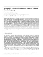
4Learning Vehicle Predictions
To overcome the difficulties associated with creating vehicle and terrain models
for acomplexenvironment that may be unknown or changing, alearning method
is proposed. At the highest level, this approach is about closing the loop around
vehicle predictions, as shown in figure 2. Avehicle prediction is amapping from
environmental sensor information and current vehicle state to future vehicle motion.
This mapping is learned by observing actual vehicle motion after driving overa
giventerrain. During training and execution, the vehicle makes predictions about
the future state of the vehicle by reasoning about its current state and the terrain in
front of the vehicle. Then, when the vehicle drivesoverthat terrain, it compares its
predictions to what actually happened. This feedback is used for continual learning
and adaptation to the current conditions.
By closing the loop around vehicle predictions and improving the system models
on-line, tuning asystem to agiven application is easier,the system can handle
changing or unknown terrain, and the system is able to improve its performance over
time.
The learning vehicle predictions approach has been applied to the problem of
finding the load-bearing surface in vegetation. The system makes predictions of the
Learning Predictions of the Load-Bearing Surface 87
Time T+NTime T
m
i j
Fig.2. Learning vehicle predictions. Features from map cell m
ij
extracted at time T are used
to makeaprediction. Then, at time T + N the vehicle traverses the area and determines if its
prediction is correct. This feedback is used to improve the model.
load-bearing surface from features extracted from the laser range points. Then it
drivesoverthe terrain and measures the true surface height with the rear wheels.
These input-output pairs are used as training examples to alocally weighted learner
that learns the mapping from terrain features to load-bearing surface height. Once the
load-bearing surface is known, parameters of interest such as roll, pitch, clearance,
and suspension limits can easily be computed using akinematic vehicle model as
described in section 3.
This combination of kinematic equations with machine learning techniques offers
several advantages. Known kinematic relationships do not need to be learned, so the
learner can focus on the difficult unknown relationships. Also, the learned function
can be trained on flat safe areas, butisvalid on steep dangerous areas. If we learned
the roll and pitch directly,wewould need to provide training examples in dangerous
areas to get valid predictions there.
4.1 FeatureExtraction
As described in section 2, the range points from the ladars are collected overtime
in aworld frame grid. In addition to maintaining the average and lowest height of
points in each cell, we use an approach similar to [3] to takeadvantage of the added
information about free space that alaser ray provides. We maintain ascrolling map
of 3D voxels around the vehicle that records the locations of anyhits in avoxel, as
well as the number of laser rays that pass through the voxel. Each voxelis50cm
square by 10cm tall. We use acell size of 50cm because that is the width of the rear
tires on our tractor,which are used for finding the true ground height.
Four different features are extracted from each column of voxels in the terrain
map. The average height of range points works well for hard surfaces such as roads
and rocks. The lowest point may provide more information about the ground height
if there is sparse vegetation. Vo xels that have ahigh ratio of hits to pass-throughs
are likely to represent solid objects, so the average of the points in these voxels may
help determine the load-bearing surface. As shown in figure 4, the standard deviation
from aplane fit provides agood measure of how“smooth” an area is, and works well
as adiscriminator between hard things likeroad and compressible things likeweeds.
We are currently working on other features that use color and texture information in
addition to laser range points.