Rapid Learning in Robotics - Jorg Walter Part 8 ppt
Bạn đang xem bản rút gọn của tài liệu. Xem và tải ngay bản đầy đủ của tài liệu tại đây (343.22 KB, 16 trang )
7.2 Sensor Fusion and 3 D Object Pose Identification 99
Figure 7.3: Six Reconstruction Examples. Dotted lines indicate the test cube as
seen by a camera. Asterisks mark the positions of the four corner points used as
inputs for reconstruction of the object pose by a PSOM. The full lines indicate the
reconstructed and completed object.
(inter-sensor coordination). The lower part of the table shows the results
when only four points are found and the missing locations are predicted.
Only the appropriate in the projection matrix (Eq. 4.7) are set to one,
in order to find the best-matching solution in the attractor manifold. For
several example situations, Fig. 7.3 depicts the completed cubical object on
the basis of the found four points (asterisk marked = input to the PSOM),
and for comparative reasons the true target cube with dashed lines (case
PSOM with ranges 150 ,2 ). In Sec. 9.3.1 we will return to this
problem.
7.2.2 Noise Rejection by Sensor Fusion
The PSOM best-match search mechanism (Eq. 4.4) performs an automatic
minimization in the least-square sense. Therefore, the PSOM offers a very
natural way of fusing redundant sensory information in order to improve the
reconstruction accuracy in case of input noise.
In order to investigate this capability we added Gaussian noise to the
virtual sensor values and determined the resulting average orientation de-
100 Application Examples in the Vision Domain
PSOM range
4 and 8 points are input
150 2 2.6 3.1 2.9 0.11 0.039 0.046 0.0084 given given
150 2 2.7 3.2 2.8 0.12 0.043 0.048 0.0084 0.010 0.0081
Learn only rotational part
3 3 3 150 2.6 3.0 2.5 0.046 0.048 0.0074 0.018 0.012
4 4 4 150 0.63 1.2 0.93 0.021 0.019 0.0027 0.013 0.0063
5 5 5 150 0.12 0.12 0.094 0.0034 0.0027 0.00042 0.0017 0.00089
Various rotational ranges
90 1 0.64 0.56 0.53 0.034 0.0085 0.0082 0.00082 0.0036 0.0021
120 1 1.5 1.5 1.4 0.037 0.021 0.021 0.0032 0.0079 0.0049
150 1 2.7 3.2 2.8 0.077 0.044 0.048 0.0084 0.013 0.010
180 1 6.5 5.4 7.0 0.19 0.079 0.098 0.014 0.019 0.016
Various training set sizes
150 2 2.7 3.2 2.8 0.12 0.043 0.048 0.0084 0.010 0.0081
150 2 2.6 3.2 2.8 0.11 0.043 0.048 0.0084 0.0097 0.0077
150 2 0.49 0.97 0.73 0.12 0.018 0.016 0.0030 0.0089 0.0059
150 2 0.52 0.98 0.71 0.035 0.017 0.014 0.0026 0.0082 0.0053
150 2 0.14 0.13 0.14 0.024 0.0033 0.0030 0.00043 0.0018 0.0011
Shift depth range
150 1 3 3.8 3.4 3.7 0.12 0.061 0.064 0.0083 0.049 0.025
150 2 4 2.6 3.2 2.8 0.11 0.043 0.048 0.0084 0.0097 0.0077
150 3 5 2.6 3.2 2.9 0.15 0.042 0.047 0.0084 0.0050 0.0045
Various distance ranges
150 2 2.6 3.2 2.8 0.11 0.043 0.048 0.0084 0.0097 0.0077
150 4 2.6 3.2 2.8 0.20 0.042 0.047 0.0084 0.0068 0.0059
150 6 2.6 3.2 2.9 0.36 0.043 0.048 0.0084 0.0057 0.0052
150 6 0.65 0.73 0.93 0.39 0.016 0.013 0.00047 0.0070 0.0051
150 6 0.44 0.43 0.60 0.14 0.0097 0.0083 0.00042 0.0043 0.0029
Table 7.1: Mean Euclidean deviation of the reconstructed pitch, roll, yaw angles
, the depth , the column vectors of the rotation matrix , the scalar
product of the vectors
(orthogonality check), and the predicted image position
of the object locations
. The results are obtained for various experimental
parameters in order to give some insight into their impact on the achievable re-
construction accuracy. The PSOM training set size is indicated in the first column,
the
intervals are centered around 0 , and depth ranges from ,
where
denotes the cube length (focal length of the lens is also taken as .)
In the first row all corner locations are inputs. All remaining results are obtained
using only four (non-coplanar) points as inputs.
7.2 Sensor Fusion and 3 D Object Pose Identification 101
viation (norm in ) as function of the noise level and the number of
sensors contributing to the desired output.
0
5
10
3
4
5
6
7
8
10
15
20
25
<∆(θ,Ψ,Φ)>
Noise [%]
Number of Inputs
Figure 7.4: The reconstruction deviation versus the number of fused sensory
inputs and the percentage of Gaussian noise added. By increasing the number of
fused sensory inputs the performance of the reconstruction can be improved. The
significance of this feature grows with the given noise level.
Fig. 7.4 exposes the results. Drawn is the mean norm of the orientation
angle deviation for varying added noise level from 0 to 10 % of the av-
erage image size, and for 3,4, and 8 fused sensory inputs, which were
taken into account. We clearly find with higher noise levels there is a grow-
ing benefit from an increasing increased number of contributing sensors.
And as one expects from a sensor fusion process, the overall precision
of the entire system is improved in the presence of noise. Remarkable
is how naturally the PSOM associative completion mechanism allows to
include available sensory information. Different feature sensors can also
be relatively weighted according to their overall accuracy as well as their
estimated confidence in the particular perceptual setting.
102 Application Examples in the Vision Domain
7.3 Low Level Vision Domain: a Finger Tip Lo-
cation Finder
So far, we have been investigating PSOMs for learning tasks in the context
of well pre-processed data representing clearly defined values and quanti-
ties. In the vision domain, those values are results of low level processing
stages where one deals with extremely high-dimensional data. In many
cases, it is doubtful to what extent smoothness assumptions are valid at
all.
Still, there are many situations in which one would like to compute
from an image some low-dimensional parameter vector, such as a set of
parameters describing location, orientation or shape of an object, or prop-
erties of the ambient illumination etc. If the image conditions are suitably
restricted, the input images may be samples that are represented as vec-
tors in a very high dimensional vector space, but that are concentrated on
a much lower dimensional sub-manifold, the dimensionality of which is
given by the independently varying parameters of the image ensemble.
A frequently occurring task of this kind is to identify and mark a par-
ticular part of an object in an image, as we already met in the previous
example for determination of the cube corners. For further example, in
face recognition it is important to identify the locations of salient facial
features, such as eyes or the tip of the nose. Another interesting task is to
identify the location of the limb joints of humans for analysis of body ges-
tures. In the following, we want to report from a third application domain,
the identification of finger tip locations in images of human hands (Walter
and Ritter 1996d). This would constitute a useful preprocessing step for
inferring 3 D-hand postures from images, and could help to enhance the
accuracy and robustness of other, more direct approaches to this task that
are based on LLM-networks (Meyering and Ritter 1992).
For the results reported here, we used a restricted ensemble of hand
postures. The main degree of freedom of a hand is its degree of “closure”.
Therefore, for the initial experiments we worked with an image set com-
prising grips in which all fingers are flexed by about the same amount,
varying from fully flexed to fully extended. In addition, we consider ro-
tation of the hand about its arm axis. These two basic degrees of freedom
yield a two-dimensional image ensemble (i.e., for the dimension of the
map manifold we have ). The objective is to construct a PSOM that
7.3 Low Level Vision Domain: a Finger Tip Location Finder 103
Figure 7.5: Left,(a): Typical input image. Upper Right,(b): after thresholding and
binarization. Lower Right,(c): position of
array of Gaussian masks (the dis-
played width is the actual width reduced by a factor of four in order to better
depict the position arrangement)
maps a monocular image from this ensemble to the 2 D-position of the
index finger tip in the image.
In order to have reproducible conditions, the images were generated
with the aid of an adjustable wooden hand replica in front of a black back-
ground (for the required segmentation to achieve such condition for more
realistic backgrounds, see e.g. Kummert et al. 1993a; Kummert et al.
1993b). A typical image ( pixel resolution) is shown in Fig. 7.5a.
From the monochrome pixel image, we generated a 9-dimensional feature
vector first by thresholding and binarizing the pixel values (threshold =
20, 8-bit intensity values), and then by computing as image features the
scalar product of the resulting binarized images (shown in Fig. 7.5b) with
a grid of 9 Gaussians at the vertices of a lattice centered on the hand
(Fig. 7.5c). The choice of this preprocessing method is partly heuristically
motivated (the binarization makes the feature vector more insensitive to
variations of the illumination), and partly based on good results achieved
with a similar method in the context of the recognition of hand postures
104 Application Examples in the Vision Domain
(Kummert et al. 1993b).
To apply the PSOM-approach to this task requires a set of labeled train-
ing data (i.e., images with known 2 D-index finger tip coordinates) that
result from sampling the parameter space of the continuous image ensem-
ble on a 2 D-lattice. In the present case, we chose the subset of images
obtained when viewing each of four discrete hand postures (fully closed,
fully opened and two intermediate postures) from one of seven view direc-
tions (corresponding to rotations in
-steps about the arm axis) spanning
the full -range. This yields the very manageable number of 28 images
in total, for which the location of the index finger tip was identified and
marked by a human observer.
Ideally, the dependency of the - and -coordinates of the finger tip
should be smooth functions of the resulting 9 image features. For real
images, various sources of noise (surface inhomogeneities, small specular
reflections, noise in the imaging system, limited accuracy in the labeling
process) lead to considerable deviations from this expectation and make
the corresponding interpolation task for the network much harder than it
would be if the expectation of smoothness were fulfilled. Although the
thresholding and the subsequent binarization help to reduce the influence
of these effects, compared to computing the feature vector directly from
the raw images, the resulting mapping still turns out to be very noisy. To
give an impression of the degree of noise, Fig. 7.7 shows the dependence
of horizontal ( -) finger tip location (plotted vertically) on two elements of
the 9 D-feature vector (plotted in the horizontal plane). The resulting
mesh surface is a projection of the full 2 D-map-manifold that is embedded
in the space , which here is of dimensionality 11 (nine dimensional input
features space , and a two dimensional output space for
position.) As can be seen, the underlying “surface” does not appear very
smooth and is disrupted by considerable “wrinkles”.
To construct the PSOM, we used a subset 16 images of the image en-
semble by keeping the images seen from the two view directions at the
ends ( ) of the full orientation range, plus the eight pictures belonging
to view directions of . For subsequent testing, we used the 12 images
from the remaining three view directions of and . I.e., both train-
ing and testing ensembles consisted of image views that were multiples of
apart, and the directions of the test images are midway between the
directions of the training images.
7.3 Low Level Vision Domain: a Finger Tip Location Finder 105
Figure 7.6: Some examples of hand images with correct (cross-mark) and pre-
dicted (plus-mark) finger tip positions. Upper left image shows average case, the
remaining three pictures show the three worst cases in the test set. The NRMS
positioning error for the marker point was 0.11 for horizontal, 0.23 for vertical
position coordinate.
Even with the very small training set of only 16 images, the resulting
PSOM achieved a NRMS-error of 0.11 for the -coordinate, and of for
the -coordinate of the finger tip position (corresponding to absolute RMS-
errors of about 2.0 and 2.4 pixels in the image, respectively). To give
a visual impression of this accuracy, Fig. 7.6 shows the correct (cross mark)
and the predicted (plus mark) finger tip positions for a typical average
case (upper left image), together with the three worst cases in the test set
(remaining images).
106 Application Examples in the Vision Domain
Figure 7.7: Dependence of vertical index finger position on two of the nine input
features, illustrating the very limited degree of smoothness of the mapping from
feature to position space.
This closes here the list of presented PSOM applications homing purely
in the vision domain. In the next two chapters sensorimotor transforma-
tion will be presented, where vision will again play a role as sensory part.
Chapter 8
Application Examples in the
Robotics Domain
As pointed out before in the introduction, in the robotic domain the avail-
ability of sensorimotor transformations are a crucial issue. In particular,
the kinematic relations are of fundamental character. They usually describe
the relationship between joint, and actuator coordinates, and the position
in one, or several particular Cartesian reference frames.
Furthermore, the effort spent to obtain and adapt these mappings plays
an important role. Several thousand training steps, as required by many
former learning schemes, do impair the practical usage of learning meth-
ods in the domain of robotics. Here the wear-and-tear, but especially the
needed time to acquire the training data must be taken into account.
Here, the PSOM algorithm appears as a very suitable learning approach,
which requires only a small number of training data in order to achieve a
very high accuracy in continuous, smooth, and high-dimensional map-
pings.
8.1 Robot Finger Kinematics
In section 2.2 we described the TUM robot hand, which is built of several
identical finger modules. To employ this (or a similar dextrous) robot hand
for manipulation tasks requires to solve the forward and inverse kine-
matics problem for the hand finger. The TUM mechanical design allows
roughly the mobility of the human index finger. Here, a cardanic base joint
J. Walter “Rapid Learning in Robotics” 107
108 Application Examples in the Robotics Domain
(2 DOF) offers sidewards gyring of and full adduction with two addi-
tional coupled joints (one further DOF). Fig. 8.1 illustrates the workspace
with a stroboscopic image.
(a)
(b) (c
)
(d
)
Figure 8.1: a–d: (a) stroboscopic image of one finger in a sequence of extreme
joint positions.
(b–d) Several perspectives of the workspace envelope
, tracing out a cubical
10
10 10 grid in the joint space . The arrow marks the fully adducted posi-
tion, where one edge contracts to a tiny line.
For the kinematics in the case of our finger, there are several coordi-
nate systems of interest, e.g. the joint angles, the cylinder piston positions,
one or more finger tip coordinates, as well as further configuration depen-
dent quantities, such as the Jacobian matrices for force / moment trans-
formations. All of these quantities can be simultaneously treated in one
single common PSOM; here we demonstrate only the most difficult part,
the classical inverse kinematics. When moving the three joints on a cubical
10 10 10 grid within their maximal configuration space, the fingertip (or
more precisely the mount point) will trace out the “banana” shaped grid
displayed in Fig. 8.1 (confirm the workspace with your finger!) Obviously,
8.1 Robot Finger Kinematics 109
the underlying transformation is highly non-linear and exhibits a point-
singularity in the vicinity of the “banana tip”. Since an analytical solution
to the inverse kinematic problem was not derived yet, this problem was
a particular challenging task for the PSOM approach (Walter and Ritter
1995).
We studied several PSOM architectures with n
n n nine dimensional
data tuples ( ), where denotes the joint angles, the piston displace-
ment and the Cartesian finger point position, all equidistantly sampled
in . Fig. 8.2a–b depicts a and an projection of the smallest training set,
.
To visualize the inverse kinematics ability, we require the PSOM to
back-transform a set of workspace points of known arrangement (by spec-
ifying as input sub-space). In particular, the workspace filling “banana”
set of Fig. 8.1 should yield a rectangular grid of . Fig. 8.2c–e displays the
actual result. The distortions look much more significant in the joint angle
space (a), and the piston stoke space (b), than in the corresponding world
coordinate result (b) after back-transforming the PSOM angle output.
The reason is the peculiar structure; e.g. in areas close to the tip a certain
angle error corresponds to a smaller Cartesian deviation than in other ar-
eas.
When measuring the mean Cartesian deviation we get an already sat-
isfying result of 1.6 mm or 1.0 % of the maximum workspace length of
160 mm. In view of the extremely small training set displayed in Fig. 8.2a–
b this appears to be a quite remarkable result.
Nevertheless, the result can be further improved by supplying more
training points as shown in the asterisk marked curve in Fig. 8.3. The
effective inverse kinematic accuracy is plotted versus the number of train-
ing nodes per axes, using a set of 500 randomly (in uniformly) sampled
positions.
For comparison we employed the “plain-vanilla” MLP with one and
two hidden layers (units with tanh( ) squashing function) and linear units
in the output layer. The encoding was similar to the PSOM case: the
plain angles as inputs augmented by a constant bias of one (Fig.3.1). We
found that this class of problems appears to be very hard for the standard
MLP network, at least without more sophisticated learning rules than the
standard back-propagation gradient descent. Even for larger training set
sizes, we did not succeed in training them to a performance comparable
110 Application Examples in the Robotics Domain
X
θ
X
r
X
c
X’
r
X
θ
(a) (b)
(c)
+
(d) (e)
Figure 8.2: a–b and c–e; Training data set of 27 nine-dimensional points in for
the 3
3 3 PSOM, shown as perspective surface projections of the (a) joint angle
and (b) the corresponding Cartesian sub space. Following the lines connecting
the training samples allows one to verify that the “banana” really possesses a
cubical topology. (c–e) Inverse kinematic result using the grid test set displayed
in Fig. 8.1. (c) projection of the joint angle space
(transparent); (d) the stroke
position space
; (e) the Cartesian space , after back-transformation.
8.1 Robot Finger Kinematics 111
0.01
0.1
1
10
1086543
Mean Cartesian Deviation [mm]
Knot Points per Axes
2x2x2 used
3x3x3 used
4x4x4 used
Chebyshev spaced, full set
equidistand spaced, full set
0
0.5
1
1.5
2
2.5
3
3.5
4
4.5
1086543
Mean Cartesian Deviation [mm]
Knot Points per Axes
2x2x2 used
3x3x3 used
4x4x4 used
Chebyshev spaced, full set
equidistand spaced, full set
Figure 8.3: a–b: Mean Cartesian inverse kinematics error (in mm) of the pre-
sented PSOM types versus number of training nodes per axes (using a test set
of 500 randomly chosen positions; (a) linear and (b) log plot). Note, the result
of Fig. 8.2c–e corresponds to the smallest training set
. The maximum
workspace length is 160 mm.
to the PSOM network. Table 8.1 shows the result of two of the best MLP-
networks compared to the PSOM.
Network
MLP 3–50–3 0.02 0.004 0.72 0.57 0.54
MLP 3–100–3 0.01 0.002
0.86 0.64 0.51
PSOM
0.062 0.037 0.004
Table 8.1: Normalized root mean square error (NRMS) of the inverse kinematic
mapping task
computed as the resulting Cartesian deviation from the goal
position. For a training set of n
n n points, obtained by the two best performing
standard MLP networks (out of 12 different architectures, with various (linear
decreasing) step size parameter schedules
) 100000 steepest gradient
descent steps were performed for the MLP and one pass through the data set for
PSOM network.
Why does the PSOM perform more that an order of magnitude better
than the back-propagation algorithm? Fig. 8.4 shows the 27 training data
pairs in the Cartesian input space . One can recognize some zig-zig clus-
ters, but not much more. If neighboring nodes are connected by lines, it
is easy to recognize the coarse “banana” shaped structure which was suc-
cessfully generalized to the desired workspace grid (Fig.8.2). The PSOM
112 Application Examples in the Robotics Domain
-40
-30
-20
-10
0
10
20
30
40
-40
-30
-20
-10
0
10
20
3
0
90
100
110
120
130
140
150
160
x
y
z
r
θ
Figure 8.4: The 27 training data vectors for the Back-propagation networks: (left)
in the input space
and (right) the corresponding target output values .
gets the same data-pairs as training vectors — but additionally, it obtains
the assignment to the node location in the 3 3 3 node grid illustrated
in Fig. 8.5.
As explained before in Sec. 5, specifying introduces topological
order between the training vectors . This allows the PSOM to advanta-
geously draw extra curvature information from the data set — information,
that is not available with other techniques, such as the MLP or the RBF
network approach. The visual comparison of the two viewgraphs demon-
strates the essential value of the added structural information.
8.2 A Higher Dimensional Mapping:
The 6-DOF Inverse Puma Kinematics
To demonstrate the capabilities of the PSOM approach in a higher dimen-
sional mapping domain, we apply the PSOM to construct an approxima-
tion to the kinematics of the Puma 560 robot arm with six degrees of free-
dom. As embedding space we first use the 15-dimensional space
spanned by the variables
8.2 The Inverse 6 D Robot Kinematics Mapping 113
-40
-30
-20
-10
0
10
20
30
40
-40
-30
-20
-10
0
10
20
30
90
100
110
120
130
140
150
160
x
y
z
r
s
1
s
2
A∈S
w
a
a
θ
Figure 8.5: The same 27 training data vectors (cmp. Fig. 8.4) for the bi-directional
PSOM mapping: (left) in the Cartesian space
, (middle) the corresponding joint
angle space
. (Right:) The corresponding node locations in the param-
eter manifold
. Neighboring nodes are connected by lines, which reveals now
the “banana” structure on the left.
Here, denote the joint angles, is the Cartesian position of the end
effector of length in world coordinates. and denote the normalized
approach vector and the vector normal to the hand plane. The last nine
components vectors are part of the homogeneous coordinate transforma-
tion matrix
(8.1)
(The missing second matrix column is the cross product of the normal-
ized orientation vectors and and therefore bears no further informa-
tion, see Fig. 8.6 and e.g. (Fu et al. 1987; Paul 1981).)
In this space, we must construct the dimensional embedding
manifold that represents the configuration manifold of the robot. With
three nodes per axis direction we require reference vectors
. The distribution of these vectors might have been found with a SOM,
however, for the present demonstration we generated the values for the
by augmenting 729 joint angle vectors on a rectangular 3 3 3 3 3 3
grid in joint angle space with the missing –
114 Application Examples in the Robotics Domain
θ
θ
θ
θ
θ
θ
l
z
n
o
a
r
Figure 8.6: The 15 com-
ponents of the training data
vectors for the PSOM net-
works: The six Puma axes
and the position
and orien-
tation vectors
, , and of
the tool frame.
components, using the forward kinematics transform equations (Paul 1981)
( [-135 ,-45 ], [-180 ,-100 ], [-35 ,55 ], [-45 ,45 ], [-90 ,0 ],
[45 ,135 ], and tool length ={0,200} mm in direction of the frame,
see Fig. 8.6.
Similar to the previous example, we then test the PSOM based on the
points in the inverse mapping direction. To this end, we specify Cartesian
goal positions and orientation values at 200 randomly chosen inter-
mediate test points and use the PSOM to obtain the missing joint angles .
Thus, nine dimensions of the embedding space are selected as in-
put sub-space. The three components are given in length units
([mm] or [m]) and span intervals of range {1.5, 1.2, 1.6} meters for the given
training set, in contrast to the other six dimensionless orientation compo-
nents, which vary in the interval [-1,+1]. Here the question arises what to
do with these incommensurable components of different unit and magni-
tude? The answer is to account for this in the distance metric . The
best solution is to weight each component in Eq. 4.7 reciprocally to the
measurement variance
var (8.2)
If the number of measurements is small, as it is usual for small data sets,