Recent Advances in Mechatronics - Ryszard Jabonski et al (Eds) Episode 1 Part 4 doc
Bạn đang xem bản rút gọn của tài liệu. Xem và tải ngay bản đầy đủ của tài liệu tại đây (2.56 MB, 40 trang )
3. Maze storing
One of the more useful properties of the maze is its size. For a full
sized maze, we would have 16 rows by 16 columns = 256 cell values.
Therefore we would need 256 bytes to store the distance values for a com-
plete maze. A single byte can be used to indicate the presence or absence
of a wall in the maze. The first 4 bits can represent the walls. A typical cell
byte can look like this:
Bit No. 7 6 5 4 3 2 1 0
Wall W S E N
When we are using the binary bit value for each wall position, we
have North = 1, East = 2, South = 4 and West = 8. Now any combination
of walls in a cell can be represented by a number in the range 0 to 15. For
example if some cell have wall on the West and on the East then this cell
can be represent by value 10 which is 0x0A in hex or 00001010 in binary.
Figure 3: Example of maze storing
Every interior wall is shared by two cells so when we update the
wall value for one cell then we have to update the wall value for its
neighbor too.
4. The Flood-fill algorithm
The idea of flood-fill algorithm is to start at the goal (centre of the
maze) and fill the maze with values which represent the distance from each
cell to the goal. When the flooding reaches the starting cell then we can
stop and follow the values downhill to the goal. In the figure 4 we can see
the sequence of the maze being flooded. This maze is completely mapped
and we know where all walls are. We can clearly see how dead ends are
handled and what happens when there is more than one way through maze.
10 T. Marada
Figure 4: Sequence of the maze being flooded
For a full sized maze, we would have 16 rows by 16 columns =
256 cell values. Therefore we would need 256 bytes to store the distance
values for a complete maze. Because the micro-mouse can’t move diago-
nally, the values for a 5x5 maze without walls would look like this:
Figure 5: Flood-Fill example without walls
When it comes time to make a move, the robot must examine all
adjacent cells which are not separated by walls and choose the one with the
lowest distance value. In our example in the figure 5, the robot would ig-
nore any cell to the West because there is a wall, and he would look at the
distance values of the cells to the North, to the East and to the South since
those are not separated by walls. The cell to the North has a value 2, the
cell to the East has a value 2 and the cell to the South has a value 4. That
means that the robot can go to the North or to the East and traverse the
same number of cells on its way to the destination cell. Because turning
would take time, the robot will choose to go forward to the North cell.
When the new walls are found, the distance values of the cells are affected
and we have to update them. Look at the example in the figure 6.
10e robot for practical verifying of articial intelligence methods: Micro-mouse task
Figure 6: Sequence of the regular flood-fill algorithm
In the third step the robot has found a wall. We can’t go to West
and we cannot go to the East, we can only travel to the North or to the
South. But going to the North or to the South means going up in distance
values which we do not want to do. So we need to update the cell values as
a result of finding this new wall. To do this we "flood" the maze with new
values (step fourth). The same case we can see in the seventh step and
eighth step where robot find new wall and distance values had to change.
5. Conclusion
We have implemented regular flood-fill algorithm in to the robot.
This algorithm is very well applicable when the maze includes the single
islands. The flood-fill algorithm is a good way of finding the path from the
start cell to the destination cells, but he is very slow.
Acknowledgements
This work was support by project MSM 0021630518 "Simulation
modeling of Mechatronics systems".
References
[1] Marada T., Houška P., Paseka T.: Small autonomous robot for practical
verifying of artificial intelligence methods, Engineering mechanics 2006,
Svratka 2006.
106 T. Marada
The enhancement of PCSM method by motion
history analysis.
S. Věchet, J. Krejsa, P. Houška
Brno University of Technology, Faculty of Mechanical Engineering,
Technická 2, 616 69, Brno, Czech Republic
Abstract
This paper deals with the identification of wheel robot position and orien-
tation when dealing with the global localization problem. We used a me-
thod called PCSM (Pre-Computed Scan Matching) for solving this prob-
lem for autonomous robot in known environment. This method was devel-
oped for small robots. The identification of the position and orientation of
the robot is based on the fusion of pre-computed match data and the analy-
sis of the history of robot motion. The paper provides information about
this fast yet simple method.
1. Introduction
Navigation of mobile robots is an actual problem in robotics. Many suc-
cessful applications of mobile robots contribute to the further expansion of
robots to the ordinary life. Rescue, survey or delivery robots in dangerous
environment are standard applications.
Identification of robots position relative to the environment is basic task in
navigation. This problem is called localization. Mobile robots localization
is divided into three main parts: the first and simplest is the position track-
ing, the second is local localization (the initial position of the robot is
known) and the last and the most complicated is the global localization
(the initial position of the robot is unknown). Pre-Computed Scan Match-
ing method (PCSM) is presented in this paper. The method was introduced
in [1]. PCSM method belongs to the group of global localization methods.
Presented method solves among other a robot kidnapped problem, when
the robot is taken (kidnapped) from correctly localized position to another
position without any information about the position change.
PCSM method is designed mainly to solve a robot kidnapping problem
with no respect to previous localization results. The method itself is fast
and highly efficient, it failed only in couple of cases. When the localization
fails, the position of the robot is found in totally different position and his-
tory analysis of robot motion can be incorporated to correct the true posi-
tion of the robot in a fast and simple way.
2. Localization method
PCSM (Pre-computed Scan Matching) algorithm was first described in [1].
The algorithm is based on pre-computed world scans and matching of the
scans with actual neighborhood scan. The key idea is to define a value
function used to describe the difference between two scans over the state
space. This is typically called the “Match” and is denoted as
(
)
( ) , ,
M x r x a S
=
(1)
where x is the state (robot pose), a denotes the actual perceptual data read-
ing by robot in given state (such as infrared sensor measurements), S
represents a set of m samples distributed uniformly in state space, r is a
reward function which returns the „match“ for given inputs x,a,S.
The match is computed for each sample as follows:
Let’s assume the robot's pose is x, and let o denote the individual sensor
beam with skew
relative to the robot then the distance d read for this
beam is given according to
( , )
j j
d g x o
=
(2)
( , )
j
g x o
denotes the measurement of an ideal sensor
{
}
1, ,
j
j n
d d
=
=
(3)
then the set S of m samples is
( ) ( )
{
}
1, ,
,
i i
i m
S x d
=
=
(4)
and the reward function r is
( )
( )
( )
( )
2
0
, ,
n
i i
j i
j
r x a S d a
=
= −
∑
(5)
10 S. Vĕchet, J. Krejsa, P. Houška
3. History analysis
Presented method was tested in static environment with known map. The
aim of the method is to successfully identify robot correct position in
known map from neighborhood scans and odometry.
During the beginning of the localization process the robots position in the
map is unknown. When the robot gets the first neighborhood scan, the lo-
calization method identifies a number of possible locations (see figure 1).
Fig. 1: possible location for the robot
Each location is defined as position and orientation
[
]
T
P x y
ϕ
=
and
the localization method produces a set of probable locations
{
}
0 01 02 0
, , ,
n
S P P P
=
. When the robot performs a single movement in
given direction the neighborhood scan is changed and the localization me-
thod produces another set
{
}
1 11 12 1
, , ,
n
S P P P
=
of possible locations for
the robot. After the movement the robot has also the information about the
traveled distance from odometry. The comparison of probable locations
from both steps S
0
and S
1
with traveled distance result in a restricted set of
possible robots locations (see figure 2). The algorithm works as follows:
1. Initialization of pre-computed scans from know map
2. Get the first range scan of robots neighborhood
{
}
1 2
, , ,
i i i in
S P P P
=
3. Single movement, read the odometry information
10e enhancement of PCSM method by motion history analysis
4. Get the range scan
{
}
1 1,1 1,2 1,
, , ,
i i i i n
S P P P
+ + + +
=
5. Perform a history analysis
6. Continue with step 3
Fig. 2: localization process with history analysis
3. Conclusions
We present a localization method PCSM for mobile robots. PCSM method
is used for localization in known static environment and was successfully
used in simulation experiments. The method itself failed to localize the
robot in several cases therefore it was improved by motion history analy-
sis. The capability to successful identify robots position is enhanced and
outliers in robot position are eliminated.
This work was supported by Czech Ministry of Education by project
MSM 0021630518 "Simulation modelling of mechatronic systems".
References
[1] Věchet S., Krejsa J. (2005) Real-time localization for mobile robot,
Mechatronics, robotics and biomechanics 2005, pp 3-13.
110 S. Vĕchet, J. Krejsa, P. Houška
Mathematical Model for the Multi-attribute
Control of the air-conditioning in green houses
Wojciech Tarnowski, Prof. Dr. Habilit.
(a)
, Bui Bach Lam, MSc
(b)
(a) (b)
Control Engng Dept
Technical University, Koszalin, 75-620 Poland
Abstract
In the paper an extended model is presented, which includes all substantial
phenomena in the green-house: conversion of mass and energy, and neces-
sary boundary conditions, and a transportation of water and heat between
the air, soil and plants. The mathematical model of partial differential equ-
ations is proposed.
1. Introduction
The effective growth of plants in green-houses requires that many condi-
tions and constraints are to be met, these are: humidity both of the soil and
of the air, as well as the illumination and the temperature and, what more
these requirements are related each to other (see Fig. 1, for example). Be-
sides, values of the requirements are changing in time depending on the
phase of the development of the plant, and are different for various plants
and even for various species [3], [4].
To design the control system and its algorithm, a mathematical model of
the green-house is necessary to determine current data for the control algo-
rithm, to define adequate instrumentation and to complete verification
experiments. For the optimal real time control an efficient numerical mod-
el is compulsory, too.
2. The object
A modern green-house is a complex of many building segments, joint to
create a broad common inner space, usually of hundreds square meters of
the size. On account of the extensiveness of the greenhouse, usually in the
same time in different zones there are planted various plants with different
climate requirements. To achieve these variety, in each section there are
separate heaters, ventilators, sprinklers, humidifiers, and/or folding win-
dows Therefore it is rational technologically and economically to imple-
ment a dispersed control system with a few valves or heaters and with few
independently controlled devices (what is the MIMO system). Also, the
controlled object must be modelled as the space-continuous unit (i.e. with
distributed parameters) in the 3D space.
3. Requirements for the model
Mathematical model is necessary to design the control installation and then
to control the air conditioning process in a real time. So it must be fast
computable for the predictive control, for example. Next, it should be valid
within the operations limits of disturbances and control variables (tempera-
ture 0 – 40
o
C., humidity 50 – 100%, wind velocity 0 – 30 m/s etc) and the
model must deliver an explicit functions of design variables and control
variables: temperature, humidity and velocity.
The model must be valid only for dry air, otherwise - if the condensation
occurs, an emergency control program (with another model) is to be
switched on, because it is very harmful for plants.
Besides, the model must offer an adequate accuracy, for example 1
o
C for
the temperature, 0,1 m/s for the inner air velocity, and 5 % for the air hu-
midity.
For the research purposes the model should be of an analytical, not of an
experimental character [2], [5].
4. Nominal (physical) model
Processes to be described are: mass and heat conversion within the green
house (in the air and with plants) and through the walls, and between the
walls and the ambient air.
Physical phenomena that are to be considered are:
1. heat conversion,
2. water/steam conversion (evaporation and condensation), mass and
heat diffusion and thermo-diffusion flow of the air inside and out-
side of the object, and via folding windows and ventilators,
3. sunshine radiation on the soil and on plants,
4. evaporation of plants and the soil.
Critical assumptions for the model design are:
1.3D model is necessary for modern greenhouses due to their extension
in all dimensions;
2.Air humidity and temperature is off the dew-point (saturation point);
11 W. Tarnowski, B. B. Lam
3.Small drops of the pressure, thus small the air velocity (Mach < 0,3);
4.No internal sources of mass or energy, except heaters, and/or water
sprinklers;
5.The green-house is leak-proof and air-tight.
Simplifications
On the basis of the above assumptions, the following simplifications may
be adopted.
1. Mass and heat diffusion in the inner air is neglected;
2. Air is a viscose, one-phase fluid;
3. Laminar flow of the air;
4. Mass and energy interchange with the outside atmosphere only by
folding windows and ventilators;
5. No heat conduction along the walls;
6. Constant wind outside the green-house.
5. Mathematical model
Symbols
a
-
heat diffusion coefficient (
12 −
sm
);
Srośr
-
planting area (
2
m
);
Sgrz
-
heating surface (
2
m
);
C
-
specific heat of the air (
11 −−
KJkg
);
Cpr
-
specific heat of vaporization (
1−
Jkg
);
d
-
steam diffusion coefficient in
the air(
12 −
sm
);
Is
-
sunshine radiation intensity (
2−
Wm
);
VpVzVyVx ,,,
-
air velocity components & heating water (
1−
ms
);
M
-
absolute air humid-
ity inside the green-house (
1
2
)(
−
kgOHkg
);
Mro
-
steam transpiration
efficiency of plants (
21
2
)(
−−
msOHkg
);
NgrzNro
,
-
binary signal of the
presence of vegetables/heaters;
m
q
- steam evaporation stream
(
21
2
)(
−−
msOHkg
);
R
- gas constant;
T
- air temperature (
K
);
TgrzTro
,
-plants, heater temperature (
K
);
tt
∆
,
- time, step of time (
s
);
z
y
x
,
,
,
zyx
∆
∆
∆
,,
- Space coordinates, step values (
m
)
kji ,,
- indexes
of nods for coordinates ox, oy, oz;
maxmaxmax
,, kji
- end indexes in coordi-
nates ox, oy, oz;
n
-last time step index;
pk ro p w
, , ,
α α α α
-convection heat
coefficients (
12
−−
KWm
);
ρ
- specific material density (
3
−
kgm
);
µ
- dy-
namic viscosity (
12
−
sm
);
ε
- coefficient of the sunshine radiation absorp-
tion;
ϖ
- tilt angle of roof;
ϕ
-angle of the sun light.
11Mathematical model for the multi-attribute control of the air-conditioning in green
The heat and mass conservation equations are [1]:
2
∂ µ ∂ ∂ ∂ ∂
= ⋅ ∇ − ⋅ − ⋅ − ⋅ − ⋅
∂ ρ ∂ ∂ ∂ ∂
Vx Vx Vx Vx T
Vx Vx Vy Vz R
t x y z x
(1)
y
T
R
z
Vy
Vz
y
Vy
Vy
x
Vy
VxVy
t
Vy
∂
∂
⋅−
∂
∂
⋅−
∂
∂
⋅−
∂
∂
⋅−∇⋅=
∂
∂
2
ρ
µ
(2)
z
T
R
z
Vz
Vz
y
Vz
Vy
x
Vz
VxVz
t
Vz
∂
∂
⋅−
∂
∂
⋅−
∂
∂
⋅−
∂
∂
⋅−∇⋅=
∂
∂
2
ρ
µ
(3)
υ
ρ
q
Cz
T
Vz
y
T
Vy
x
T
Vx
t
T
⋅
+
∂
∂
⋅−
∂
∂
⋅−
∂
∂
⋅−=
∂
∂
1
(4)
m
q
z
M
Vz
y
M
Vy
x
M
Vx
t
M
+
∂
∂
⋅−
∂
∂
⋅−
∂
∂
⋅−=
∂
∂
(5)
)(
grzp
m
TTp
x
T
Vp
t
Tp
−⋅+
∂
∂
⋅−=
∂
∂
α
(6)
)()( TTTTp
t
T
grzzgrzw
grz
−⋅−−⋅=
∂
∂
αα
(7)
zyx
MroNroMzwNzw
q
m
∆⋅∆⋅∆
⋅
+
⋅
=
(8)
grz grz grz grz ro ro
pr
Ngrz S (T T) Ngrz S Is cos Nro S (Tro T)
q
x y z
C
T
C t
υ
⋅α ⋅ ⋅ − + ⋅ ⋅ρ⋅ ⋅ ϕ+ ⋅α ⋅ ⋅ −
= −
⋅ ⋅
∂
− ⋅
∂
∆ ∆
(9)
Boundary Conditions
Boundary Conditions (BCs) and Initial Conditions must be defined for
velocity, temperature and humidity. For example BCs for the roof in the
partly incremental form are:
0
=
=
=
VzVyVx
(10)
2 i 1,jkn ijkn i,j 1,kn
2 2 2
ijkn
pk
z
T T T T T
a 2a
t z ( x) ( y)
(T T )
2 cos Is
-
C x C cos x
+ −
∂ ∂ −
= + + −
∂ ∂
α
−
⋅ ε ⋅ ϕ
+ ⋅
ρ ⋅ ρ ⋅ ⋅ ϖ
∆ ∆
∆ ∆
(11)
11 W. Tarnowski, B. B. Lam
∆
−
+
∆
−
+
∂
∂
=
∂
∂
−+
2
,1,
2
,1
2
2
)()(
2
y
MM
x
MM
d
z
M
d
t
M
ijknknjiijknjkni
(12)
6. Digital model
To solve the mathematical model a computer technique is necessary. Gen-
erally, there are two possibilities:
1) to arbitrary mesh the object, elaborate a set of time continuous ordinary
differential equations as incremental equations for discrete space and/or
time variables and to devise a specific user-individual code for the mesh of
final elements;
2) to apply a commercial MES package.
For some practical reasons the first approach was chosen. The model was
converted to a fully incremental form and coded in Visual Basic language
[6]. Graphical user interfaces are devised, also. User may observe results
of computations: the temperature, the humidity and three components of
the velocity in a specific point of the green-house as a function of time.
References
[1] W. Tarnowski, ”Modelowanie systemów” (Modeling of systems in engineer-
ing) Wydawnictwo Uczelniane Politechniki Koszalińskiej (2004)
[2] H. Latała, ”Wpływ zewnętrznych warunków klimatycznych na dynamikę
zmian temperatury i wilgotności powietrza w szklarni” (On the influence of
ambient conditions on the micro-climate in green-houses), Praca doktorska,
(PhD Thesis), Akademia Rolnicza, Kraków (1997)
[3] T. Pudelski ”Uprawa warzyw pod osłonami” Praca zbiorowa. Państwowe
Wydawnictwo Rolnicze i Leśne (1998)
[4] C. Stanghellini, W.Th.M.van Meurs, “Environmental Control of Greenhouse
Crop Transpiration” J. Agric. Eng Res (1992) 51, 297-311
[5] K. Popowski, ”Greenhouse climate factors” Faculty of Technical Science,
Bitola University, Bitola, Macedonia (2004)
[6]. W. Tarnowski, Bui Bach Lam “Computer simulation model of green houses
for the multi-attribute control of the air-conditioning”,
ISSAT International
Conference on Modeling of Complex Systems and Environments July
16-18, 2007 Ho Chi Minh City, Vietnam, 2007.
11Mathematical model for the multi-attribute control of the air-conditioning in green
Kohonen Self-Organizing Map for the Traveling
Salesperson Problem
Łukasz Brocki, Danijel Koržinek
Polish-Japanese Institute of Information Technology,
ul. Koszykowa 86, 02-008, Warsaw
Abstract
This work shows how a modified Kohonen Self-Organizing Map with one
dimensional neighborhood is used to solve the symmetrical Traveling Sa-
lesperson Problem. Solution generated by the Kohonen network is im-
proved using the 2opt algorithm. The paper describes briefly self-
organization in neural networks, 2opt algorithm and modifications applied
to Self-Organizing Map. Finally, the algorithm is compared with the Evo-
lutionary Algorithm with Enhanced Edge Recombination operator and
self-adapting mutation rate.
1. Introduction
The aim of the Traveling Salesperson Problem (TSP) is thus: given a set of
n cities and costs of traveling between all pairs of cities, what is the cheap-
est route that visits each city exactly once and returns to the starting city.
This problem is the leading example of NP-hard problems. Its search space
is exceptionally huge (n!) and given that some engineering problems, like
VLSI design, need as many as 1.2 million cities [5], a fast and effective
heuristic method is desired.
In this paper, we present a neural based algorithm and compare it to an
effective heuristic method: Evolutionary Algorithm with the Enhanced
Edge Recombination operator.
2. Kohonen Self-Organizing Map for the TSP
In 1975, Teuvo Kohonen introduced a new type of neural network that
uses competitive, unsupervised learning [1]. The principle of his algo-
rithm is to adapt a special network to a set of unorganized and unlabeled
data. After the training phase, this network can be used for clustering and
simple classification tasks.
Interesting results of self-organization can be achieved with networks that
have a 2-dimensional input vector and a 1-dimensional neighborhood. In
this case the input to the network can be regarded as coordinates in a 2-
dimensional space: x and y. Using this technique, one can map a line over
an arbitrary binary image. Furthermore, if one provides the algorithm with
the same number of neurons as the number of cities it will output an effi-
cient tour of the cities, as depicted in Figure 1.
Figure 1. Solving a simple TSP problem. The example consists of six squares. The
first one shows an object that is to be learned. The second square illustrates the
network just after the randomization of all neural weights. Following squares illu-
strate the learning process. Please note that each neuron (a circle) represents a
point whose coordinates are equal to the neuron's weights.
3. Modifications
Given a solution, like the one above, two things can be done to further en-
hance the result. First, because the algorithm works by altering the real-
valued weights of the neurons it may never achieve the exact values that
match the coordinates of the cities. A simple procedure was therefore
created to restore the 1-1 mapping between the cities and the individual
neurons.
Another improvement can be achieved by applying the well-known and
fast 2-opt algorithm. This algorithm works by rearranging pairs of paths
connecting the cities in a way that yields a cheaper overall tour. 2-opt pro-
vides locally optimal solutions and when starting from a random arrange-
ment of cities, doesn’t yield a perfect result. However, thanks to its sim-
plicity it is often used in optimizing already good solutions.
4. The Experiment
Two types of tests were administered: using city sets taken from the
TSPLIB [6] and using randomly chosen cities. TSPLIB city sets are quite
11Kohonen self-organizing map for the traveling salesperson problem
difficult. The reason for this is that in many cases cities are not chosen in
random. Often larger city sets consist of smaller patterns. The optimal tour
is therefore identical in each of the smaller patterns. SOM, on the other
hand, tries to figure out a unique tour in each smaller pattern.
Testing using randomly chosen cities is more objective. It is based on the
Held-Karp Traveling Salesman bound [4], which is an empirical relation
between expected tour length, number of cities and the area of square box
on which cities are placed. Three random city sets were used in this expe-
riment (100, 500, 1000 cities). Square box edge length was 500.
All statistics for SOM were generated after 50 runs on each city set. Aver-
age tour lengths for city sets up to 2000 cities are around 5 to 6 percent
worse than the optimum. SOM approach can generate solutions that are
almost always less that 10% worse from the optimal tour. However, in
most cases the difference is just a few percent.
SOM has been compared to EA coupled with the Enhanced Edge Recom-
bination (EER) operator [2, 3], Steady-State survivor selection (where al-
ways the worst solution is replaced), Tournament parent selection with
tournament size depending on number of cities and population size.
Scramble mutation was used. Optimal mutation rate depends on amount of
cities and state of evolution. Therefore, self-adapting mutation rate has
been used. Every genotype has its own mutation rate, which is modified in
a similar way as in Evolution Strategies. This strategy adapts mutation rate
to number of cities and evolution state automatically, so it is not needed to
manually check which parameters are optimal for each city set. Evolution
stops when the population converges. Population size was set to 1000 (as
in [3]). When EA stopped its best solution was optimized by the 2-opt al-
gorithm. Results for both SOM and EA are shown in Table 1.
All statistics for SOM were generated after 50 runs on each city set. For
EA there were 10 runs of the algorithm for sets: EIL51, EIL101 and
RAND100. For other sets EA was run only once. Optimum solutions for
instances taken from TSPLIB were already given and optimum solutions
for random instances were calculated from the empirical relation described
above. All computations were performed on an AMD Athlon 64-bit 3500+
processor.
Self-Organizing Map Evolutionary Algorithm
Instances Optimum Ave.
Result
Best
Result
Ave
Time
Ave
Result
Best
Result
Ave
Time
EIL51 426 444 431 0.068 428.2 426 10
EIL101 629 662 646 0.127 653.3 639 75
TSP225 3916 4192 4106 0.302 4044 871
11 Ł. Brocki, D. Koržinek
Self-Organizing Map Evolutionary Algorithm
Instances Optimum Ave.
Result
Best
Result
Ave
Time
Ave
Result
Best
Result
Ave
Time
PCB442 50778 56634 55138 0.703 55657 10395
PR1002 259045 278481 274036 2.425 286908 25639
PR2392 378037 418739 411442 12.965
RAND100 3851.81 4051 3882 0.131 3931.4 3822 69.6
RAND500 8203.73 8888 8697 0.824 9261 11145
RAND 1000 11475.66 12483 12343 2.311 12858 56456
Table 1. The results of the experiments. Time is given in seconds. First six expe-
riments are from the TSPLIB and the last three are random.
5. Conclusions
It seems that SOM-2opt hybrid is not a very powerful algorithm for the
TSP. It has been outperformed by EA. On the other hand it is much faster.
There are many algorithms that solve permutation problems. Evolutionary
Algorithms have many different operators that work with permutations.
EER is one of the best operators for the TSP [3]. However, it was proved
that other permutation operators, which are worse for the TSP than EER,
are actually better for other permutation problems (like ware-
house/shipping scheduling) [3]. Therefore, it might be possible that SOM-
2opt hybrid might work better for other permutation problems than for the
TSP.
We are grateful to Prof. Zbigniew Michalewicz for influencing and helping
us to write this paper.
References
[1] Kohonen T. (2001), Self-Organizing Maps, Springer, Berlin.
[2] Michalewicz Z. (1996), Genetic Algorithms + DataStructures = Evolution
Programs, Springer – Verlag.
[3] Starkweather T., McDaniel S., Whitley C., Mathias K., Whitley D., (1991), A
Comparison of Genetic Sequencing Operators.
[4] Johnson, D.S., McGeoch, L.A., and Rothberg, E.E., Asymptotic experimental
analysis for the Held-Karp traveling salesman bound.
[5] Korte B., (1988), Applications of Combinatorial Optimization.
[6] Reinelt G., (1995), TSPLIB 95 documentation, University of Heidelberg.
11Kohonen self-organizing map for the traveling salesperson problem
Simulation modeling, optimalization and
stabilisation of biped robot
P. Zezula, D. Vlachý, R. Grepl
Institute of Solid Mechanics, Mechatronics and Biomechanics,
Faculty of Mechanical Engineering, Brno University of Technology, Brno,
Czech Republic
Institute of Thermomechanics, Academy of Sciences of the CR, branch
Brno, Czech Republic
Abstract
This paper deals with proposal of humanoid robot construction. The con-
struction of two legs (six DOF each) is described. Computational model-
ling was used, particularly forward and inverse kinematic model. By help
of these models was produce several functions for the control of moving
robot´s body. Coordination of robot move was simulated in environment
VRML.
Key words: biped robot, computer modeling,
1. Introduction
The scientific field of mobile robotics represents an interesting branch for
the research and development in mechatronics. This topic becomes more
and more actual for the population, because by using of the different ro-
botic manipulators and walking machines the people can make easier a lot
of their work. Also, the development of manipulators bring new knowl-
edge in mechanics, electronics, neural network and others.
In this paper, there is briefly described the design of mechanical construc-
tion biped robot Golem 2, that was built at FME Brno, University of Tech-
nology. There is issue about the stability of robot. The solution of stability
allows the gait on irregular terrain.
we have solved all problem by using computer simulation in MAT-
LAB/Simulink/SimMechanics and visualization of results in VRML.
.
2. Mechanical construction
During the design of mechanical construction we have used a several tools.
First of them is forward kinematic model (FKM). This model can be sym-
bolically described by equation (1).
],,,,,[],,,,,[
zyx
zyx
ϕϕϕξηδγβα
=
(1)
Where
ζ
η
δ
γ
β
α
,,,,,
are angles of joints
x, y, z are cartesian position of foot
zyx
ϕϕϕ
,,
is spatial orientation of foot
Kinematic structure is shown in Fig. 1. The construction has total 12 DOF.
Their disposition is following. In each hip joint, there are placed three
DOF, each knee has one DOF and in area of each ankle are situated two
DOF.
11Simulation modeling, optimalization and stabilisation of biped robot
Fig. 1. Geometry of robot
If we want to obtain new servos position and we know Cartesian position
of foot and spatial orientation of foot we use inverse kinematic model
(IKM), that we can describe by equation (2).
],,,,,[],,,,,[
ξηδγβαϕϕϕ
=
zyx
zyx
(2)
Further information about FKM and IKM is possible to find in [1].
3. Modelling of robot and visualization
The construction has been made true to scale in program system Solid-
Works 2001 after optimalization geometric and mass parameters. So we
have obtained visual image and we were able to observe crash states too.
The final model of construction is shown in Fig. 2.
1 P. Zezula, D. Vlachý, R. Grepl
Fig. 2. Model of robot (left in SolidWorks, right in Matalb)
On base of this model were made some functions in M
ATLAB
. We are able
to coordinate move of robot by help these functions. In following text is
briefly described, how inputs and outputs the functions have.
The inputs are actual positions of servos and new coordinate of body with
respect to global coordinate system O-XYZ. Outputs of functions are new
position of servos. By help of new servo positions we obtain require move
of robot body. Those functions are based on FKM and IKM [1]. Now we
are able to interpolate step between actual and new servos position and
obtained data we used for visualization in VRML.
4. Stability of robot - Criterion ZMP
During the suggestion of the mechanical design, it is necessary to solve the
stability problem of the robot. There is no unique definition of the problem
for biped balance control. There are many position, which can become un-
stable and the robot can fall down. We can solve this problem by the using
of workspace and we search through this workspace for stable states of
robot. The criterion zero moment point (ZMP) is usually used. This point
has to lie in supporting area of foot, when the robot stands on one leg or in
supporting area of feet and between the feet, when robot stands on two leg.
It means that we have to know position of YMP with respect 0-XYZ in
every moment during walk.
1Simulation modeling, optimalization and stabilisation of biped robot
Fig. 3. Experiment
We have solved this problem by using the M
ATLAB
environment, where
we created the algorithm of computing ZMP. With help of statical model
(Fig.2) we obtain contact forces between foot and ground. This contact
forces have to remain of compression character and it means, that the posi-
tion is stable. We measure those forces in area of tee, little toe and heel.
Next we compute the actual position of ZMP from obtaining forces. This
actual coordinate of ZMP is compared with required coordinated of ZMP.
Required coordinates of ZMP are referred to local 0-XYZ, which is con-
nected with ankle. We used the actual of ZMP as input to function, which
calculate new position of servos. This function contains analytical inverse
kinematic model of robot.
In program M
ATLAB
/Simulink/SimMechanics we define a position, which
is stable. Then we demonstrated this position on real construction of robot
and we were able to verify the numerical results. The described experiment
is shown in Fig. 3.
1 P. Zezula, D. Vlachý, R. Grepl
4. Conclusion
The most important tools for coordination move of robot FKM and IKM
have been created in program MAPLE. For verification of FKM and IKM
we used M
ATLAB
/Simulink/SimMechanics and sequentially VRML.
Acknowledgment
The published results have been acquired be support of project
AV0Z20760514 and GA�R 101/06/0063.
References
[1] R. Grepl, P. Zezula, “Modelling of kinematics of biped robot”, Collo-
quium Dynamics of Machines 2006, Prague, February 7-8, Czech Repub-
lic, ISBN 80-85918-97-8, 2006
[2] Ch.Zhou, Q. Meng, “dynamic balance of a biped robot using fuzzy re-
inforcement learning agents”, 2005
[3] Y. Tagawa, T. Yamashita, “Analysis of human abnormal walking using
zero moment joint”, 2000
1Simulation modeling, optimalization and stabilisation of biped robot
Extended kinematics
for control of quadruped robot
R.Grepl
Institute of Solid Mechanics, Mechatronics and Biomechanics,
Faculty of Mechanical Engineering, Brno University of Technology,
Czech Republic,
Abstract
This paper deals with the extended kinematical model for quadruped mo-
bile walking robot. The model has been built based on homogenous coor-
dinates approach. The robot is comprehended as an open tree manipulator
and therefore standard algorithms for forward and inverse kinematics can
be employed. However, the inverse model named 12-18 works with the
redundant manipulator structure and pseudoiverse of Jacobian matrix
should be used. The inverse model 3-3 uses regular manipulator and al-
lows separate positioning of each leg. After processing and simplification
of the equations in Maple, the algorithms have been implemented in Mat-
lab environment. The model automatically built in SimMechanics has been
used for verification. Finally, the results have been tested using VRML
visualization.
1. Introduction
This paper describes briefly the extended kinematical model for quadruped
walking robot based on homogenous coordinates. The work is aimed to
particular project of robot Jaromír (Fig. 1) built at FME Brno University of
Technology. Robot has in total 12 controlled servo drives, further details
has been published in [2].
The control algorithms for irregular terrain as well as advanced gait and
movement controllers inevitably require the 6D control of the robot body.
Simple models designed relatively to body c.s. can be hardly used for such
a task.
In following text, the forward and two inverse kinematical models are in-
troduced as well as a few notes about visualization in VRML.
Fig. 1. Four legged robot Jaromír during its regular walk
2. Forward kinematical model (FKM)
The FKM positions and orients the body and all four legs of the robot rela-
tively to global coordinate system. So, the robot is understood as an open
tree manipulator with four end effectors P. Forward kinematics of all legs
can be apparently separated to individual ones, and described by parame-
ters
, , , , , , , ,
T T T
x y z
ϕ ϑ ψ α β γ
:
1 1 1
3
= [ , , ] =
= [ ,0,0,1]
( , , , , , , , , ) =
P P P
T
T T T
x y z
L
x y z
ϕ ϑ ψ α β γ
P P
1 81 8
P
8
81 21 32 87
r T r
r
T T T T
(1)
where r
1
P
is the position of end of robotic leg in global c.s. 1, r
8
P
in leg
c.s. 8. Matrix T
81
incorporates the homogenous transformation between
those two systems and depends on position x
T,
y
T,
z
T
and orientation (Euler
angles
, ,
ϕ ϑ ψ
in RPY notation) of the body and three angles of leg servo
drives
, ,
α β γ
. Transformation matrixes in eq. (1) includes nine parame-
ters overall. As an example, the T
65
is shown in eq. (2). The variables with
“zero” index, e.g. x
0
, is used for translational and rotational offset which
differs for each individual leg of robot.
0 0 0
0 0 0
0
( ) ( ) 0
( ) ( ) 0
=
0 0 1
0 0 0 1
c s x
s c y
z
α α α α
α α α α
+ − +
+ +
65
T
(2)
1Extended kinematics for control of quadruped robot
The FKM is the direct approach and the validity of implemented method
can be easily tested using model in SimMechanics [3].
There are two options how to implement the FKM: a) multiply the trans-
formation matrixes symbolically in Maple and use resulting (and fairly
complex) T
81
; or b) multiply the matrixes numerically in Matlab to ob-
tain T
81
.
3. Inverse kinematical models (IKM)
The design of IKM is rather complex problem compare to FKM due to
possible singular or multiple solutions and also various requirements to be
achieved. The most substantial difference of IKM is given by iterative
character of computational algorithm.
There have been formed two inverse models for the robot spatial control.
In both models, the desired position of end effector P is defined but there
are different ways and consequences how to reach it.
Further, we describe them in short and in the conclusion introduce possible
applications. The name of model (e.g. 3-3) indicates the number of inputs
X and output Q.
3.2. Model 3-3
This model computes the three servo drives angles �, �, � for one of the
four legs while the position and orientation of the body is fixed. Algorithm
explicitly allows the separation for individual legs and can be formally
written as:
[ , , ] = ( , , , , , , , , )
P P P T T T
f x y z x y z
α β γ ϕ ϑ ψ
(3)
Let us define the vectors and rewrite eq. (3):
= [ , , ]
= [ , , ]
= ( , , , , , , )
T
P P P
T T T
x y z
f x y z
α β γ
ϕ ϑ ψ
Q
X
Q X
(4)
Iterative algorithm (5) minimizes the error
−
*
X X
of the position of P,
where
*
X
is desired and
X
actual vector of position P.
1 R. Grepl