Recent Advances in Mechatronics - Ryszard Jabonski et al (Eds) Episode 2 Part 5 pdf
Bạn đang xem bản rút gọn của tài liệu. Xem và tải ngay bản đầy đủ của tài liệu tại đây (3.18 MB, 40 trang )
Rotation tribometry consists in rotational movement of a micro- or
nanoindentor. The movement radius can be adjusted and decreased down
to tens of nanometers. Here, the area of the contact area–friction area
overlapping on the sample approaches 100%. The analysis of the friction
area is carried out by the SPM method, The method enables one to study
the phenomena of local change in a material as a result of tribochemical
reactions on the contact spots.
Friction of the silicon tip with a radius of 40 nm over the silicon surface
was studied, when the latter is protected by a monomolecular polymeric
layer of thickness of 2 nm. A 100 cycles of tip sliding were performed with
an external load, whose value changes to several micronewtons. The
rotation radius R of the tip relative to the chosen point on the sample was
changed from several micrometers to 20 nm. The analysis of the friction
zone by the SPM method showed substantial differences in the changes in
the friction zone depending on the rotation radius of the indentor. For a
greater rotation radius, the abrasive wear of protective coating to a depth
equal to the coating thickness is revealed. For small rotation radius,
beginning from 50 nm, where the contact and friction areas are
comparable, a negative wear is seen (Fig. 4), i.e., an additional material
arises on the friction area. An image of lateral forces shows high contrast
(Fig. 4d) in the limits of the areas with a rotation radius of 50 nm, which is
indicative of a chemical change in the material. The thickness of the layer
changed is about 4 nm (Fig. 4b). These changes can be explained by the
mechanochemical reaction of silicon oxidation that is due to high
temperatures and shearing reactions in the friction zone.
(a)
(b)
544 S.A. Chizhik, Z. Rymuza, V.V. Chikunov, T.A. Kuznetsova, D. Jarzabek
(c) (d)
Fig. 4. Rotation tribometry: 3D image of the friction zone, the left and right zones
correspond to R = 200 nm and 50 nm (a); 2D image of topography (b); image of
the lateral forces (c); topography profile along the trajectory shown in b) (d).
3. Conclusions
A set of nanotribometry techniques and examples of their use for studies of
the MEMS surfaces is presented. It is shown that a combined application
of lateral force, oscillation, and rotation tribometry techniques can
characterize the friction surfaces on micro- and nanoscale most fully.
References
[1] B. Bhushan “Handbook on Micro- and Nanotribology” CRC Press,
New York, 1995.
[2] E. Meyer, H. Heinzelmann, P. Grütter e.a., Thin Solid Films 181
(1989) 527.
[3] S. A. Chizhik, H S. Ahn, V. V. Chikunov, A. A. Suslov, Scanning
Probe Microscopy (2004) 119.
(b)
545Micro- and nanoscale testing of tribomechanical properties of surfaces
Novel design of silicon microstructure
for evaluating mechanical properties of thin films
under quasi axial tensile conditions
D. Denkiewicz, Z. Rymuza
Institute of Micromechanics and Photonics, Faculty of Mechatronics,
Warsaw University of Technology, ul. Św. A. Boboli 8,
Warsaw, 02-525, Poland
Abstract
A new testing method to estimate mechanical properties of e.g. metallic
thin films supported by a MEMS structure as a lever mechanism is devel-
oped. The MEMS support structure is chosen for coupling microspecimen
with measuring macro-devices. The thin films microspecimens were de-
signed in two shapes. The first one provides information about the
Young’s modulus from the tensile test, whereas the second used to the
buckling test gives a value of the Kirchoff’s modulus. Poisson’s ratio can
be estimated analytically. A FEM model was prepared to confirm the ob-
tained analytical results.
Introduction
The analysis of existing test methods follows that values of the mechanical
parameters are dependent from a particular measuring device. Moreover,
there is not possibility to carry the microspecimens between different mea-
suring devices.
The distinguishing feature of the proposed solution is possibility to stan-
dardize the measuring method; to realize the tests with the specimen it is
possible to combine of the designed MEMS structure with many existing
measuring systems (especially nanoindentation devices). The results of
tests will provide an objective estimation of mechanical properties:
Young’s modulus, Kirchoff’s modulus, Poisson’s ratio, and fracture strain.
1. Structure configuration
A silicon chip has been designed utilizing the knowledge of MEMS de-
vices microfabrication process (Fig.1).
Fig. 1. Overview of chip etched in silicon substrate
The chip was designed to fulfil two fundamental functions: the silicon chip
is a supporting frame preventing specimens against destroy and realizes an
executive mechanism (a lever mechanism) to perform tensile test uniaxi-
ally on the specimen; the substrate with the chips is convenient to manipu-
late into a working area.
Typical lever mechanism described by Parszewski [1] consists of four
links connected by joins (Fig.2).
Fig. 2. Executive mechanism and cross section of silicon chip
Element 6 connected with link 3 and support 1 is the microspecimen. In
this example the mechanism of driving link 2 (a winch) is extended by
rigid link 5. Link 5 is a loading lever. It transfers an external vertical force
P to the elements of mechanism to move them. The driving link is con-
nected flexible to connecting link 3 and sway beam 4. Rotary movement of
the driving link is changed to linear movement of the connecting link. The
equal lengths of the winch and the sway beam assure a parallel displace-
547Novel design of silicon microstructure for evaluating mechanical properties of thin
ment of the connecting link in relation to support 1. The tensile force R
H
acting on the microspecimen 6 is quasi axial.
2. Testing method
The elaborated test algorithm bases on an energy balance of the mecha-
nism. The energy accumulated in the lever mechanism is shared between
joins and tensile element. The energy of the joins deformation can be
measured experimentally after the lever mechanism will be released; the
test element 6 will rupture. Fig. 4 represents relationship between the ex-
ternal force P and its displacement for two variants of scheme: first, origi-
nal, when specimen 6 is present and second - without specimen. Hence,
one is able to estimate participation of the spring energy accumulated in
the specimen 6 as
WOPEB
EEE −=
(1)
where: E
EB
is the work of external force P equivalent to a spring energy of
the deformed element 6, E
P
- work of external force P at original configu-
ration, E
WO
- work of external force P at the second configuration.
Fig. 4. Energy balance of the lever mechanism
The right side values of the equation (1) will be found experimentally.
Knowledge of the articulated quadrangle mechanical characteristic gives a
possibility to prepare the final graph of the accumulated energy in the test
element (Fig. 5). Since, the simple calculation can be made to estimate the
tensile forces R
H
and the strain of the specimen. The strain is proportional
to displacement of the connecting link.
548 D. Denkiewicz, Z. Rymuza
Fig. 5. Graphical representation of tensile force RH versus displacement of con-
necting link
The presented procedure is typical for estimation of the Young’s modulus
of the elongated elements. Fig. 6 shows the specimens of two different
shapes that will be used to perform the tests. The first one (a) is a typical
uniaxial test specimen, whereas the second (b) serves to make a buckling
tests according to theorem described by Timoshenko and Gere [2].
Fig. 6. Shape of specimens will have used for (a) tensile and (b) buckling tests
Verification of the analytical model of the microstructure was carried out
with FEM model (ANSYS). The results of theoretical and FEM models
were converged. It confirms the correctness of the received solution.
3. Fabrication process
The fabrication process has some advantages: it is possible to change kind
of the evaporated metals, the evaporated metals are protected by the oxide
masks against the etching processes (except HF oxide mask remover), and
the specimens are released at the end of the fabrication process.
The assumed dimensions of uniaxial test specimen are: ~2 µm wide, <1
µm thick, and ~50 µm long. The silicon substrate is 400 µm thick and
549Novel design of silicon microstructure for evaluating mechanical properties of thin
loading lever is 3 mm in length. A single silicon wafer can be used to pre-
pare 180-300 structures showed in Fig. 1. They will be united in one sili-
con wafer. Hence, the statistic analysis will be possible. The structures can
be tested using different measuring systems.
Conclusions
The first mechanical and simulation results confirmed the effective-
ness of the designed structure. The structure has some advantages: there
exists possibility to use the silicon wafers with chips at different measuring
systems having vertical or horizontal movement of the measuring tip. The
chip configuration eliminates the need for troublesome manipulation of the
fragile specimen. Since, the adhesive force problem does not exist. More-
over, the specimen is not preloaded by forces before the tensile test; the
test structure is a freestanding component and the microspecimen won’t be
preloaded.
The loading mechanism has a proportional translation of the loading
force and displacement. Therefore, the uncertainty of translation depends
upon the precision of the structure preparing process. If the length errors of
the articulated quadrangle elements are less than 1% the mechanism
transmission error is less than 3%. The loading mechanism stiffness and
mechanical properties of the substrate material does not influence on val-
ues of the Young’s and Kirchoff’s modulus.
Owing to a difficult organisation of thin films torsion tests the
Kirchoff’s modulus is determined from the buckling test. Value of Pois-
son’s ratio is out of reach in the physical experiment. It is estimated ana-
lytically.
By changing the shape of specimens the lever mechanism can be used
to perform other mechanical tests like creep, fracture strain, fatigue endur-
ance, and cracks propagation studies.
References
[1] Z. Parszewski: „Teoria mechanizmów i maszyn”,WNT, Warszawa,
1974
[2] S. P. Thimoshenko, J. M. Gere: „Teoria stateczności spręŜystej”, PWN,
Warszawa, 1963
550 D. Denkiewicz, Z. Rymuza
Computer simulation
of dynamic atomic force microscopy
S. O. Abetkovskaia (a), A. P. Pozdnyakov (b), S. V. Siroezkin (a),
S. A. Chizhik (a)
(a) A. V. Luikov Heat and Mass Transfer Institute, National Academy of
Sciences of Belarus,
15 P. Brovki St.,
Minsk, 220072, Republic of Belarus
(b) The Belarusian State University, 4 Nezavisimosti Ave.,
Minsk, 220030, Republic of Belarus
Abstract
Mathematical modelling of dynamic force spectroscopy is carried out and
a character of dependences of AFM probe vibration parameters on surface
properties is revealed. Simulation of scanning process in tapping mode is
performed.
1. Introduction
Interest in dynamic mode of atomic force microscope (AFM) as a very
promising method has not become relaxed. At the same time, AFM
operators know about complexity of setting of this mode and about the
dependence of quality of derivable AFM pictures on choice of the
scanning parameters. The AFM probe behavior directly depends on the
properties of a surface investigated with the use of the probe. Here
mathematical modelling is very effective.
The work with computer models allows us to analyse and to understand
the process of interaction of the probe with the sample surface. The
possibility exists to give concerning the probes for researches, to justify
selection of optimal conditions for scanning process and to give
interpretation of phase contrast images [1]. We can use the simulation data
for development of existent methods and creation of new ones for
detection of material properties on micro- and nanolevels.
2. Simulation of dynamic force spectroscopy
In dynamic spectroscopy of materials, the vibration amplitude and phase
shift of probe are recorded by AFM during approach of the probe to the
sample surface and subsequent retraction. Changes in these parameters
depend on the properties of sample material (elastic and adhesion
properties).
The following mathematical model for describing interaction of the AFM
probe with the sample surface is accepted for computations. Contact of the
probe tip with the material sample is described by the Hertz model [2] and
out-of-contact interaction implies the presence of attractive forces of the
Van der Waals and short-range repulsive forces, which is represented by
the Lennard–Jones potential [3]. The equation of motion of the AFM probe
tip in the field of sample surface forces is written as
( )
)).((sin))((
)()(
bim
0
2
2
tzFtkaztzk
dt
tdz
Q
m
dt
tzd
m
pos
+ω=−+
ω
+
(1)
Here
z
(
t
) is the vertical displacement of the tip;
m
is the microprobe mass;
ω
0
is the intrinsic angular frequency of the probe;
Q
is the quality factor of
the probe cantilever;
k
is the spring constant of the cantilever;
z
pos
is the
position of the cantilever attaching point above the sample surface;
a
bim
is
the oscillator amplitude;
ω
is the angular frequency of harmonic force;
F
(
z
(
t
)) is the force interaction of probe with the sample surface; the term
(
)
tka
ω
sin
bim
represents the driving force.
Simulation of dynamic indentation is performed with two packages:
Mathematica [4] and Simulink pack of Matlab environment. In the Fig. 1
are given the results of simulation of force spectroscopy. The following
parameters of the tip-sample system
were chosen
for obtaining estimation
dependencies:
k
= 1 N/m,
f
=
f
0
=
ω
/(2
π
) = 100 kHz, radius of tip
curvature
R
= 10 nm, the Young modulus of tip material
E
2
= 179 GPa, the
Poisson's ratios of tip and sample materials
ν
1
=
ν
2
= 0.3,
a
bim
= 0.8 nm,
Q
= 100. The Hamaker constant for modelling of dependencies for different
sample materials (Fig. 1, a, c) is assumed to be equal to 0.1·10
-18
J. The
Young modulus of sample material during variation of adhesion forces
(Fig. 1, b, d) is equal to 0.1 GPa.
During varying sample material elastic properties (Fig. 1, a), significant
influence of the material Young modulus on oscillation amplitude is
observed. When the Hamaker constant was changed (Fig. 1, b, d), the
amplitude curves are in close agreement in the region, where a prevalent
552 S. O. Abetkovskaia, A. P. Pozdnyakov, S. V. Siroezkin, S. A. Chizhik
force is one of elastic reaction of material. In the case of significant
influence of adhesion forces in Fig. 1, a, b we can reveal transition
between prevalence of adhesion forces and elastic reaction one. Amplitude
curves in this case, as the phase shift curves, show stick-slip nature at the
corresponding values z
pos
. Sensitivity of phase shift to material properties
is present. Not only quantitative changes of phase shift occur but a change
in of interaction mechanism (repulsive and attractive interactions) as well.
40
50
60
70
80
50 70 90
z
pos
, nm
A, nm
1
2
3
4
0
20
40
60
80
0 50 100
z
pos
, nm
A, nm
5
6
7
8
(a) (b)
-90
-40
10
60
0 50 100
z
pos
, nm
Phase, º
1
2
3
4
-90
-40
10
60
0 50 100
z
pos
, nm
Phase, º
5
6
7
8
(c) (d)
Fig. 1. Amplitude (a, b) and phase shift (c, d) of AFM probe as a functions
oscillations distance between probe cantilever and sample surface: 1 – H = 10·10
-18
J; 2 – H = 3·10
-18
J; 3 – H = 1·10
-18
J; 4 – H = 0,1·10
-18
J; 5 – E = 1 GPa; 6 –
E = 0,1 GPa; 7 – E = 0,01 GPa; 8 – E = 0,001 GPa
3. Simulation of AFM scanning process in intermittent
mode
Simulation of scanning process is more complicated in comparison with
modelling of indentation, since it assumes additional displacement of
probe above sample surface. With horizontal shift of the sample under the
probe (or the probe above the sample depending on a model of a specific
microscope; this aspect in calculations is not of fundamental importance),
553Computer simulation of dynamic atomic force microscopy
the probe position above the surface level is changed as a result of real
surface relief. Then adjustment of probe–sample distance is carried out
according to information transfered from a feedback channel. In the
intermittent (tapping) mode, operating amplitude of the probe oscillation
as a feedback parameter is used, which is held constant by variation of tip–
sample separation [5]. Analisys of scanning process further becomes
complicated by the fact that feedback system responds not only to the
relief changes but to the surface sample properties during movement from
point to point of the sample also. One of the most significant material
properties of the sample is the Young modulus of the material. At the same
time, the need for a change in the probe level above the sample is caused
by the fact that the probe oscillation amplitude in the tapping mode of
interaction is related directly to the Young modulus of the sample material.
The calculation results confirm this regularity (Fig. 2). Then, first of all,
situation was modeled, when both the relief and the Young modulus of a
surface are changed. Such situation is close to reality, this is the case of
AFM researches of heterogeneous samples like polymeric composite
materials.
(a)
(b)
Fig. 2. Simulation of scanning process: (a) – 1 and 2 correspond to a surface relief
and a profile of “scanned” topography image; (b) – profile of “scanned” phase
shift image
Equation (1) is used to simulate scanning process with the package Matlab
(Simulink) for describing AFM probe oscillations above investigated
sample surface. The following model for probe–sample interaction is
introduced: tip–sample contact takes place according to the Johnson–
Kendall–Roberts theory [2]; Van der Waals and short-range repulsive
554 S. O. Abetkovskaia, A. P. Pozdnyakov, S. V. Siroezkin, S. A. Chizhik
interactions are present, when a gap between the probe and the material
surface [2].
Surface modelling is as follows: geometric relief shape of the surface is
graded by analogy with real calibrating grate on the TGZ type. Line 1 in
the Fig. 2, a is a simulated “profile” of such surface. Virtual sample
properties are also chosen as varying: the Young modulus takes the values
0.1 and 20 GPa with a definite period. Velocity of displacement along the
surface is 2
m/s. Other parameters are the same as for section 2.
Line 2 in Fig. 2, a represents curve of tip–sample separation changes
z
pos
.
The curve shows so far as surface topography is distorted during AFM
scanning in dynamic mode at incorrect settings. In this case the feedback
velocity of scanning is too high for given settings, which leads to operation
at transient oscillation regime, when oscillation at a point has not managed
to be stable.
Fig. 2, b demonstrates situation expected on the phase contrast image.
Deviations on the phase shift curve made at points, where the Young
modulus of the sample material changes but due to nonsteady oscillation
regime there is a correlation of phase shift with a surface topography (line
1 in Fig. 2, b).
4. Conclusions
Sensibility of such parameters of AFM probe oscillations as the amplitude
and phase shift depending on the investigated sample material is revealed.
Sample topography has a distortions of in the case of incorrect setting of
dynamic mode even without taking account of the influence of probe shape
are shown. It is necessary to take into consideration changes of the Young
modulus, when phase contrast images are interpreted.
References
[1] S. A. Chizhik, H S. Ahn, A. A. Suslov, A.V. Kovalev, C H. Kim,
Physics of Low-Dimensional Structures 3/4 (2001) 39.
[2]
А
.
И
.
Свириденок
,
С
.
А
.
Чижик
,
М
.
И
.
Петроковец
“
Механика
дискретного фрикционного контакта
”
Навука
i
тэхн
i
ка
,
Минск
, 1990.
[3] D. Sarid. “Exploring Scanning Probe Microscopy with Mathematica”
John Wiley & Sons, Inc., New-York, 1997.
[4] S.
О
.
А
betkovskaia, S.
А
. Chizhik, J. of Engineering Physics and
Thermophysics 80/2 (2007) 173.
[5] R. García and P. Pérez, Surface Sci. Rep. 47 (2002) 197.
555Computer simulation of dynamic atomic force microscopy
KFM measurements of an ultrathin SOI-FET
channel surface
M. Ligowski (a, b) * , R. Nuryadi (a) , A. Ichiraku (a), M. Anwar (a),
R. Jablonski (b) , M. Tabe (a)
(a) Research Institute of Electronics, Shizuoka University, 3-5-1 Johoku,
Hamamatsu 432-8011, Japan
(b) Division of Sensors and Measuring Systems, Warsaw University of
Technology, A. Boboli 8, Warsaw 02-525, Poland
Abstract
In this work, we investigate surface potential of the thin silicon-on-
insulator field-effect-transistor (SOI-FET) by Kelvin Probe Force Micro-
scope (KFM) at different temperatures. It will be shown that the surface
potential changes in the range of temperatures from 15 K to 100 K, indi-
cating increasing number of ionized dopants.
Introduction
As continuous miniaturization of silicon nano-devices is still in progress,
there is an effort focused on single atom investigation. In particular, single
dopant ionization is being a subject of interest at present [1-2]. However, it
is desirable to find a direct observation method. Therefore, surface poten-
tial mapping of the device channel with the KFM in the range of low tem-
peratures is very attractive. With this method direct dopant freeze-out ob-
servation seems to be possible.
KFM surface potential measurement
For measurements, a thin SOI-FET without the top gate was fabricated
(Fig. 1). The Si substrate, which was used as a gate, was doped with boron
(1x10
15
cm
-3
), and whole top Si region (including channel) was heavily
doped with phosphorus (1x10
18
cm
-3
). Channel width was 2 µm and chan-
nel height was around 20 nm. Buried SiO
2
(BOX) layer thickness was 400
nm.
Fig. 1 Thin SOI-FET structure
The channel surface was investigated by KFM at different temperatures.
Both source and drain were grounded, while back gate voltage (V
g
) was
changed in the range of -8 V to 8 V for each temperature. The temperature
was changed from 15K until around 120K since in that range of tempera-
tures the number of free carriers changes drastically [3].
In the resultant KFM images, we can observe a different potential distribu-
tion due to V
g
changes. Furthermore potential distribution is different for
different temperatures. Fig. 2 and Fig. 3 show examples of surface poten-
tial maps obtained by KFM at 117 K for V
g
=-8 V and 8 V, respectively.
Fig. 2 KFM surface electronic potential map, Vg= -8V, T=117 K
SiO
2
Si
557KFM measurements of an ultrathin SOI-FET channel surface
Fig. 3 KFM surface electronic potential map for Vg=+8 V, T=117 K
In Fig. 4, we can see the dependence of potential difference between BOX
(SiO
2
) and channel (Si) surfaces in the range of applied V
g
at three differ-
ent temperatures. It is noticeable that for negative V
g
, with decreasing the
temperature the difference in the potential between BOX and channel sur-
face is also decreasing.
-6
-3
0
3
6
-8 -4 0 4 8
15K
29K
52K
Fig. 4 Temperature dependence of potential difference between channel and BOX
surface for SOI-FET with p
-
-Si substrate and n
+
-Si channel
Possible model
The different potential distribution due to temperature changes can be as-
cribed to carrier freeze-out. In measured sample, both source and drain
were grounded. As whole top Si layer was n
+
heavily doped, it behaved as
metal and it was conductive even at low temperatures. Therefore, potential
detected at the channel surface was independent of the potential in the un-
derlying layers (BOX and substrate) in the whole range of measured tem-
Potential difference
between SiO2 and Si
V
SiO2
-V
Si
[V]
SiO
2
Si
Temperature
Vg [V]
558 M. Ligowski, R. Nuryadi, A. Ichiraku, M. Anwar, R. Jablonski, M. Tabe
peratures and remained constant at the ground level. However, potential
near the channel at the SiO
2
surface was changing.
At high temperatures, we consider the p-type Si substrate to be conductive.
Therefore, the potential in the substrate is almost flat and most of the volt-
age drop is present in the insulating BOX layer (Fig. 5).
Fig. 5 Band diagram through the channel for high temperature
However, at low temperatures (Fig. 6), due to freeze-out effect, Si sub-
strate becomes an insulator and the voltage drop is present not only in the
BOX layer, but mostly in the p
-
substrate.
Fig. 6 Band diagram through the channel for low temperature
Consequently, at high temperatures electric field in the BOX layer is
stronger than at low temperatures. Potential measured at the BOX surface
(in some distance from the grounded channel) will be higher if the electric
field around the channel is stronger (Fig. 7). On the contrary in low tem-
perature, when the freeze-out effect occurs and the electric field is weaker,
559KFM measurements of an ultrathin SOI-FET channel surface
the potential difference between channel and the BOX surface is
smaller (Fig. 4).
Fig. 7 Band diagram close to the channel for low and high temperature
In order to confirm our model, we have investigated another thin SOI sam-
ple with heavily doped n
+
-Si substrate (1x10
18
cm
-3
) and p
-
-Si channel
(1x10
15
cm
-3
). During measurements, substrate was grounded and channel
was kept floating. For this sample, surface potential did not change when
the temperature was increased from 14 K to 140 K. Comparing those two
samples, we can conclude that potential difference due to temperature
changes, observed in Fig. 4 is caused by freeze-out effect. This result and
interpretation are consistent with the previous freeze-out effect studies.
However, direct observation of freeze-out effect hasn’t been reported yet.
We believe this is a significant progress towards single dopant observation.
Conclusions
We have investigated potential on the SOI-FET channel surface by KFM
at low temperatures. Surface potential difference has been observed due to
temperature change, directly indicating dopant freeze-out release.
Acknowledgements
This work was partially supported by MEXT KAKENHI (16106006 and
18063010).
References
[1] Y. Ono et al., Appl. Phys. Lett., 90, 102106 (2007).
[2] Z.A. Burhanudin at al., SNW, Kyoto, June 2007
[3] S.M. Sze, Physics of Semiconductor Devices, Wiley 1981
560 M. Ligowski, R. Nuryadi, A. Ichiraku, M. Anwar, R. Jablonski, M. Tabe
The improvement of pipeline mathematical model
for the purposes of leak detection
A. Bratek (a), M. Słowikowski (a), M. Turkowski (b)
(a) Industrial Research Institute for Automation and Measurements, Al.
Jerozolimskie 202, 02-486 Warszawa, Poland
(b) Warsaw University of Technology, Institute of Metrology and Meas-
urement Systems, ul. Boboli 8, 02 525 Warszawa, Poland
Abstract
The paper presents the improvements of the mathematical model of liquid
flow dynamics in long distance pipelines. The model was formulated on
the basis of the real pipeline system as a result of research concerning the
leak detection and localization algorithms. The model takes into account
the liquid pressure and velocity in the pipeline, but also the impact of the
others important system elements such as pumps, valves and a receiving
tank. This allows more precise detection and localization of the pipe leaks.
1. Introduction
The aim of the research was to improve the pipeline system model devel-
oped for the purposes of leakage detection and localization. The modelling
of liquid flow dynamics for long distance transfer pipelines is essential for
the analysing of physical phenomena that occur in the pipeline, which are
extremely difficult to be detected and examined without being supported
with mathematical and computational methods.
The mathematical model presented in the paper enables the simulation of
various events related to liquid transportation, such as start up or shut
down the pumping, switching inlet or outlet of the pipeline from one tank
to another, liquid transport in steady state conditions, stand-by conditions
and the situations when two or more media of diverse physical characteris-
tics are being transported subsequently through the same pipeline.
The accurate mathematical model describing the real pipeline in all tech-
nological situations is of greatest importance for the analytical methods of
the leak detection and localization. Existing models, however, rarely take
into account other than the pipe elements of the system.
2. Short description of a pipeline transport system
Figure 1 presents the simplified scheme of the pipeline transport system
[1]. A liquid is drawn from the supply tank T
A
by the main pump 2 and the
auxiliary pump 1, and pumped through a pipeline to the receiving tank T
B
.
The tanks are filled to different levels, with products of various physical
characteristics. Remotely controlled gate valve stations are installed along
a pipeline every several kilometres.
Fig. 1. Simplified scheme of a pipeline transport system
Each tank can be switched from one tank to another in the both supply A
or receiving B tank set, which may result in a sudden disturbance of pres-
sure at the pipe input or output.
3. The model of the pipeline
For the modeling purposes the pipeline was arbitrarily divided into sec-
tions at points where measuring transmitters were installed and each sec-
tion between these points was divided into shorter, equal segments.
Every segment fulfils a set of partial differential equations as a result of the
law of mass and momentum conservation. In the case of a leak-proof pipe-
line these equations, according to [4] can be written as
(
)
(
)
0
,1,
=
∂
∂
+
∂
∂
t
txp
E
x
txw
(1)
(
)
( )
(
)
( )
(
)
(
)
( ) ( )
twtw
d
xx
gx
t
txw
x
x
txp
2
sin
,
,
ρλ
αρρ
−−=
∂
∂
+
∂
∂
(2)
T
A
T
B
562 A. Bratek, M. Słowikowski, M. Turkowski
where E is the elasticity coefficient of a liquid-pipeline system,
λ
(x) is the
pipe friction factor and
α
- the angle of inclination of a pipeline segment.
The mathematical model should however also reconstruct as accurately as
possible the static and dynamic characteristics of all other elements of a
pipeline system as well as interactions between these elements.
4. The model of primary pump
The static characteristics of the pump for petrol of the density 755 kg/m
3
,
was approximated with reference to the pump catalogue data as
(
)
, q , - q,q,qH 95340147570107323801064992
2336
+⋅+⋅−=∆
−−
(3)
where
∆H(q) = H
T
– H
S
is the increment of a liquid column between pump
suction and force sides (in m) and
q is the value of the volumetric flow rate
(in m
3
/h).
In the pump nominal working conditions (200 m
3
/h < q < 300 m
3
/h) the
relative error of the approximation (3) is less than 0.2%. The pressure di-
rectly behind the pump is given by
(
)
(
)
qHgtptp
S
∆+=
ρ
),0( (4)
where p
S
(t) is the pressure at the auxiliary pump outlet,
ρ
is the density of
the pumped medium and g is the acceleration due to the gravity.
Considering the liquid delivery, the pump can be treated as a non inertial
object. The pump reaches its nominal speed in 5-7 s while the volumetric
flow rate q(0,t) achieves more than 80 % of its steady state value. Later
variation of q(0,t) is implied by the pipeline dynamics and back coupling
delay in flow influence on the pressure behind the pump. Disregarding the
delay reason, the transmittance obtained experimentally in form
G(s)=(Ts+1)
-2
(5)
was included into the model to relate q(0,t) with ∆H(q) in the equation (3).
5. The model of receiving tank
The real pipe installation has been equipped with the outlet tank of diame-
ter D
T
= 56 m, height of 13 m with a floating roof causing small constant
563e improvement of pipeline mathematical model for the purposes of leak detection
overpressure above the liquid surface. The liquid flows to the tank or from
the tank through manifolds installed in the bottom part of the tank.
The change of the liquid level in any tank connected to a pipeline results in
a change of the pressure at either the input or the output of a pipeline, in-
troducing in this way a disturbance to the transportation process. The
change of the liquid level rate is given by
),(3600
d
d
2
txw
D
D
t
H
T
T
T
⋅
=
(6)
and the pressure variation rate at the pipeline output is given by
(
)
( )
t
H
gtx
dt
tdp
T
T
T
d
d
,
ρ
=
(7)
where D is the pipe inner diameter (m), x
T
is the pipeline length (m) .
The liquid velocity in a pipeline, w(t), is less than 1,1 m/s, then the maxi-
mum change rate of the liquid level in a tank is smaller than 0.12 m/h, so
the maximum change rate of the pressure at the output is about 1000 Pa/h.
However, switching the fully filled tank to the empty one causes strong
disturbances, and it generates a sudden pressure jump at the output side of
the system. This change can achieve even
∆p
T
=
ρ
g∆H
T
≈ 0.11 MPa.
6. The model of gate valve
The pins of the real pipeline valves are moved by electrical drives with
constant linear movement speed. The average time period of switching
between one to another extreme position was about 150 s.
The valve pressure loss coefficient z is defined as the ratio of the pressure
drop across the valve and the total kinetic energy of a flowing medium:
2
2
w
p
z
ρ
∆
=
(8)
For numerical simulation the following relation was used
ρ
p
K(x)
ρ
p
z
2
w ⋅=⋅=
(9)
564 A. Bratek, M. Słowikowski, M. Turkowski
where z is the pressure loss coefficient, ∆p is the pressure drop across the
valve (Pa), w is the flow velocity of the liquid (m/s). K(x) is the coefficient
related to the valve’s aperture x=H/D, H is the linear shift of the valve pin
and D is the pipeline inner diameter. It was also assumed that
K(x) =
K
Z
·
ϕ
(x), where
ϕ
(x) – is the ratio of a valve’s clearance surface to the cross
section of the pipe given by the formula
( )
( )
2
21
2
)21arccos(
1
xxxxx −−−−=
ππ
ϕ
(11)
The value K
Z
= 0.45 was calculated from pressure balance along a pipe.
7. Conclusions
The inclusion of the pump, valves and tanks to the mathematical model
enabled the increase of the performance of the leak detection system. It
allows to detect the position of the leak with accuracy ±(100 – 200) m for
steady flow and during transient process (pumping start up, switching the
outlet tank, changing the medium being transported) with accuracy ±(200
– 400) m. It must be underlined that for unsteady flow the existing systems
[2, 3, 4] cannot detect the leak or they generate false alarms.
Unfortunately some parameters were not measured: the density of the liq-
uid
ρ, the pressure at the primary pump inlet p
s
and the pressure just before
the recieving tank p
h
. There is no doubt that these measurements would
increase the quality of the model even more.
The paper is a result of research financed as a research project within
the scope of the Multi-Year Programme PW-004 “Development of innova-
tiveness systems of manufacturing and maintenance 2004-2008”.
References
[1] Michałowski Witold S., Trzop S.: „Rurociągi dalekiego zasięgu”, wy-
danie IV, Fundacja Odysseum, Warszawa, 2005
[2] Bilman, L. Isermann R.: „Leak detection methods for pipelines”, Auto-
matica, vol.23, no. 3, 1987, Pages. 381-385
[3] H. Siebert: "Dynamische Leckuberwachnng bei Pipelines", Erdol Ergas
Kohle, 116 Jahrgang, Heft 11, November 2000
[4] Sobczak R: „Detekcja wycieków z ruroci
ągów magistralnych cieczy”,
Nafta, Gaz, nr 2/01, pp. 97-107.
565e improvement of pipeline mathematical model for the purposes of leak detection
Thermodynamic Analysis of Internal Combustion
Engine
M.Sc. David Svída
Brno University of Technology
Fakulty of Mechanical Engineering
Institute of Automotive Engineering
Technická 2
Brno, 616 69, Czech Republic
Abstract
Development in modern combustion engines presents high challenges for
designers and requires complex experimental and computational methods
in development phase of new power train. This paper presents compact
tools for computational and experimental thermodynamic analysis of in-
ternal combustion engines. A modern single zone heat release model is
used for the computational thermodynamic analyses. This new methodol-
ogy is applied for modernized subject Theory of internal combustion en-
gines at Brno University of Technology, Institute of Automotive Engineer-
ing
1. Combustion analysis
Cylinder pressure versus crank angle data offers the developer a crucial
insight into the combustion phenomena occurring within internal combus-
tion engines. The combustion analysis process is based on the simple
analysis of pressure / volume data. Cylinder pressure changes varies with
crank angle due to the following phenomena:
• Cylinder volume change
• Combustion
• Heat transfer to chamber walls
The figure Fig. 1 show ‘log cylinder pressure versus log cylinder volume’
graphs for a typical automotive SI engine.
Log cylinder volume
Log cylinder pressure
Start of combustion
Fig. 1. Log cylinder pressure versus log cylinder volume and
theoretical polytrophic pressure (thicken line)
More extensive studies show that the compression and expansion proc-
esses are well fitted by a polytrophic relation:
constant
n
p v =
(1)
The exponent n for the compression and expansion processes is 1.3 (+/-
0.05) for conventional fuels.
Log p – Log V plots as shown above, approximately define the start and
end of combustion, but do not provide a mass fraction burned profile. One
well-established technique for estimating the mass fraction burned profile
from the pressure and volume data is that developed by Rassweiler and
Withrow [3].
The method attempt to find out when the energy in the fuel is released.
Between two samples, a crank angle interval, there is a pressure change
p
∆
. The pressure change originates in either volume changes,
v
p
∆
, or
energy release from the fuel,
c
p
∆
.
c v
p p p
∆ = ∆ + ∆
(2)
567ermodynamic analysis of internal combustion engine
The pressures and volumes at the start and end of the interval, i and j, in
the absence of combustion, are related by
,
n n
i i j j
p V p V
=
(3)
which gives the corresponding pressure change, due to volume change:
1 .
n
i
v j i i
j
V
p p p p
V
∆ = − = −
(4)
-160 -140 -120 -100 -80 -60 -40 -20 0 20 40 60 80 100 120 140
0
1
2
3
4
5
6
Crank angle [deg]
Pressure [MPa]
Fig. 2. A cylinder pressure, theoretical pressure (dashed line),
pressure from combustion (dash dot line)
2. Combustion models
For combustion description is used a single zone heat release model [1].
This means that during combustion the heat released is used to heat the
whole of the combustion space. The main implication of this assumption is
that the bulk gas temperature is generally lower than the core combusted
gas temperature behind the flame front. This may have an effect on de-
tailed in-cylinder heat transfer, however since the semi-empirical heat
transfer models make gross assumptions regarding heat transfer coefficient
568 D. Svída