Robot Manipulator Control Theory and Practice - Frank L.Lewis Part 3 pptx

Introduction to Control Theory64
autonomous system by letting
z=x
e
-x(t)
and

and studying the stability of the equilibrium point z
e
=0.
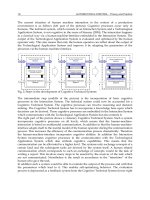
Figure 2.6.12: (a) Boundedness of x
e
at t
0
; (b) uniform boundedness of x
e
; (c) uniform
ultimate boundedness of x
e
; (d) global uniform boundedness of x
e
.
Copyright © 2004 by Marcel Dekker, Inc.
65
EXAMPLE 2.6–5: Stability of the Origin
1. Consider the damped pendulum of Example 2.3.1a. Its equilibrium points
are at [n
π
0]
T

, n=0, ±1,…. The stability of these points can be studied
from the stability of the origin of the system

2. Consider the rigid robot equations of Example 2.3.2, and assume
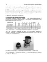
Figure 2.6.13: Example 2.6.4-a: (a)x
1
(0)=x
2
(0)=1 (b) x
1
(0)=x
2
(0)=0.1
2.6 Stability Theory
Copyright © 2004 by Marcel Dekker, Inc.
Introduction to Control Theory66
that a desired trajectory is specified by

Therefore, we can define the new system by choosing z=x
d
-x so that
Figure 2.6.14: Example 2.6.4-b: (a)x
1
(0)=x
2
(0)=1 (b) x
1
(0)=x
2
(0)=1

Copyright © 2004 by Marcel Dekker, Inc.
67
and verify that z
e
=0 is the desired equilibrium point of the modified system if
x
e
=x
d
is the desired equilibrium trajectory of the robot.
᭿
2.7 Lyapunov Stability Theorems
Lyapunov stability theory deals with the behavior of unforced nonlinear
systems described by the differential equations
(2.7.1)
where without loss of generality, the origin is an equilibrium point of (2.7.1).
It may seem to the reader that such a theory is not needed since all we had
to do in the examples of the previous section is to solve the differential
equations, and study the time evolution of a norm of the state vector. There
are at least two reasons why Lyapunov theory is needed. The first is that
Lyapunov theory will allow us to determine the stability of a particular
equilibrium point without actually solving the differential equations. This,
as is well known to any student of nonlinear differential equations, is a
large saving. The second and related reason for using Lyapunov theory is
that it provides us with qualitative results to the stability questions, which
may be used in designing stabilizing controllers of nonlinear dynamical
systems.
We shall first assume that any necessary conditions for (2.7.1) to have a
unique solution are satisfied [Khalil 2001], [Vidyasagar 1992]. The unique
solution corresponding to x(t

0
)=x
0
is x(t, t
0
, x
0
) and will be denoted simply as
x(t). Before we actually introduce Lyapunov’s theorems, we review certain
classes of functions which will simplify the statement of Lyapunov theorems.
Functions of Class K
Consider a continuous function α:ℜ→ℜ
DEFINITION 2.7–1 We say that a belongs to class K, if
1.
α
(0)=0
2.
α
(x)>0, for all x>0
3.
α
is nondecreasing, i.e.
α
(x
1
)Ն
α
(x
2
) for all x

1
>x
2
.
᭿
2.7 Lyapunov Stability Theorems
Copyright © 2004 by Marcel Dekker, Inc.
Introduction to Control Theory68
EXAMPLE 2.7–1: Class K Functions
The function
α
(x)=x
2
is a class K function. The function
α
(x)=x
2
+1 is not a
class K function because (1) fails. On the other hand,
α
(x)=-x
2
is not a class
K function because (2) and (3) fail.
᭿
DEFINITION 2.7–2 In the following, ℜ
+
=[0,
∞).
1. Locally Positive Definite: A continuous function V:ℜ

+
×ℜ
n
→R is locally
positive definite (l.p.d) if there exists a class K function a(.) and a
neighborhood N of the origin of ℜ
n
such that
V(t, x)Ն
α
(||x||)
for all tՆ0, and all x∈N.
2. Positive Definite: The function V is said to be positive definite (p.d) if
N=ℜ
n
.
3. Negative and Local Negative Definite: We say that V is (locally) negative
definite (n.d) if -V is (locally) positive definite.
᭿
EXAMPLE 2.7–2: Locally Positive Definite Functions
[Vidyasagar 1992] The function is l.p.d but not
p.d, since V(t, x)=0 at x=(0, π/2). On the other hand,
is not even l.p.d because V(t, x)→0 as t→∞ for any x. The function
is p.d.
᭿
DEFINITION 2.7–3
In the following,
1. Locally Decrescent: A continuous function is locally
decrescent if There exists a class K function ß(.) and a neighborhood N
of the origin of such that

V(t, x)Յß(||x||)
for all tՆ0 and all x∈
Ν.
Copyright © 2004 by Marcel Dekker, Inc.
69
2. Decrescent: We say that V is decrescent if N=ℜ
n
.
᭿
EXAMPLE 2.7–3: Decrescent Functions
[Vidyasagar 1992] The function
is locally but
not globally decrescent. On the other hand, is globally
decrescent.
᭿
DEFINITION 2.7–4 Given a continuously differentiate function V: ℜ
+
×ℜ
n
→
R together with a system of differential equations (2.7.1), the derivative of V
along (2.7.1) is defined as a function V: ℜ
+
×ℜ
n
→R given by

᭿
EXAMPLE 2.7–4: Lyapunov Functions
Consider the function of Example 2.7.3 and assume

given a system

Then, the derivative of V(t, x) along this system is

᭿
Lyapunov Theorems
We are now ready to state Lyapunov Theorems, which we group in Theorem
2.7.1. For the proof, see [Khalil 2001], [Vidyasagar 1992].
THEOREM 2.7–1: Lyapunov
Given the nonlinear system

2.7 Lyapunov Stability Theorems
Copyright © 2004 by Marcel Dekker, Inc.
Introduction to Control Theory70
with an equilibrium point at the origin, i.e. f(t, 0)=0, and let N be a
neighborhood of the origin of size
⑀
i. e.

Then
1. Stability: The origin is stable in the sense of Lyapunov, if for x∈
Ν
, there
exists a scalar function V(t, x) with continuous partial derivative such
that
(a) V(t, x) is positive definite
(b) V is negative semi-definite
2. Uniform Stability: The origin is uniformly stable if in addition to (a) and
(b) V(t, x) is decrescent for x∈
Ν.

3. Asymptotic Stability: The origin is asymptotically stable if V(t, x) satisfies
(a) and is negative definite for x∈
Ν.
4. Global Asymptotic Stability: The origin is globally, asymptotically stable
if V(t, x) verifies (a), and V(t, x) is negative definite for all x∈ℜ
n

i.e. if
N=ℜ
n
.
5. Uniform Asymptotic Stability: The origin is UAS if V(t, x) satisfies (a),
V(t, x) is decrescent, and V(t,x) is negative definite for x∈
Ν.
6. Global Uniform Asymptotic Stability: The origin is GUAS if N=ℜ
n
,

and
if V(t, x) satisfies (a), V(t,x) is decrescent, V(t,x) is negative definite and
V(t, x) is radially unbounded, i.e. if it goes to infinity uniformly in time
as ||x||→∞.
7. Exponential Stability: The origin is exponentially stable if there exists
positive constants
α
, ß, γ such that

8. Global Exponential Stability: The origin is globally exponential stable if
it is exponentially stable for all x∈ℜ
n

.
᭿
The function V(t, x) in the theorem is called a Lyapunov function. Note that
the theorem provides sufficient conditions for the stability of the origin and
that the inability to provide a Lyapunov function candidate has no indication
on the stability of the origin for a particular system.
Copyright © 2004 by Marcel Dekker, Inc.
71
EXAMPLE 2.7–5: Stability via Lyapunov Functions
1. Consider the system described by

and choose a Lyapunov function candidate

Then the origin may be shown to be a stable equilibrium point.
2. Consider the Mathieu equation described in Example 2.6.3. Let the
Lyapunov function candidate be given by

The origin is then shown to be a US equilibrium point.
3. The system given in Example 2.6.3–5, has a GES equilibrium point at
the origin. This may be shown by considering a Lyapunov function
candidate
V(x)=x
2

which leads to

Then,
0.5x
2
ՅV(x)Յ2x

2

and

The above inequalities hold for any x∈ℜ
n
.
2.7 Lyapunov Stability Theorems
Copyright © 2004 by Marcel Dekker, Inc.
Introduction to Control Theory72
4. Let

and pick a Lyapunov function candidate

so that

so that the origin is SL.
᭿
Lyapunov Theorems may be used to design controllers that will stabilize a
nonlinear system such as a robot. In fact, if one chooses a Lyapunov function
candidate V(t, x), then finding its total derivative V(t, x) will exhibit an
explicit dependence on the control signal. By choosing the control signal to
make V(t, x) negative definite, stability of the closed-loop system is
guaranteed. Unfortunately, it is not always easy to guarantee the global
asymptotic stability of an equilibrium point using Lyapunov Theorem. This
is due to the fact, that V(t, x) may be shown to be negative but not necessarily
negative-definite. If the open-loop system were autonomous, Lyapunov theory
is greatly simplified as shown in the next section.
The Autonomous Case
Suppose the open-loop system is not autonomous, i.e. is not explicitly

dependent on t, then a time-independent Lyapunov function candidate V(x)
may be obtained and the positive definite conditions are greatly simplified as
described next.
LEMMA 2.7–1: A time invariant continuous function V(x) is positive definite
if V(0)=0 and V(x)>0 for x≠0. It is locally positive definite if the above holds
in a neighborhood of the origin ᭿
Note that the condition that V(0)=0 is not necessary and that as long as
V(0) is bounded above the Lyapunov results hold without modification.
Copyright © 2004 by Marcel Dekker, Inc.
73
With the above simplification, the Lyapunov results hold except that no
distinction is made between uniform and regular stability results.
EXAMPLE 2.7–6: Uniform Stability via Lyapunov Functions
Consider again the damped pendulum described by

and obtain a state-space by choosing x
1
=
θ
and then a Lyapunov
function candidate is

so that and the origin is SL and actually USL.
᭿
EXAMPLE 2.7–7: Uniform Stability via Lyapunov Functions
This example illustrates the local asymptotic, uniform stability of the origin
for the system
(1)
Choose then

which is strictly less than zero for all
᭿
Sometimes, and although V(x) is only non-positive, LaSalle’s theorem
[LaSale and Lefschetz 1961], [Khalil 2001] may be used to guarantee the
global asymptotic stability of the equilibrium point as described in the
next theorem.
2.7 Lyapunov Stability Theorems
Copyright © 2004 by Marcel Dekker, Inc.
Introduction to Control Theory74
THEOREM 2.7–2: LaSalle
Given the autonomous nonlinear system

and let the origin be an equilibrium point. Then,
1. Asymptotic Stability: Suppose a Lyapunov function V(x) has been found
such that for , V(x)>0 and Then the origin is
asymptotically stable if and only if only at x=0.
2. Global Asymptotic Stability: The origin is GAS if above and
V(x) is radially unbounded.
᭿
Unfortunately, in many applications with time-varying trajectories, the open-
loop systems are not autonomous, and more advanced results such as the
ones described later will be called upon to show global asymptotic stability.
EXAMPLE 2.7–8: LaSalle Theorem
Consider the autonomous system

The origin is an equilibrium point. Moreover, consider a Lyapunov function
candidate

Leading to

Since for all x
1
=x
2
, we need to check whether the origin is the only
point where It can be seen from the state equation that x
1
=x
2
can
only happen at the origin, therefore the origin is GAS.
᭿
Copyright © 2004 by Marcel Dekker, Inc.
75
Note that LaSalle’s theorem is actually more general than we have
described. In fact, it can be used to ascertain the stability of sets rather than
just an equilibrium point. The basic idea is that since V(x) is lower bounded
V(x)>c, then the derivative V has to gradually vanish, and that the trajectory
is eventually confined to the set where V=0. The following definitions is
useful in explaining the more general LaSalle’s theorem.
DEFINITION 2.7–5 A set G is said to be an invariant set of a dynamical
system if every trajectory which starts in G remains in G. ᭿
As examples of invariant sets, we can give the whole state-space, an
equilibrium point and a limit cycle. By using this concept, LaSalle was able
to describe the convergence to sets rather than to just equilibrium points.
For example, we can use this result to show that the limit cycle is a stable
attracting set of the Van der Pol oscillator.
The Linear Time-Invariant Case
In the case where the system under consideration is linear and time-invariant,
Lyapunov theory is well developed and the choice of a Lyapunov function is

simple. In fact, in this case, the various stability concepts in definitions 2.6.1
are identical. Lyapunov theory then provides necessary as well as sufficient
conditions for stability as discussed in this section. For the proofs consult
[Khalil 2001].
THEOREM 2.7–3: Given a linear time-invariant system

The system is stable if and only if there exists a positive definite solution P to
the equation
A
T
P+PA=-Q
where Q is an arbitrary positive-definite matrix. ᭿
Note that the stability of the whole system was obtained in the last theorem
since in this case, the origin is the unique equilibrium point and its stability is
equivalent to the system being stable. In addition, no reference was made to
what kind of stability is implied since all stability concepts are equivalent in
the very special case of linear, time-invariant systems [Khalil 2001]. Also
note that this result is equivalent to testing that all eigenvalues of A have
negative real parts [Kailath 1980]. In the following, we include a table
summarizing Lyapunov Stability theorems.
2.7 Lyapunov Stability Theorems
Copyright © 2004 by Marcel Dekker, Inc.
Introduction to Control Theory76
Lyapunov Stability Theorems
1. Autonomous Systems: , such that
• The origin is an equilibrium point.
• The set .
• There exists V(x) continuous, continuously differentiate, V(0)=0
2. Non-autonomous Systems: x=f(t, x), such that
• The origin is an equilibrium point at t=t

0
.
• The set .
• There exists V(t, x) continuous, continuously differentiate in t and
x, V(t, 0)=0
•
α
(||x||), ß(||x||), and γ(||x||) class K functions.
Lyapunov Theorems may be used to design controllers that can stabilize
linear time-invariant systems as described in the next example.
Copyright © 2004 by Marcel Dekker, Inc.
77
EXAMPLE 2.7–9: Stability of PD Controllers for Rigid Robots
Consider the rigid robot example and the torque input of Example 2.3.2.
The resulting linear system is given by

The equilibrium point is x
e
=[0
T
0
T
]
T
. It is then easy to find K
p
and K
v
to
stabilize the equilibrium point. In fact, let Q=I and consider the Lyapunov

equation of theorem 2.7.3
A
T
P+PA=-I
which reduces to

where

The solution of these equations will provide a stabilizing controller for the
robot. In particular, the choices of K
p
and K
v
of Example 2.6.3(part 5) will
make the origin a GES equilibrium.
᭿
Convergence Rate
Although Lyapunov stability theory does not directly give an indication of
the transient behavior of the system, it may actually be used to estimate the
convergence rate for linear systems. In order to see this, consider the following
inequalities which are a result of Rayleigh-Ritz theorem 2.5.2,
x
T
λ
min
(P)xՅx
T
PxՅx
T
λ

max
(P)x (2.7.2)
2.7 Lyapunov Stability Theorems
Copyright © 2004 by Marcel Dekker, Inc.
Introduction to Control Theory78
then, note
(2.7.3)
Now, we can show by separation of variables and integrating that
x
T
␭
min
(P)xՅV(t)ՅV(0)e
-␥t
(2.7.4)
or that
(2.7.5)
Therefore, x(t) is approaching the origin at rate faster than ␥/2. In fact, it
can be shown that the fastest convergence rate estimate is obtained when
Q=I.
Krasovskii Theorem
There are some cases when a Lyapunov function for autonomous nonlinear
systems is easily obtained using Krasovkii’s theorem stated below.
THEOREM 2.7–4: Consider the autonomous nonlinear system x=f(x) with
the origin being an equilibrium point. Let A(x)=∂f/∂x. Then, a sufficient
condition for the origin to be AS is that there exists 2 symmetric positive-
definite matrices, P and Q such that for all x≠0, the matrix
F(x)=A(x)
T
P+PA(x)+Q (1)

is Ն0 in some ball B about the origin. The function V(x)=f(x)
T
Pf(x) is then a
Lyapunov function for the system. If B= and if V(x) is radially unbounded
then the system is GAS.
Copyright © 2004 by Marcel Dekker, Inc.
79
EXAMPLE 2.7–10: Krasovkii’s Theorem
Consider the nonlinear system described by

where f(0)=g(0)=0. Let us find the Jacobian matrix

Let P=I, Q=
⑀
I and check the conditions on the system which would look
like

which should be Ն0.
᭿
On the other hand, suppose we have the linear time-invariant system

The transfer function is then given by
P(s)=C(sI-A)
-1
B
Note that P(s) is strictly-proper. The following stability result then holds
[Desoer and Vidyasagar 1975].
THEOREM 2.7–5: Suppose P(s) is a stable transfer function then
1. If u(t)∈L
∞

i.e. u(t) is bounded, then so is y(t) and .
2. If lim
t→∞
u(t)=0 then lim
t→∞
y(t)=0.
2.7 Lyapunov Stability Theorems
Copyright © 2004 by Marcel Dekker, Inc.
Introduction to Control Theory80
3. If u(t)∈L
2
, then .
᭿
EXAMPLE 2.7–11: Input/Output Stability of Rigid Robots
Consider the closed-loop robot of Example 2.7.9. Its input/output behavior
is described by a set of n decoupled differential equations

If . Then the transfer function between each
U
i
(s) and Q
i
(s) is

Note that all P
i
(s) are stable if k
vi
and k
pi

are both positive. Assume for the
purposes of illustration that k
vi
=3 and k
pi
=2, and that u
i
=sin (t). Note that u
i
is bounded and let us find the output y
i
(t).
y
i
(t)=-0.2e
-2t
+0.5e
-t
-0.32 cos(t+0.32)
which is bounded above by 0.62 and below by -0.02. The derivative of y(t)
is also bounded. On the other hand, suppose the input is u
i
(t)=e
-3t
then the
output is
y
i
(t)=0.5e
-t

-e-
2t
+0.5e
-3t

Since lim
t→∞
u
i
(t)=0, then so is lim
t→∞
y
i
(t)=0.
᭿
2.8 Input/Output Stability
When dealing with nonlinear systems, stability in the sense of Lyapunov
does not necessarily imply that a bounded input will result in a bounded
output. This fact is shown in the next example.
Copyright © 2004 by Marcel Dekker, Inc.
81
EXAMPLE 2.8–1: Input/Output Versus Lyapunov Stability
Consider the time-varying system

The system is asymptotically stable with a single equilibrium point at y
e
=0.
On the other hand, a unit step input (which is definitely bounded) starting at
t=0 will lead to the response

which grows unbounded as t increases.
᭿
Therefore, we need to discuss the conditions under which a bounded input
will result in a bounded output [Boyd and Barratt], [Desoer and Vidyasagar
1975]. This was actually presented when discussing the system-induced
norms (see Definition 2.5.7) and the current discussion should serve to
contrast these concepts with Lyapunov stability. Consider the nonlinear
system
(2.8.1)
y(t)=g[x(t), t, u(t)] (2.8.2)
DEFINITION 2.8–1 The dynamical system (2.8.1) is bounded-input-
bounded-output (BIBO) stable if for any
||u(t)||ՅM<8
there exist finite γ>0 and b such that
||y(t)||ՅγM+b
᭿
Note that BIBO stability implies the uniform boundedness of all equilibrium
states.
2.8 Input/Output Stability
Copyright © 2004 by Marcel Dekker, Inc.
Introduction to Control Theory82
EXAMPLE 2.8–2: BIBO Stability
Consider the system
y(t)=u
2
(t)
It is BIBO stable since for any input u(t) such that |u(t)|<M<∞, the output is
bounded by M
2
.

᭿
2.9 Advanced Stability Results
In this section we review some advanced stability concepts. These results
will be used in showing the closed-loop stability of systems when robust or
adaptive controllers are used. If the reader is only interested in implementing
these controllers, this section may be skipped. On the other hand, anyone
interested in designing new controllers should be aware of the results presented
here.
Passive Systems
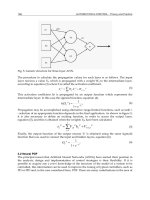
Given a nonlinear system shown in Figure 2.9.1, we are interested in studying
the stability of such a system based on input-output measurements only.
Motivated by energy concepts in network theory, such as
[Stored Energy]=[External Power Input]+[Internal power Generation]
One can study the internal stability of all kinds of systems. In general,
the external power input is the scalar product y
T
u of an input effort or
flow u and an output flow or effort y. The last equation then takes on the
form
(2.9.1)
In many cases (e.g. isolated system) g(t)=0 and one can use the stored
Energy
(2.9.2)
Copyright © 2004 by Marcel Dekker, Inc.
Introduction to Control Theory84
Suppose the robot is representing a system whose input is
␶
and whose
output is the joint velocity q. Let the sum of the kinetic energy and potential
energy of the robot be denote by the Hamiltonian H and recall [Ortega and

Spong 1988]

then

which proves that from
␶
to q, the rigid robot is a passive system.
᭿
A passive system is in effect one that does not create energy.
Positive-Real Systems
If the system under consideration is linear and time-invariant, then passivity
is equivalent to positivity and may be tested in the frequency domain
[Narendra and Taylor 1973]. In fact, let us describe positive-real systems
and discuss some of their properties. Consider the multi-input-multi-output
linear time-invariant system

where x is an n vector, u is an m vector, y is a p vector, A, B, C, and D are of
the appropriate dimensions. The corresponding transfer function matrix is
P(s)=C(sI-A)
-1
B+D
We will assume that the system has an equal number of inputs and outputs,
i.e. p=m. To simplify our notation we will denote the Hermitian part of a
real, rational transfer matrix T(s) by where s*
is the complex conjugate of s. A number of definitions have been given for
SPR functions and matrices [Narendra and Taylor 1973]. It appears that the
most useful definition for control applications is the following.
DEFINITION 2.9–2 An m×m matrix T(s) of proper real rational functions
which is not identically zero is positive-real or PR if
Copyright © 2004 by Marcel Dekker, Inc.

85
1. All elements of T(s) have no poles in the region Re(s)>0,
2. Any poles of T(s) on the jw axis are simple with positive-definite residues,
and
3. The matrix He[T(s)] is positive semidefinite for Re(s)>0.
᭿
EXAMPLE 2.9–2: PR Matrices
Consider the matrix

This matrix is PR as can be checked.
DEFINITION 2.9–3 An m×m matrix T(s) of proper real rational functions
which is not identically zero is strictly-positive-real or SPR if
1. All elements of T(s) have no poles in the region Re(s)Ն0, and
2. The matrix He[T(s)] is positive definite for Re(s)>0.
᭿
EXAMPLE 2.9–3: SPR Matrices
Consider the matrix

This matrix is SPR as can be checked.
᭿
Lure’s Problem
Consider the following feedback interconnected system
(2.9.3)
2.9 Advanced Stability Results
Copyright © 2004 by Marcel Dekker, Inc.
Introduction to Control Theory86
where
φ
is continuous in both arguments. Lure then stated the following
Absolute Stability problem which became known as Lure’s Problem: Suppose

the system described by the above equations is given where:
1. All eigenvalues of A have negative real parts or that A has one eigen-
value at the origin while the rest of them is in the open left-half plane
(OLHP), and
2. (A, b) is controllable, and
3. (c, A) is observable, and
4. The nonlinearity
φ
(.,.)

satisfies
(a)
φ(
t,0)=0;᭙tՆ0 and
(b)
Then, find conditions on the linear system (A, B, C, D) such that x=0 is a
GAS equilibrium point of the closed-loop system.
Note that sometimes when we know more about the nonlinearity
φ,
the
last condition above is replaced by the following:

where k
2
Նk
1
Ն0 are constants. We then say that
φ
belongs to the sector
[k

1
, k
2
].
The first attempt to solve this problem was made by Aizerman in what is
now known as Aizerman’s conjecture [Vidyasagar 1992] followed by the
efforts of Kalman [Vidyasagar 1992]. The correct solution however, was not
available until the
In order to present the correct results, we need to present the KY and
MKY lemmas.
The MKY Lemma
The following lemmas are versions of the Meyer-Kalman-Yakubovich
(MKY) lemma which appears in [Narendra and Taylor 1973], [Khalil 2001]
amongst other places, and will be useful in designing adaptive controllers
for robots.
LEMMA 2.9–1: Meyer-Kalman-Yakubovitch Let the system (2.9.3) with
D=0 be controllable. Then the transfer function c(sI-A)
-1
b is SPR if and
only if
Copyright © 2004 by Marcel Dekker, Inc.
87
1. For any symmetric, positive-definite Q, there exists a symmetric, positive-
definite P solution of the Lyapunov equation
A
T
P+PA=-Q
2. The matrices B and C satisfy
C=B
T

P
᭿
The MKY Lemma gives conditions under which a transfer matrix has a
degree of robustness. Note that the conditions depend on both the input and
output matrices and thus a particular system may be SPR for a certain choice
of input/output pairs and not SPR for others. A modified version of the KY
lemma which relaxes the condition of controllability is given next.
LEMMA 2.9–2: Meyer-Kalman-Yakubovitch Given vector b, an
asymptotically stable A, a real vector v, scalars γՆ0 and
⑀
>0, and a positive-
definite matrix Q, then, there exist a vector q and a symmetric positive definite
P such that
1.
2.

if and only if
1. is small enough and,
2. the transfer function γ/2+v
T
(sI-A)
-1
b is SPR
᭿
In most of our applications, q=0. These lemmas find many applications in
nonlinear systems. It is usually possible to divide a nonlinear system into a
linear feed-forward subsystem, and a nonlinear, passive feedback. The
challenge is then to make the linear subsystem SPR so that the stability of the
combined system is guaranteed.
2.9 Advanced Stability Results

Copyright © 2004 by Marcel Dekker, Inc.
Introduction to Control Theory88
2.10 Useful Theorems and Lemmas
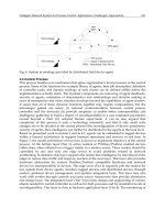
Consider the block diagram shown in Figure 2.9.2. The blocks labelled H
1
and H
2
represent two systems (linear or nonlinear) which operate on the
inputs e
1
and e
2
as follows
y
1
=H
1
e
1
=H
1
(u
1
-y
2
)
y
2
=H
2

e
2
-H
2
(u
2
+y
1
)
Let H
1
be an m×p matrix function, and H
2
be a p×m matrix function.
Therefore, u
1
and y
2
are p×11 vectors, while u
2
and y
1
are m×11 vectors. The
first theorem gives sufficient conditions to guarantee that the closed-loop
system shown in Figure 2.9.2 is BIBO stable and is given in [Desoer and
Vidyasagar 1975].
Small-Gain Theorem
THEOREM 2.10–1: Small gain Theorem Let H
1
: and H

2
:
. Therefore H
1
and H
2
satisfy the inequalities

for all T
⑀
[0,∞) and suppose that . If

Figure 2.9.2: Feedback interconnection of two nonlinear systems.
Copyright © 2004 by Marcel Dekker, Inc.