Robot Manipulator Control Theory and Practice - Frank L.Lewis Part 6 doc

Computed-Torque Control186
(4.4.3)
To demonstrate the influence of the input ␶(t)on the tracking error, differe-
ntiate twice to obtain

Solving now for in (4.4.2) and substituting into the last equation yields
(4.4.4)
Defining the control input function
(4.4.5)
and the disturbance function
(4.4.6)
we may define a state by
(4.4.7)
and write the tracking error dynamics as
(4.4.8)
This is a linear error system in Brunovsky canonical form consisting of n
pairs of double integrators 1/s
2
, one per joint. It is driven by the control input
u(t) and the disturbance w(t). Note that this derivation is a special case of the
general feedback linearization procedure in Section 3.4.
The feedback linearizing transformation (4.4.5) may be inverted to yield
(4.4.9)
We call this the computed-torque control law. The importance of these
manipulations is as follows. There has been no state-space transformation in
going from (4.4.1) to (4.4.8). Therefore, if we select a control u(t) that stabilizes
(4.4.8) so that e(t) goes to zero, then the nonlinear control input given by
␶(t)(4.4.9) will cause trajectory following in the robot arm (4.4.1). In fact,
substituting (4.4.9) into (4.4.2) yields
Copyright © 2004 by Marcel Dekker, Inc.

187

or
(4.4.10)
which is exactly (4.4.8).
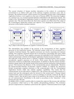
Figure 4.4.1: Computed-torque control scheme, showing inner and outer loops.
The stabilization of (4.4.8) is not difficult. In fact, the nonlinear
transformation (4.4.5) has converted a complicated nonlinear controls design
problem into a simple design problem for a linear system consisting of n
decoupled subsystems, each obeying Newton’s laws.
The resulting control scheme appears in Figure 4.4.1. It is important to
note that it consists of an inner nonlinear loop plus an outer control signal
u(t). We shall see several ways for selecting u(t). Since u(t) will depend on q(t)
and q
.
(t), the outer loop will be a feedback loop. In general, we may select a
dynamic compensator H(s) so that
U(s)=H(s)E(s). (4.4.11)
H(s) can be selected for good closed-loop behavior. According to (4.4.10), the
closed-loop error system then has transfer function
T(s)=s
2
I-H(s). (4.4.12)
4.4 Computed-Torque Control
Copyright © 2004 by Marcel Dekker, Inc.
Computed-Torque Control188
It is important to realize that computed-torque depends on the inversion of
the robot dynamics, and indeed is sometimes called inverse dynamics control
In fact, (4.4.9) shows that ␶(t) is computed by substituting
d

–u for in (4.4.2);
that is, by solving the robot inverse dynamics problem. The caveats associated
with system inversion, including the problems resulting when the system has
non-minimum-phase zeros, all apply here. (Note that in the linear case, the
system zeros are the poles of the inverse. Such nonminimum-phase notions
generalize to nonlinear systems.) Fortunately for us, the rigid arm dynamics
are minimum phase.
There are several ways to compute (4.4.9) for implementation purposes.
Formal matrix multiplication at each sample time should be avoided. In some
cases the expression may be worked out analytically. A good way to compute
the torque ␶(t) is to use the efficient Newton-Euler inverse dynamics formulation
[Craig 1985] with
d
–u in place of (t).
The outer-loop signal u(t) can be chosen using many approaches, including
robust and adaptive control techniques. In the remainder of this chapter we
explore some choices for u(t) and some variations on computed-torque control.
PD Outer-Loop Design
One way to select the auxiliary control signal u(t) is as the proportional-plus-
derivative (PD) feedback,
(4.4.13)
Then the overall robot arm input becomes
(4.4.14)
This controller is shown in Figure 4.4.6 with K
i
=0. The closed-loop error
dynamics are
(4.4.15)
or in state-space form,
(4.4.16)

The closed-loop characteristic polynomial is
(4.4.17)
Choice of PD Gains. It is usual to take the n×n gain matrices diagonal so
that
Copyright © 2004 by Marcel Dekker, Inc.
189
(4.4.18)
Then
(4.4.19)
and the error system is asymptotically stable as long as the K
vi
and K
pi
are
all positive. Therefore, as long as the disturbance w(t) is bounded, so is the
error e(t). In connection with this, examine (4.4.6) and recall from Table
3.3.1 that M
-1
is upper bounded. Thus boundedness of w(t) is equivalent to
boundedness of ␶
d
(t).
It is important to note that although selecting the PD gain matrices diagonal
results in decoupled control at the outer-loop level, it does not result in a
decoupled joint-control strategy. This is because multiplication by M(q) and
addition of the nonlinear feedforward terms N (q, q
.
) in the inner loop scrambles
the signal u(t) among all the joints. Thus, information on all joint positions
q(t) and velocities q

.
(t) is generally needed to compute the control ␶(t) for any
one given joint.
The standard form for the second-order characteristic polynomial is
(4.4.20)
with ␨ the damping ratio and
␻
n
the natural frequency. Therefore, desired
performance in each component of the error e(t) may be achieved by selecting
the PD gains as
(4.4.21)
with ␨,
␻
n
the desired damping ratio and natural frequency for joint error i. It
may be useful to select the desired responses at the end of the arm faster than
near the base, where the masses that must be moved are heavier.
It is undesirable for the robot to exhibit overshoot, since this could cause
impact if, for instance, a desired trajectory terminates at the surface of a
workpiece. Therefore, the PD gains are usually selected for critical damping
␨=1. In this case
(4.4.22)
Selection of the Natural Frequency. The natural frequency
␻
n
governs the
speed of response in each error component. It should be large for fast responses
and is selected depending on the performance objectives. Thus the desired
trajectories should be taken into account in selecting

␻
n
. We discuss now
some additional factors in this choice.
4.4 Computed-Torque Control
Copyright © 2004 by Marcel Dekker, Inc.
Computed-Torque Control190
There are some upper limits on the choice for
␻
n
[Paul 1981]. Although the
links of most industrial robots are massive, they may have some flexibility.
Suppose that the frequency of the first flexible or resonant mode of link i is
(4.4.23)
with J the link inertia and k
r
the link stiffness. Then, to avoid exciting the
resonant mode, we should select
␻
n
<
␻
r
/2. Of course, the link inertia J changes
with the arm configuration, so that its maximum value might be used in
computing
␻
r
.
Another upper bound on

␻
n
is provided by considerations on actuator
saturation. If the PD gains are too large, the torque τ(t) may reach its upper
limits.
Some more feeling for the choice of the PD gains is provided from error-
boundedness considerations as follows. The transfer function of the closed-
loop error system in (4.4.15) is
(4.4.24)
or if K
v
and K
p
are diagonal,
(4.4.25)
(4.4.26)
We assume that the disturbance and M
-1
are bounded (Table 3.3.1), so that
(4.4.27)
with m
—

and d
—
known for a given robot arm. Therefore,
(4.4.28)
(4.4.29)
Now selecting the L
2

—norm, the operator gain ||H(s)||
2
is the maximum
value of the Bode magnitude plot of H(s). For a critically damped system,
(4.4.30)
Therefore,
Copyright © 2004 by Marcel Dekker, Inc.
191
(4.4.31)
Moreover (see the Problems),
(4.4.32)
so that
(4.4.33)
Thus, in the case of critical damping, the position error decreases with k
pi
and
the velocity error decreases with k
vi
.
EXAMPLE 4.4–1: Simulation of PD Computed-Torque Control
In this example we intend to show the detailed mechanics of simulating a
PD computed-torque controller on a digital computer.
a. Computed-Torque Control Law
In Example 3.2.2 we found the dynamics of the two-link planar elbow arm
shown in Figure 4.2.1 to be
(1)
These are in the standard form
(2)
Take the link masses as 1 kg and their lengths as 1 m.
The PD computed-torque control law is given as

4.4 Computed-Torque Control
Copyright © 2004 by Marcel Dekker, Inc.
Computed-Torque Control192
(3)
with the tracking error defined as
e=q
d
-q. (4)
b. Desired Trajectory
Let the desired trajectory q
d
(t) have the components
θ
1d
=g
1
sin (2πt/T)
θ
2d
=g
2
cos (2πt/T) (5)
with period T=2 s and amplitudes g
i
=0.1 rad≈6 deg. For good tracking select
the time constant of the closed-loop system as 0.1 s. For critical damping, this
means that K
v
=diag{k
v

}, K
P
=diag{k
p
}, where
(6)
It is important to realize that the selection of controller parameters such as the
PD gains depends on the performance objectives-in this case, the period of the
desired trajectory.
c. Computer Simulation
Let us simulate the computed-torque controller using program TRESP in
Appendix B. Simulation using commercial packages such as MATLAB and
SIMNON is quite similar.
The subroutines needed for TRESP are shown in Figure 4.4.2. They are
worth examining closely. Subroutine SYSINP (ITx, t) is called once per Runge-
Kutta integration period and generates the reference trajectory q
d
(t), as well
as q
d
(t), and q
d
(t). Note that the reference signal should be held constant
during each integration period.
Copyright © 2004 by Marcel Dekker, Inc.
Computed-Torque Control194
Copyright © 2004 by Marcel Dekker, Inc.
195
Subroutine F(time, x, xp) is called by Runge-Kutta and contains the
continuous dynamics. This includes both the controller and the arm dynamics.

The state to be integrated is and the subroutine should
compute the state derivative x (i.e., xp, which signifies x—prime).
Subroutine CTL(x) contains the controller (3). Note the structure of this
subroutine. First, the tracking error e(t) and its derivative are computed. Then
M(q) and are computed. Finally, (3) is
manufactured.
Figure 4.4.2: Subroutines for simulation using TRESP.
Figure 4.4.3: Joint angles θ
1
(t) and θ
2
(t) (red).
4.4 Computed-Torque Control
Copyright © 2004 by Marcel Dekker, Inc.
Computed-Torque Control196
Subroutine ARM(x, xp) contains the robot dynamics. First, M(q) and M
-
1
(q) are computed, and then N(q,q). The state derivatives are then determined.
The results of the simulation are shown in the figures. Figure 4.4.3 shows
the joint angles. Figure 4.4.4 shows the joint errors. The initial conditions
result in a large initial error that vanishes within 0.6 s. Figure 4.4.5 shows the
control torques; the larger torque corresponds to the inner motor, which must
move two links.
It is interesting to note the ripples in e(t) that appear in Figure 4.4.4. These
are artifacts of the integrator. The Runge-Kutta integration period was T
R
=0.01
s. When the simulation was repeated using T
R

=0.001 s, the tracking error was
exactly zero after 0.6 s. It should be zero, since computed-torque, or inverse
dynamics control, is a scheme for canceling the nonlinearities in the dynamics
to yield a second-order linear error system. If all the arm parameters are
exactly known, this cancellation is exact. It is a good exercise to repeat this
simulation using various values for the PD gains (see the Problems).
Figure 4.4.4: Tracking error e
1
(t), e
2
(t) (red).
Copyright © 2004 by Marcel Dekker, Inc.
199
Selecting diagonal control’ gains
(4.4.40)
gives
(4.4.41)
By using the Routh test it can be found that for closed-loop stability we require
that
(4.4.42)
that is, the integral gain should not be too large.
Actuator Saturation and Integrator Windup. It is important to be aware of an
effect in implementing PID control on any actual robot manipulator that can
cause serious problems if not accounted for. Any real robot arm will have
limits on the voltages and torques of its actuators. These limits may or may
not cause a problem with PD control, but are virtually guaranteed to cause
problems with integral control due to a phenomenon known as integrator
windup [Lewis 1992].
Consider the simple case where
␶

=k
i
ε
with
ε
(t) the integrator output. The
torque input
␶
(t)

is limited by its maximum and minimum values
␶
max

and
␶
min
.
If k
i
ε
(t) hits
␶
max
,

there may or not may not be a problem. The problem arises
if the integrator input remains positive, for then the integrator continues to
integrate upwards and k
i

ε
(t) may increase well beyond
␶
max
.

Then, when the
integrator input becomes negative, it may take considerable time for k
i
ε
(t) to
decrease below
␶
max
.

In the meantime
␶
is held at
␶
max
,

giving an incorrect
control input to the plant.
Integrator windup is easy to correct using antiwindup protection in a digital
controller. This is discussed in Section 4.5. The effects of uncorrected windup
are demonstrated in Example 4.4.4.
The next example shows the usefulness of an integral term when there are
unknown disturbances present.

EXAMPLE 4.4–2: Simulation of PID Computed-Torque Control
In Example 4.4.1 we simulated the PD computed-torque controller for a
two-link planar arm. In this example we add a constant unknown
4.4 Computed-Torque Control
Copyright © 2004 by Marcel Dekker, Inc.
Computed-Torque Control200
Figure 4.4.7: Computed-torque controller tracking errors e
1
(t), e
2
(t) (red): (a) PD
control; (b) PID control.
Copyright © 2004 by Marcel Dekker, Inc.
201
Figure 4.4.8: Computed-torque controller torque inputs (N-m): (a) PD control; (b)
PID control.
4.4 Computed-Torque Control
Copyright © 2004 by Marcel Dekker, Inc.
Computed-Torque Control202
disturbance to the arm dynamics and compare PD to PID computed
torque.
Thus let the arm dynamics be
(1)
with
␶
d
a constant disturbance with 1 N-m in each component. This could
model unknown dynamics such as friction, and so on. The value of 1 N-m
represents quite a large bias.
Adding 1 to the computation of the nonlinear terms N1 and N2 in

subroutine arm(x, xp) in Figure 4.4.2 and using the PD computed-torque
controller with k
p
=100, k
v
=20 yields the error plot in Figure 4.4.7(a).
There is a unacceptable residual bias in the tracking error due to the
unmodeled constant disturbance, which is not accounted for in the
computed-torque law. The largest error is 0.033 rad, somewhat less
than 2 deg.
Adding now an integral-error weighting term with k
i
=500 yields the
results in Figure 4.4.7(b), which show a zero steady-state error and are
quite good.
The associated control torques are shown in Figure 4.4.8, which shows
that the torque magnitudes are not appreciably increased by using the
integral term.
To simulate the PID control law, it is necessary to add two additional
states to x in subroutine arm(x, xp). It is convenient to call them x(5) and
x(6), so that the lines added to the subroutine are
xp(5)=e(1).
xp(6)=e(2). (2)
Thus it is now necessary to compute e(1) and e(2) in subroutine arm(x, xp)
for integration purposes.
᭿
Class of Computed-Torque-Like Controllers
An entire class of computed-torque-like controllers can be obtained by
modifying the computed-torque control law to read
(4.4.43)

Copyright © 2004 by Marcel Dekker, Inc.
203
The carets denote design choices for the weighting and offset matrices. One
choice is =M(q), =N(q,q). The calculated control input into the robot arm
is
␶
c
(t).
In some cases M(q) is not known exactly (e.g., unknown payload mass), or
N(q, ) is not known exactly (e.g., unknown friction terms). Then and
could be the best estimate we have for these terms. On the other hand, we
might simply wish to avoid computing M(q) and N(q,q) at each sample time,
or the sample period might be too short to allow this with the available
hardware. From such considerations, we call (4.4.43) an “approximate
computed-torque” controller.
In Table 4.4.1 are given some useful computed-torque-like controllers. As it
turns out, computed torque is quite a good scheme since it has some important
robustness properties. In fact, even if ≠M and ≠N the performance of
controllers based on (4.4.43) can be quite good if the outer-loop gains are selected
large enough. We study robustness formally in Chapter 4.
In the remainder of this chapter we consider various special choices of
and that give some special sorts of controllers. We shall present some
theorems and simulation examples that illustrate the robustness properties of
computed-torque control.
Error Dynamics with Approximate Control Law. Let us now derive the error
dynamics if the approximate computed-torque controller (4.4.43) is applied to
the robot arm (4.4.2). Substituting
␶
c
(t) into the arm equation for

␶
(t) yields

Adding Mq
d
-Mq
d
to the left-hand side and Mu-Mu to the right gives

or
ë=u-∆u+d, (4.4.44)
where the inertia and nonlinear-term model mismatch terms are
(4.4.45)
(4.4.46)
4.4 Computed-Torque Control
Copyright © 2004 by Marcel Dekker, Inc.
205
and the disturbance is
(4.4.47)
This reduces to the error system (4.4.10) if exact computed-torque control
is used so that ∆=0,
δ
=0. Otherwise, the error system is driven by the
desired acceleration and the nonlinear term mismatch
δ
(t). Thus the tracking
error will never go exactly to zero. Moreover, the auxiliary control u(t) is
multiplied by (I -∆), which can make for a very difficult control problem.
Using outer-loop PD feedback so that u(t)=-K
v

e-K
p
e yields the error system
(4.4.48)
The behavior of such systems is not obvious, even if K
v
and K
p
are selected for
good stability of the left-hand side. There are two sorts of problems: first, the
disturbance term d(t), and second the function ∆(K
v
e+K
p
e) of the error and its
derivative.
PD-Plus-Gravity Controller
A useful controller in the computed-torque family is the PD-plus-gravity
controller that results when M=I, N=G(q)-q
d
, with G(q) the gravity term of
the manipulator dynamics. Then, selecting PD feedback for u(t) yields
(4.4.49)
This control law was treated in [Arimoto and Miyazaki 1984], [Schilling
1990]. It is much simpler to implement than the exact computedtorque
controller.
When the arm is at rest, the only nonzero terms in the dynamics (4.4.1)
are the gravity G(q), the disturbance
␶
d

, and possibly the control torque
␶
.
The PD-gravity controller
␶
c
, includes G(q), so that we should expect good
performance for set-point tracking, that is, when a constant q
d
is given so
that q
d
=0. The next result formalizes this. It relies on a Lyapunov proof
(Chapter 1) of the sort that will be of consistent usefulness throughout the
book, drawing especially on the skew-symmetry property in Table 3.3.1.
Thus it is very important to understand the steps in this proof.
4.4 Computed-Torque Control
Copyright © 2004 by Marcel Dekker, Inc.
Computed-Torque Control206
THEOREM 4.4–1: Suppose that PD-gravity control is used in the arm
dynamics (4.4.1) and
␶
d
=0, q
d
=0. Then the steady-state tracking error. e=q
d
-
q is zero.
Proof:

1. Closed-Loop System
Ignoring friction, the robot dynamics are given by
(1)
When q
d
=0, the proposed control law (4.4.49) yields the closed-loop dynamics
(2)
2. Lyapunov Function
Select now the Lyapunov function
(3)
and differentiate to obtain
(4)
Substituting the closed-loop dynamics (2) yields
(5)
Now, the skew symmetry of the first term gives
(6)
The state is , so that V is positive definite but only negative
semidefinite. Therefore, we have demonstrated stability in the sense of
Lyapunov, that is, that the error and joint velocity are both bounded.
3. Asymptotic Stability by LaSalle’s Extension
The asymptotic stability of the system may be demonstrated using Barbalat’s
lemma and a variant of LaSalle’s extension [Slotine and Li 1991] (Chapter
2). Thus it is necessary to demonstrate that the only invariant set contained in
the set V=0 is the origin.
Since V is lower bounded by zero and nonpositive, it follows that V
approaches a finite limit, which can be written
Copyright © 2004 by Marcel Dekker, Inc.
207
(7)
We now invoke Barbalat’s lemma to show that V goes to zero. For this, it is

necessary to demonstrate the uniform continuity of V. We see that
(8)
The demonstrated stability shows that a and q are bounded, whence (2) and
the boundedness of M
-1
(q) (see Table 3.3.1) reveal that q is bounded. Therefore,
V is bounded, whence V is uniformly continuous. This guarantees by Barbalat’s
lemma that V goes to zero.
It is now clear that
goes to zero. It remains to show that the tracking
error e(t) vanishes. Note that when q=0, (2) reveals that
(9)
Therefore, a nonzero e(t) results in nonzero and hence in q≠0, a contradiction.
Therefore, the only invariant set contained in {x(t)|V=0} is x(t)=0. This finally
demonstrates that both e(t) and vanish and concludes the proof. ᭿
Some notes on this proof are warranted. First, note that the Lyapunov
function chosen is a natural one, as it contains the kinetic energy and the
“artificial potential energy” associated with the virtual spring in the control
law [Slotine and Li 1991]. K
p
appears in V while K
v
appears in V.
The proof of Lyapunov stability is quick and easy. The effort comes about
in showing asymptotic stability. For this, it is required to return to the system
dynamics and study it more carefully, discussing issues such as boundedness
of signals, invariant sets, and so on. The fundamental property of skew
symmetry is used in computing V. The boundedness of M
-1
(q) is needed in

Barbalat’s lemma.
The next example illustrates the performance of the PD-gravity controller
for trajectory tracking. In general, if q
d
≠
0, then the PD-gravity controller
guarantees bounded tracking errors. The error bound decreases, that is, the
tracking performance improves, as the PD gains become larger. This will be
EXAMPLE 4.4–3: Simulation of PD-Gravity Controller
In Example 4.4.1 we simulated the exact computed-torque control law on
a two link planar manipulator. Here, let us simulate the PD-gravity
controller. We shall take the same arm parameters and desired trajectory.
4.4 Computed-Torque Control
Copyright © 2004 by Marcel Dekker, Inc.
made rigorous in Chapter 4.
Computed-Torque Control208
Assuming identical PD gains for each link, the PD-gravity control law for
the two-link arm is
(1)
This is easily simulated by commenting out several lines of code and making
a few other modifications in subroutine CTL(x) of Figure 4.4.2.
For critical damping, the PD gains are selected as
(2)
The results of the PD-gravity controller simulation for several values of w
n
are shown in Figure 4.4.9. As ω
n
, and hence the PD gains, increases, the
tracking performance improves. However, no matter how large the PD gains,
the tracking error never goes exactly to zero, but is bounded about zero by a

ball whose radius decreases as the gains become larger. The performance for
ω
n
=50, corresponding to k
p
=2500, k
v
=100, would be quite suitable for many
applications.
It quite important to note that the dc value of the errors is equal to zero.
One can consider the gravity terms as the “dc portion” of the computed-
torque control law. If they are included in computing the torques, there will
be no error offset.
The associated control input torques are shown in Figure 4.4.10. It is
extremely interesting to note that the torques are smaller for the higher
gains. This is contrary to popular belief, which assumes that the control
torques always increase with increasing PD gains. It is due to the fact that
larger gains give “tighter” performance, and hence smaller tracking errors.
In view of the fact that the errors in Figure 4.4.9(a) have different magnitudes,
it would probably be more reasonable to take the PD gains larger for the
inner link than the outer link.
᭿
Classical Joint Control
A simple controller that often gives good results in practice is obtained by
selecting in (4.4.43)
(4.4.50)
Copyright © 2004 by Marcel Dekker, Inc.
Computed-Torque Control210
Then there results
(4.4.51)

By selecting u
i
to depend only on joint variable i, this describes n decoupled
individual joint controllers and is called independent joint control.
Implementation on an actual robot arm is easy since the control input for
joint i only depends on locally measured variables, not on the variables of the
other joints. Moreover, the computations are easy and do not involve solving
the complicated nonlinear robot inverse dynamics.
During the early days of robotics, independent joint control was popular
[Paul 1981] since it allows a decoupled analysis of the closed-loop system
using single-input/single-output (SISO) classical techniques. It is also called
classical joint control. There are strong arguments even today by several
researchers that this control scheme is always suitable in practical
implementations, and that modern nonlinear control schemes are too
complicated for industrial robotic applications.
A traditional analysis of independent joint control control now follows. It
provides a connection with classical control notions and is important for the
Figure 4.4.9: (Cont.) (c)w
n
=50 rad/s.
Copyright © 2004 by Marcel Dekker, Inc.
Computed-Torque Control212
robot controls designer to understand. See [Franklin et al. 1986] for a reference
on classical control theory.
A simplified dynamical model of a robot arm with electric actuators may
be written as (Section 3.6)
(4.4.52)
with J
m
the actuator motor inertia, B

m
the rotor damping constant, k
m
the
torque constant, k
b
the back emf constant, R the armature resistance, and r
i
the gear ratio for joint i. The motor angle is denoted
θ
i
(t). The constant portions
of the diagonal elements of M(q) are denoted m
ii
. The time-varying portions
of these elements, as well as the off-diagonal elements of M(q), the nonlinear
terms N(q, ), and any disturbances
␶
d
are all lumped into the disturbance
d
i
(t). Thus d
i
(t) contains the effects on joint i of all the other joints. The control
input is the motor armature voltage v
i
(t).
Note that predominantly motor parameters appear in this equation. In
fact, if the gear ratio is small, even m

ii
may be neglected. For this reason, if
the gear ratio is small, the robot arm control problem virtually reduces to the
problem of controlling the actuator motors.
Figure 4.4.10: (Cont) (c) w
n
=50 rad/s.
Copyright © 2004 by Marcel Dekker, Inc.
213
Let us denote this simplified linear time-invariant model of manipulator
joint i as
(4.4.53)
where the constant k
m
/R has been incorporated into the definitions of J and B.
According to the properties in Table 3.3.1, the disturbance d(t) is bounded,
although not generally by a constant. The bound may be a function of q(t), (t),
and even (t). This is generally ignored in a classical analysis. The effects of
d(t) are, however, somewhat ameliorated by multiplication by the gear ratio r.
The effects of joint compliance (Chapter 6) are also ignored in classical joint
control design. [For consistency with classical notation, there is a sign change
in this section in the definition of u(t) compared to our previous usage.]
Now, let us consider a few selections for the control input u(t).
PD Control. Selecting the PD control law
u=k
v
e+k
p
e, (4.4.54)
with e(t)=

θ
di
(t)-
θ
i
(t) the tracking error for motor angle i, yields the closed-loop
system shown in Figure 4.4.11. Recall that the motor angle is related to the
joint variable by q
i
=r
i
θ
i
. Thus
θ
d
(t) may be computed from q
di
(t). This PD
controller is easily implemented on an actual arm with very little computing
power.
Using Mason’s theorem from classical control, the closed-loop transfer
function for set-point tracking (e.g., with
θ
d
=0) is found to be (see the
problems)
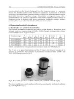
Figure 4.4.11: PD independent joint control.
4.4 Computed-Torque Control
Copyright © 2004 by Marcel Dekker, Inc.

Computed-Torque Control214
(4.4.55)
with the closed-loop characteristic polynomial
(4.4.56)
The PD gains can be selected to obtain a suitable natural frequency and
damping ratio, as we have seen.
At steady state, the only nonzero contribution to the disturbance d(t) is the
neglected gravity G(q). Table 3.3.1 shows that the gravity vector is bounded
by a known value g
b
for a given robot arm. Therefore, at steady state,

Using the final value theorem, the steady-state tracking error for joint i
using PD control is bounded by
(4.4.57)
Therefore, for set-point tracking where a final value for q
d
is specified and
PD control with a large k
p
might be suitable.
As a matter of fact, the next results show that PD control is often very
suitable even for following a desired trajectory, not only for set-point control.
It is proven in [Dawson 1990].
THEOREM 4.4–2: If the PD control law (4.4.54) is applied to each joint and
e(0)=0, (0)=0, the position and velocity tracking errors are bounded within a
ball whose radius decreases approximately (for large k
v
)
as .

᭿
This result gives credence to those who maintain that PD control is often
good enough for practical applications.
Of course, the point is that k
v
cannot be increased without limit without
hitting the actuator torque limits. Other schemes to be discussed in the book
allow good trajectory following without such large torques.
In [Paul 1981] are discussed several methods for modifying the PD control
law to obtain better performance. These include gravity compensation [which
yields exactly controller (4.4.49)], and acceleration feedforward, which
amounts to using
(4.4.58)
Copyright © 2004 by Marcel Dekker, Inc.
215
for each joint. Also mentioned is joint-coupling control, which amounts to
adding back into u(t) some of the neglected terms in M(q) and N(q, )that
describe the interactions between the joints. Thus such corrections involve
using better estimates for and in the approximate computed-torque
control (4.4.43).
PID Control. It has been seen that PD independent joint control is often suitable
for tracking control. However, at steady state there is a residual error (4.4.57)
due to gravity. This can be removed using the PID independent joint control
law
(4.4.59)
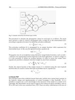
for each joint. See Figure 4.4.12.
4.4 Computed-Torque Control
Now the transfer function for set-point tracking is
(4.4.60)
with closed-loop characteristic polynomial

(4.4.61)
Now the final value theorem shows that the steady-state error for set-point
control is zero. The Routh test shows that for stability it is required that
Figure 4.4.12: PID independent joint control.
Copyright © 2004 by Marcel Dekker, Inc.