Robot Manipulator Control Theory and Practice - Frank L.Lewis Part 8 pptx

Robust Control of Robotic Manipulators268
of q for robots with prismatic joints, and that (5.2.10) is satisfied by
so that a=(µ
2
-
µ
1
)/(µ
2
+µ
1
)) [Spong and Vidyasagar 1987]. Finally, (5.2.10) is a result of the
properties of the Coriolis and centripetal terms discussed in Section 3.3.
We will give different representative designs of the feedback-linearization
approach, starting with controllers whose behavior is studied using Lyapunov
stability theory.
Lyapunov Designs
Static feedback compensators have been extensively used starting with the
works of [Freund 1982] and [Tarn et al. 1984]. Consider the controller
introduced in (4.4.13):
(5.2.12)
such that
(5.2.13)
It can be seen that by placing the poles of A
c
sufficiently far in the left half-
plane, the robust stability of the closed- loop system in the presence of
␩
is
guaranteed. This was shown true in [Arimoto and Miyazaki 1985] for the

case where as described in Theorem 4.4.1 and Example
4.4.3. It was also shown true for the trajectory-following problem assuming
that in [Dawson et al. 1990] as described in Theorem 4.4.2.
There are as many robust controllers designed using Lyapunov stability
concepts as there are ways of choosing Lyapunov function candidates, and
of designing the gain K to guarantee that the Lyapunov function candidate is
decreasing along the trajectories of (5.2.13). To decrease the asymptotic
trajectory error, however, excessively large gains may be required (see Example
4.4.3). We therefore choose to use the passivity theorem and a choice of the
gain matrix K that renders the linear part of the closed-loop system SPR. As
described in Section 2.11, an output may be chosen to make the closed-loop
system SPR; therefore allowing large passive uncertainties in the knowledge
of M(q). In fact, the state-feedback controller may be used to define an
appropriate output Ke such that the input-output closed-loop linear systems
K(sI-A+BK)
-1
B is strictly positive real (SPR). Consider the following closed-
loop linear system:
Copyright © 2004 by Marcel Dekker, Inc.
269
(5.2.14)
It may then be shown using Theorem 2.11.5 that this system is SPR if
(5.2.15)
with the choice of
(5.2.16)
such that
(5.2.17)
is the positive-definite solution to the Lyapunov equation
(5.2.18)
and

(5.2.19)
The next theorem presents sufficient conditions for the uniform boundedness
of the trajectory error.
THEOREM 5.2–1: The closed-loop system given by (5.2.13) will be uniformly
bounded if

and
where K
v
=2aI and K
p
=4aI.
Proof:
5.2 Feedback-Linearization Controllers
Copyright © 2004 by Marcel Dekker, Inc.
Robust Control of Robotic Manipulators270
Consider the closed-loop system given by (5.2.8), with the controller
(5.2.12), and choose the following Lyapunov function candidate:
(1)
where
is the Lyapunov function corresponding to the SPR system
(5.2.14). Then if ⌬≥0, we have that V>0. This condition is satisfied for ≥µ
2
I.
Then differentiate to find
(2)
To guarantee that V < 0 recall the bounds (5.2.8)–(5.2.11), and write
(3)
where
. Note that ||e|| may be factored out of (3) without affecting

the sign definiteness of the equation. The uniform boundedness of the error
is then guaranteed using Lemma 2.10.3 and Theorem 2.10.3 if
(4)
which is guaranteed if
(5)
or
(6)
The error will be bounded by a term that goes to zero as a increases (see
Theorem 2.10.3 and its proof in [Dawson et al. 1990] for details). This
analysis then allows ⌬ to be arbitrarily large as long as ≥µ
2
I, as shown in
the next example. In fact, if N were known, global asymptotic stability is
assured from the passivity theorem since in that case ␦=0. The controller is
It is instructive to study (6) and try to understand the contribution of
each of its terms. The following choices will help satisfy (6).
1. Large gains K
p
and K
v
which correspond to a large a.
᭿
Copyright © 2004 by Marcel Dekker, Inc.
summarized in Table 5.2.1.
271
2. A good knowledge of N which translates into small
␤
i
’s.
3. A large µ

1
or a large inertia matrix M(q).
4. A trajectory with a small c, this a small desired acceleration
d
.
Figure 5.2.2: K
p
=50, K
v
=25 (a) errors of joint 1; (b) errors of joint 2; (c) torques of
joints 1 and 2.
The following example illustrates the sufficiency of condition (6) and of the
effects of larger gains K
p
and K
v
.
5.2 Feedback-Linearization Controllers
Copyright © 2004 by Marcel Dekker, Inc.
Robust Control of Robotic Manipulators272
(1)
where
EXAMPLE 5.2–1: Static Controller (Lyapunov Design)
In all our examples in this chapter we use the two-link revolute-joint robot
first described in Chapter 3, Example 3.2.2, whose dynamics are repeated
here:
(2)
The parameters m
1
=1kg, m

2
=1kg, a
1
=1m, a
2
=1m, and g=9.8 m/s
2
are given.
Let the desired trajectory used in all examples throughout this chapter be
described by
Then . It may then be shown that

Let =0 then
or that
Then use =6I and a=172 to satisfy (6). In fact, these values will lead to a
larger controller gains than are actually needed. Suppose instead that we let
6
^
I, =0, and that
Copyright © 2004 by Marcel Dekker, Inc.
273
(3)
Note that this is basically a computed-torque-like PD controller. A simulation
of the robot’s trajectory is shown in Figure 5.2.2. We also start our simulation
at =0. The effect of increasing the gains is shown in Figure 5.2.3,
which corresponds to the controller
(4)
Note that at least initially, more torque is required for the higher-gains case
(compare Figs. 5.2.2c and 5.2.3c) but that the errors magnitude is greatly
reduced by expanding more effort.

There are other proofs of the uniform boundedness of these static controllers.
In particular, the results in [Dawson et al. 1990] provide an explicit expression
for the bound on e in terms of the controller gains. In the interest of brevity
and to present different designs, we choose to limit our development to one
controller in this section.
As discussed in Section 4.4, a residual stead-state error may be present
even when using an exact computed-torque controller if disturbances are
present. A common cure for this problem (and one that will eliminate constant
disturbances) is to introduce integral feedback as done in Section 4.4. Such a
controller may again be used within a robust controller framework and will
lead to similar improvements if the integrator windup problem is avoided
(see Section 4.4).
In the next section we show the stability of static controllers similar to the
ones designed here and use input-output stability methods to design more
general dynamic compensators.
Input-Output Designs
In this section we group designs that show the stability of the trajectory
error using input-output methods. In particular, we present controllers that
show
∞
and
2
stability of the error. We divide this section into a subsection
that deals with static controllers such as the ones described previously,
᭿
5.2 Feedback-Linearization Controllers
Copyright © 2004 by Marcel Dekker, Inc.
Robust Control of Robotic Manipulators276
the error signals was shown using a static controller. The norms used in
(5.2.8)–(5.2.10) are then

∞
norms. The development of this controller starts
with assumptions (5.2.8), (5.2.9), and a modification of (5.2.10) to
(5.2.20)
This assumption is justified by the fact that N is composed of gravity and
velocity-dependent terms which may be bounded independent from the
position error e [see (5.1.1)]. We shall also assume that
=0. Let us
then choose the state-feedback controller (5.2.12) repeated here for
convenience:
(5.2.21)
The corresponding input-output differential equation
(5.2.22)
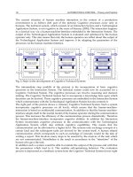
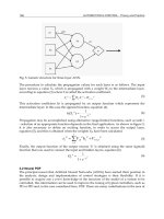
A block diagram description of this equation is given in Figure 5.2.4. Consider
now the transfer function from
η
(taken as an independent input) to e:
(5.2.23)
or
(5.2.24)
It can be seen that K
v
and K
p
are both diagonal, with , a critically
damped response it achieved at every joint [see (4.4.22), (4.4.30), and
(3.3.32)]. The infinity operator gains of P
11
(s) and P
12

(s) are (see Lemma
2.5.2 and Example 2.5.8)
(5.2.25)
where
(5.2.26)
Consider then the following inequalities:
Copyright © 2004 by Marcel Dekker, Inc.
277
and using (5.2.8)–(5.2.11), we have that
(5.2.27)
The following theorem presents sufficient conditions for the boundedness of
the error that parallel those of Theorem 5.2.1.
THEOREM 5.2–2: Suppose that
and
(1)
Then the
∞
stability of the error is guaranteed if
(2)
Proof:
The condition above results from applying the small-gain theorem to the
closed-loop system, under the assumption that e(0)=0 so that the quadratic
term ||e||
2
is small. See [Craig 1988] for details.
Note that (2) reduces to
and further to
(5.2.28)
Let us study the inequality above to determine the effect of each term. The
following observations are made to help satisfy (5.2.28).

1. A large k
v
will help satisfy the stability condition. Note: That will also
imply a large k
p
.
5.2 Feedback-Linearization Controllers
Copyright © 2004 by Marcel Dekker, Inc.
Robust Control of Robotic Manipulators278
2. A good knowledge of N, which will translate into small
␤
i
’s.
3. A large µ
1
or a large inertia matrix M(q).
4. A trajectory with a small
d
.
5. Robots whose inertia matrix M(q) does not vary greatly throughout its
workspace (i.e. µ
1
≈µ
2
)), so that a is small. Note that a small a is needed
to guarantee that at least < 1 in (5.2.28). This will translate into
the severe requirement that the matrix M should be close to the inertia
matrix M(q) in all configurations of the robot.
The controller is summarized in Table 5.2.2.
These observations are similar to those made after inequality (6) and are

illustrated in the next example.
EXAMPLE 5.2–2: Static Controller (Input-Output Design)
Consider the nonlinear controller (5.2.6), where
(1)
Therefore,
(2)
Condition (1) is then satisfied if k
v
>720. This of course is a large bound that
can be improved by choosing a better . A simulation of the closed-loop
behavior for k
p
=225 and k
v
=30 is shown in Figure 5.2.5. The errors
magnitudes are much smaller than those achieved with the PD controllers of
Example 5.2.1 with a comparable control effort. This improvement came
with the expense of knowing the inertia matrix M(q) as seen in (1).
Dynamic Controllers
The controllers discussed so far are static controllers in that they do not
have a mechanism of storing previous state information. In Chapter 4 and in
this chapter, these controllers could operate only on the current position and
velocity errors. In this section we present three approaches to show the
robustness of dynamic controllers based on the feedback-linearization
᭿
Copyright © 2004 by Marcel Dekker, Inc.
281
(5.2.31)
and let the operator gains of P
i

, i=1,2, be given by
(5.2.32)
Note that ␥
1
=max ␥
11
, ␥
12
. See Lemma 2.5.2 and Example 2.5.8. Consider
then
(5.2.33)
The next theorem gives sufficient conditions for the BIBO stability of the
trajectory error.
THEOREM 5.2–3: The BIBO stability of the closed-loop system (5.2.30)
will be guaranteed if
(1)
In fact, the trajectory error is bounded by
(2)
Proof:
By the small-gain theorem. See [Spong and Vidyasagar 1987] for
details.
If we study (1) carefully we note that it will be satisfied if
1. µ
1
is large or M(q) is large.
2. Good knowledge of N, resulting in a small
␤
1
.
3. Small ␥

1
due to a large gain of the compensator C.
5.2 Feedback-Linearization Controllers
᭿
Copyright © 2004 by Marcel Dekker, Inc.
Robust Control of Robotic Manipulators282
4. ␥
2
close to 1, which may also be obtained with a large-gain compensator
C.
Note that in the limit, and as the gain of C(s) becomes infinitely large, ␥
1
goes to zero. This will then transform condition (1) to
(5.2.34)
It is also seen from (5.2.33)–(5.2.34) that increasing the gain k of C(s) will
decrease ␥
1
, therefore decreasing ||e||
∞
. A particular compensator may now
be obtained by choosing the parameter Q(s) to satisfy other design criteria,
such as suppressing the effects of
␩
. One can, for example, recover Graig’s
compensator, by choosing C(s)=-K so that the control effort is given by
u=Ke. (5.2.35)
Then note that conditions (5.2.28) and (1) are identical if
␤
2
=0 and

␥
2
=
␥
11
k
p
+
␥
12
k
v
. Also note from (2) that a smaller
d
results in a smaller tracking
error. In fact, if
e
=0 and
␤
0
=0, the asymptotic stability of the error may be
shown. Finally, note that the presence of bounded disturbance will make the
bound on the error e larger but will not affect the stability condition (1).
This controller is summarized in Table 5.2.3.
The factorization approach gives the family of all one-degree-of-freedom
stabilizing compensators C(s). The design methodology is illustrated for the
two-link robot in the next example.
EXAMPLE 5.2–3: Dynamic Controller (Input-Output Design)
Let G
v

(s) of Example 4.2.1 be factored as
(1)
where N(s), D(s), N(s), and D(s) are matrices of stable rational functions.
We can then find
(2)
Copyright © 2004 by Marcel Dekker, Inc.
Robust Control of Robotic Manipulators284
(3)
Then all the stabilizing controllers are given by
(4)
where Q(s) is a stable rational function which is otherwise arbitrary. One
choice, of course, is to let Q(s)=0, which leads to the “central solution”
[Vidyasagar 1985]
(5)
One can also choose Q(s) to satisfy the required performance. In particular,
the following choice of Q(s) is presented in [Spong and Vidyasagar
1987]:
(6)
which leads to the following controller:

where
and
(7)
As k increases, the disturbance rejection property of the controller is enhanced
at the expense of higher gains as seen from the expression of C(s). A simulation
Copyright © 2004 by Marcel Dekker, Inc.
285
of this controller for k=225 is shown in Figure 5.2.6. The following
observations are in order: The trajectory errors are smaller than any of the
previous controllers while the torque efforts are comparable. In addition,

the complexity of the controller is acceptable since the dynamics of the robot
are not used in implementing the control.
Figure 5.2.6: (a) errors of joint 1; (b) errors of joint 2; (c) torques of joints 1
and 2.
As it was discussed in [Craig 1988] and presented in Theorem 5.2.2,
including the more reasonable quadratic bound will not destroy the
∞
᭿
5.2 Feedback-Linearization Controllers
Copyright © 2004 by Marcel Dekker, Inc.
Robust Control of Robotic Manipulators286
stability result of [Spong and Vidyasagar 1987]. It was shown in [Becker
and Grimm 1988], however, that the
2
stability of the error cannot be
guaranteed unless the problem is reformulated and more assumptions are
made. It effect, the error will be bounded, but it may or may not have a finite
energy. In particular, noisy measurements are no longer tolerated for
2
stability to hold. We next present an extension of the
∞
stability result that
applies to dynamical compensators similar to the one described in Theorem
5.2.3 but without the requirement that
␤
2
=0.
THEOREM 5.2–4: The error system of (5.2.30) is
∞
bounded if

=0
and
(1)
Proof:
An extension of the small-gain theorem. See [Becker and Grimm 1988]
for details.
A study of (1) reveals that the following desired characteristics will help
satisfy the inequality:
1. A large µ
1
due to a large M(q).
2. A small ␥
1
and a ␥
2
close to 1, which will result from a large-gain
compensator C.
3. Small
␤
i
’s, which will result from a good knowledge of N.
4. A small c due to a small
d
.
Note that Craig’s conditions in Theorem 5.2.2 are recovered if ␥
1
=max ␥
11
,
␥

12
and ␥
2
k=␥
11
k
p
+␥
12
k
v
.
On the other hand, assuming that
d
=0 and
␤
2
=0, the
2
stability of e was
shown in [Becker and Grimm 1988] if
(5.2.36)
where as given in Lemma 2.5.2. This
controller is summarized in Table 5.2.4.
᭿
Copyright © 2004 by Marcel Dekker, Inc.
Robust Control of Robotic Manipulators288
is due to the fact that the velocity terms are truly negligent in this particular
application. Such terms will, however, make a more vital contribution in
faster trajectories.

Figure 5.2.7: (a) errors of joint 1; (b) errors of joint 2; (c) torques of joints 1
and 2.
Two-Degree-of-Freedom Design.
It is well known that the two-DOF structure is the most general linear
controller structure. The two-DOF design allows us simultaneously to specify
the desired response to a command input and guarantee the robustness of
᭿
Copyright © 2004 by Marcel Dekker, Inc.
289
the closed-loop system. This design was briefly discussed in Chapter 2,
Example 2.11.4. It is in a different spirit from the other design of this chapter,
because it relies on classical frequency-domain SISO concepts. The general
structure is shown in Figure 5.2.8. A two-DOF robust controller was designed
and simulated in [Sugie et al. 1988] and will be presented next. Let the plant
be given by (5.2.5) and consider the following factorization:
G(s)=N(s)D
-1
(s),
where
D(s)=s
2
, N(s)=I. (5.2.37)
The following result presents a two-DOF compensator which will robustly
stabilize (in the
∞
sense) the error system.
THEOREM 5.2–5: Consider the two-DOF structure of Figure 5.2.8. Let
K
1
(S) be a stable system and K

2
(s) be a compensator to stabilize G(s). Then
the controller
u=s
2
K
1
v+K
2
(K
1
v-q) (1)
will lead to the closed-loop system
q=K1v (2)
and the closed-loop error system (5.2.13) will be
∞
stable.
Proof:
With simple block-diagram manipulations, it may be shown that the closed-
loop system is
q=K
1
v.
The actual robustness analysis is involved and will be omitted, but a particular
design and its robustness are discussed in the next example.
Note from (2) that K
1
(s) is used to obtain the desired closed-loop transfer
function. It should then be stable, and to guarantee a zero steady-state error,
we choose v=qd and make sure that the dc gain K

1
(0)=1. Finally, we would
like K
1
(S) to be exactly proper (i.e., zero relative degree). K
2
(s), on the other
hand, will assure the robustness of the closed-loop system. Therefore, K
2
(s)
should stabilize G(s) and provide suitable stability margins. It should contain
5.2 Feedback-Linearization Controllers
᭿
Copyright © 2004 by Marcel Dekker, Inc.
291
or
(3)
We can immediately see that the joint position vector q is filtered through
the PID controller K
2
. Therefore, the differentiation of q is required unless
the measurement of is available. The behavior of the nonlinear closed-loop
system is shown in Figure 5.2.9, when
=1 and =0, a
1
=2, b
1
=b
2
=10, w

1
=8,
and w
2
=12. It is seen that initially, the torque effort and the trajectory errors
are too large. To understand the behavior of this controller, consider the
controller
τ
in the limit (i.e., as time goes to infinity). The output of K
1qd
has
settled down to its final value qd and therefore the controller (3) becomes
equivalent to a PID compensator [see Chapter 4, equation (4.4.35)]. It seems
that a different structure for k
1
and K
2
is warranted because in the meantime,
the two-DOF controller preforms rather poorly. This is a characteristic of
the example rather than an inherent flow in the twoDOF methodology. As a
matter of fact, this structure has shown better performance than the one-
DOF PID compensator in [Sugie et al. 1988] for a set-tracking case. The
reader is encouraged to work the problems at the end of the chapter related
to this design in order to compare the performance of one- and two-DOF
designs.
We have this presented a large sample of controllers that are more or less
computed-torque based. We have shown using different stability arguments
that the computed-torque structure is inherently robust and that by
increasing the gains on the outer-loop linear compensator, the position and
velocity errors tend to decrease in the norm. This class of compensators

constitutes by far the most common structure used by robotics
manufacturers and is the simplest to implement and study. There are more
compensators that would fit into this structure while appealing to some
classical control applications. The PD and PID compensators may be
replaced with the lead-lag compensators. These are especially appealing
when only position measurements are available. Such designs are discussed
in [Chen 1989] in the discrete-time case. There is also some work being done
in the nonlinear observer area which is directly relevant to this problem
[Canudas de Wit and Fixot 1991]. We refer the reader to the observability
discussion in Section 2.11. We also suggest some of the problems at the end
of this chapter, which discuss further modification of the feedback-
linearization designs.
᭿
5.2 Feedback-Linearization Controllers
Copyright © 2004 by Marcel Dekker, Inc.
293
5.3 Nonlinear Controllers
There is a class of robot controllers that are not computed-torque-like
controllers. These controllers are obtained directly from the robot equations
without using the feedback-linearization procedure. Instead, these controller
may rely on other properties of the robot (such as the passivity of its Lagrange-
Euler description) or may be obtained without even considering the physics
of the robot. In general, these controllers may be written as a computed-
torque controller with an auxiliary, nonlinear controller added to it. The
nonlinear control term introduces coupling between the different joints
independently from the computed-torque term. In other words, even if the
computed-torque controller is a simple PID, the nonlinear term couples all
joints together as will be seen in Theorems 5.3.4 and 5.3.5, for example.
Direct Passive Controllers
First, we present controllers that rely directly on the passive structure

of rigid robots as described in equations (5.1.1), where (q)-2V
m
(q, )
is skew symmetric by an appropriate choice of V
m
(q, ) as described in
Section 3.3.
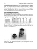
Based on the passivity property, if one can close the loop from to
␶
with
a passive system (along with
2
bounded inputs) as in Figure 5.3.1, the closed-
loop system will be asymptotically stable using the passivity theorem. Note
that the input u
2
gives an extra degree of freedom to satisfy some performance
criteria. In other words, by choosing different
2
bounded u
2
we may be able
to obtain better trajectory tracking or noise immunity. This structure will
show the asymptotic stability of but only the Lyapunov stability of e. On
Figure 5.3.1: Passive-control structure.
5.3 Nonlinear Controllers
Copyright © 2004 by Marcel Dekker, Inc.
Robust Control of Robotic Manipulators294
the other hand, if one can show the passivity of the system, which maps
␶

to
a new vector r which is a filtered version of e, a controller that closes the
loop between -r and
␶
will guarantee the asymptotic stability of both e and .
This indirect use of the passivity property was illustrated in [Ortega and
Spong 1988] and will be discussed first.
Let the controller be given by (5.3.1), where F(s) is a strictly proper, stable,
rational function, and K
r
is a positive-definite matrix,
(5.3.1)
Substituting (5.3.1) into (5.1.1) and assuming no friction [i.e., F( )=0], we
obtain
(5.3.2)
Then it may be shown that both e and are asymptotically stable. In fact,
choose the following Lyapunov function:
Then
Substituting for M(q) from (5.3.2), we obtain
Therefore, r is asymptotically stable, which can be used to show that both e
and e are asymptotically stable [Slotine 1988]. This approach was used in
the adaptive control literature to design passive controllers [Ortega and Spong
1988], but its modification in the design of robust controllers when M, V
m
and G are not exactly known is not immediately obvious. Such modifications
will be given in the variable-structure designs, but first, we present a simple
controller to illustrate the robustness of passive compensators.
Copyright © 2004 by Marcel Dekker, Inc.
295
THEOREM 5.3–1: Consider the control law (1)

(1)
where ⌳(s) is an SPR transfer function, to be chosen by the designer, and the
external input u
2
is bounded in the
2
norm. Then is asymptotically stable,
and e is Lyapunov stable.
Proof:
Using the control law above, one gets from Figure 5.3.1,
(2)
By an appropriate choice of ⌳(s) and u
2
, one can apply the passivity theorem
and deduce that and r are bounded in the
2
norm, and since ⌳(s)
-1
is SPR
(being inverse of an SPR function), one deduces that is asymptotically
stable because
(3)
This will imply that the position error e is bounded but not its asymptotic
stability in the case of time-varying trajectories . In the set-point
tracking case, however (i.e.,
d
=0), and with gravity precompensation, the
asymptotic stability of e may be deduced using LaSalle’s theorem. The
robustness of the closed-loop system is guaranteed as long as ⌳(s) is SPR
and that u

2
is
2
bounded, regardless of the exact values of the robot’s
parameters.
The controller is summarized in Table 5.3.1.
Table 5.3.1: Passive Controller
5.3 Nonlinear Controllers
᭿
Copyright © 2004 by Marcel Dekker, Inc.
Robust Control of Robotic Manipulators296
EXAMPLE 5.3–1: Passive Controllers
We choose an SPR transfer function
(1)
and we let u
2
=
d
. Note that the desired trajectory used so far violates the
assumption that u
2
should be
2
stable. Nevertheless, the trajectories of
Figure 5.3.2: (a) errors of joints 1; (b) errors of joint 2; (c) torques of joints 1
and 2.
Copyright © 2004 by Marcel Dekker, Inc.
297
Figure 5.3.2 show that his controller, when started at e(0)= (0)=0, performs
rather well for the sinusoidal trajectory. Of course, since the passivity theorem

provides sufficient conditions for stability, this example is not contradicting
the previous theorem but merely pointing out its conservatism.
Note that the compensator of Theorem 5.3.1 is a generalization of the PD
compensators of Chapter 4 and of the preceding section. In [Anderson 1989]
it was demonstrated, using network-theoretic concepts, that even in the
absence of the contact forces, a computed-torque-like controller is not passive
and may therefore cause instabilities in the presence of uncertainties. His
solution to the problem consisted of using proportionalderivative (PD)
controllers with variable gains K
1
(q) and K
2
(q) which depend on the inertia
matrix M(q), that is,
(5.3.3)
Even though M(q) is not exactly known, the stability of the closed-loop
error is guaranteed by the passivity of the robot and the feedback law. The
advantage of this approach is that contact forces and larger uncertainties
may now be accommodated. Its main disadvantage is that although robust
stability is guaranteed, the closed-loop performance depends on the
knowledge of M(q), whose singular values are needed in order to find K
p
and K
v
. We will not discuss this particular design and refer the interested
reader to [Anderson 1989].
Variable-Structure Controllers
In this section we group designs that use variable-structure (VSS) controllers.
The VSS theory has been applied to the control of many nonlinear processes
[DeCarlo et al. 1988]. One of the main features of this approach is that one

only needs to drive the error to a “switching surface,” after which the system
is in “sliding mode” and will not be affected by any modelling uncertainties
and/or disturbances.
There are two main criticisms of these controllers as they apply to robots.
The first is that by ignoring the physics or the robot, these controllers will
necessarily perform no better (if not worse) that controllers which exploit
the structure of the Lagrange-Euler equations. The other criticism relates to
the “chattering” problem commonly associated with variable-structure
controllers. We shall address the second issue later in this section, and answer
the first by admitting that although initial applications of variable-structure
theory did indeed gloss over the physics of robots, later designs (such as the
5.3 Nonlinear Controllers
᭿
Copyright © 2004 by Marcel Dekker, Inc.
Robust Control of Robotic Manipulators298
ones discussed here) by [Slotine 1985] and [Chen et al. 1990] remedied the
problem.
The first application of this theory to robot control seems to be in [Young
1978], where the set-point regulation problem (
d
=0)was solved using the
following controller:
(5.3.4)
where i=1,…, n for an n-link robot, and r
i
are the switching planes,
(5.3.5)
It is then shown, using the hierarchy of the sliding surfaces r
1
, r

2
,…, r
n
and
given bounds on the uncertainties in the manipulators model, that one can
find
␶
+
and
␶
-
in order to drive the error signal to the intersection of the
sliding surfaces, after which the error will “slide” to zero. This controller
eliminates the nonlinear coupling of the joints by forcing the system into the
sliding mode. Other VSS robot controllers have since been designed.
Unfortunately, for most of these schemes, the control effort as seen from
(5.3.4) is discontinuous along r
i
=0 and will therefore create chattering, which
may excite unmodelled high-frequency dynamics. In addition, these
controllers do not exploit the physics of the robot and are therefore less
effective than controllers that do.
To address this problem, the original VSS controllers were modified in
[Slotine 1985] as described in the next theorem. Let us first define a few
variables to simplify the statement of the theorem. Let
(5.3.6)
where
THEOREM 5.3–2: Consider the controller
Copyright © 2004 by Marcel Dekker, Inc.
299

where

Then the error reaches the surface
in a finite time. In addition, once on the surface, q(t) will go to q
d
(t)
exponentially fast.
Proof:
Consider the Lyapunov function candidate
Then
Substituting for and using the skew-symmetric property of (q)-2V
m
(q, )
we obtain
Then, if we use the controller given by
we obtain
where
5.3 Nonlinear Controllers
Copyright © 2004 by Marcel Dekker, Inc.