Robot Motion Planning and Control - J.P. Laumond Part 12 ppt
Bạn đang xem bản rút gọn của tài liệu. Xem và tải ngay bản đầy đủ của tài liệu tại đây (2.25 MB, 25 trang )
268 P. ~vestka and M. H. Overmars
processor running at 150 MHZ. This machine is rated with 96.5 SPECfp92 and
90.4 SPECint92.
In the test scenes used, the coordinates of all workspace obstacles lie in the
unit square. Furthermore, in all scenes we have added an obstacle boundary
around the unit square, hence no part of the robot can move outside this square.
The experiments are aimed at measuring the "knowledge" acquired by the
method after having constructed roadmaps for certain periods of time. This is
done by testing how well the method solves certain (interesting) queries. For
each scene S we define a
query test set TO. =
{(sl, sl),
(s2,g2), ,
(sra,gm)},
consisting of a number of configuration pairs (that is, queries). Then, we re-
peatedly construct a graph for some specified time t, and we count how many
of these graphs solve the different queries in
TQ.
This experiment is repeated
for a number of different construction times t. The results are presented in the
tables under the figures. The numbers in the boxes indicate the percentage of
the runs that solve the corresponding query within the given time bound.
The values for the random walk parameters
Nw
and
Lw
are, respectively,
10 and 0.05. This guarantees that the time spent per query is bounded by
approximately 0.3 seconds (on our machine). Clearly, if we allow more time per
query, the method will be more successful in the query phase, and vice versa.
Hence there is a trade-off between the construction time and the time allowed
for a query.
In Figure 1 we have a free flying L-shaped robot, placed at the configurations
a, b, and c. Simulation results are shown for the three corresponding queries,
and two paths are shown, both smoothed in 1 second. We see that around 1
second of roadmap construction is required for obtaining roadmaps that solve
the queries. These roadmaps consist of approximately 125 nodes.
In Figures 2 to 4 results are given for articulated robots.
In the first two scenes, just one query is tested, and well the query (a, b).
In both figures, several robot configurations along a path solving the query are
displayed using various grey levels. The results of the experiments are given
in the two tables. We see that the query in Figure 2 is solved in all cases
after 10 seconds of construction time. Roadmap construction for 5 seconds
however suffices to successfully answer the query in more than 90% of the
cases. In Figure 3 we observe something similar. For both scenes the roadmaps
constructed in 10 seconds contain around 500 nodes.
Figure 4 is a very difficult one. We have a seven dof robot in a very con-
strained environment. The configurations a, b, c, and d define 6 different queries,
for which the results are shown. These where obtained by a customised imple-
mentation by Kavraki et al. [23]. In this implementation, optimised collision
Probabilistic Path Planning 269
Fig. 1. An L-shaped free-flying robot and its test configurations are shown. At the
top right, we see two paths computed by the planner and smoothed in 1 second.
Fig. 2. A four dof articulated robot, and a path.
270 P. Svestka and M. H. Overmars
Fig. 3. A five dof articulated robot, and a path.
checking routines are used, as well as a robot-specific local planner. ~rther-
more, "difficult" nodes are heuristically identified during the roadmap construc-
tion phase, and "expanded" subsequently. We see that roughly 1 minute was
sufficient to obtain roadmaps solving the 6 queries. These roadmaps consist of
approximately 4000 nodes.
4 Application to nonholonomic robots
In this section we deal with nonholonomic mobile robots. More specifically, we
apply
PPP
to car-like robots and tractor-trailer robots. We consider two types
of car-like robots, i.e., such that can drive both forwards and backwards, and
such that can only drive forwards. We refer to the former as
general car-like
robots,
and to the latter as
forward car-like robots.
First however we give a brief
overview on previous work on nonholonomic motion planning.
4.1 Some previous work on nonholonomic motion planning
Nonholonomic constraints add an extra level of difficulty to the path planning
problem. The paths must (1) be collision free and (2) describe motions that
are executable for the robot. We refer to such paths as
feasible
paths.
Probabilistic Path Planning 271
Fig. 4. A seven dof articulated robot in a very constrained environment and the query
test set.
For
locally controllable robots
[6], the existence of a feasible path between
two configurations is equivalent to the existence of a collision free path, due to
the fact that for any collision free path there exists a feasible path lying arbi-
trarily close to it. This fundamental property has led to a family of algorithms,
decomposing the search in two phases. They first try to solve the geometric
problem (i.e., the problem for the holonomic robot that is geometrically equiv-
alent to the nonholonomic one). Then they use the obtained collision-free path
to build a feasible one. So in the first phase the decision problem is solved,
and only in the second phase are the nonholonomic constraints taken into ac-
count. One such approach was developed for car-like robots [26], using Reeds
and Shepp works on optimal control to approximate the geometric path. In [34]
Reeds and Shepp presented a finite family of paths composed of line segments
and circle arcs containing a length-optimal path linking any two configurations
(in absence of obstacles). The planner introduced in [26] replaces the collision-
free geometric path by a sequence of Reeds and Shepp paths. This complete
and fast planner was extended to the case of tractor-trailer robots, using near
optimal paths numerically computed [27,12] (so far the exact optimal paths
for the tractor-trailer system in absence of obstacle are unknown). The result-
ing planners are however neither complete nor time-efficient. The same scheme
was used for systems that can be put into the
chained form.
For these sys-
tems, Tilbury et al. [50] proposed different controls to steer the system from
272 P. ~vestka and M. H. Overmars
one configuration to another, in absence of obstacles. Sekhavat and Laumond
prove in [38] that the sinusoidal inputs proposed by Tilbury et al. can be used
in a complete algorithm transforming any collision-free path to a feasible one.
This algorithm was implemented for a car-like robot towing one or two trail-
ers, which can be put into the chained form, and finds paths in reasonable
times [38]. A multi-level extension of this approach has been presented in [40]
which further improves the running times of this scheme by separating the
nonholonomic constraints mutually, and introducing separately. The scheme
is however, as pointed out, only applicable to locally controllable robots. For
example, forward car-like robots do not fall in this class.
Barraquand and Latombe [6] have proposed a heuristic brute-force approach
to motion planning for nonholonomic robots. It consists of heuristically build-
ing and searching a graph whose nodes are small axis-parallel cells in C-space.
Two such cells are connected in the graph if there exists a basic path between
two particular configurations in the respective cells. The completeness of this
algorithm is guaranteed up to appropriate choice of certain parameters, and it
does not require local controllability of the robot. The main drawback of this
planner is that when the heuristics fail it requires an exhaustive search in the
discretised C-space. Furthermore, only the cell containing the goal configura-
tion is reached, not the goal configuration itself. Hence the planner is inexact.
Nevertheless, in many cases the method produces nice paths (with minimum
number of reversals) for car-like robots and tractors pulling one trailer. For sys-
tems of higher dimension however it becomes too time consuming. Ferbach [11]
builds on the approach of Barraqua.nd and Latombe method in his progressive
constraints algorithm in order to solve the problem in higher dimensions. First
a geometric path is computed. Then the nonholonomic constraints are intro-
duced progressively in an iterative algorithm. Each iteration consists of explor-
ing a neighbourhood of the path computed in the previous iteration, searching
for a path that satisfies more accurate constraints. Smooth collision-free paths
in non-trivial environments were obtained with this method for car-like robots
towing two and three trailers. The algorithm however does not satisfy any form
of completeness.
The probabilistic path planner PPP has been applied to various types of
nonholonomic robots. An advantage over the above single shot methods is the
fact that a roadmap is constructed just ones, from which paths can subse-
quently be retrieved quasi-instantaneously. Also, local robot controllability is
not required. A critical point of PPP when applied to nonholonomic robots
is however the speed of the nonholonomic local planner. For car-like robots
very fast local planners have been developed. Thanks to this, PPP applied to
the car-like robots resulted in fast and probabilistically complete planners for
car-like robots that move both forwards and backwards, as well as for such
that can only move forwards [45,47]. Local planners for tractor-trailer robots
Probabilistic Path Planning 273
however tend to be much more time-consuming, which makes direct use of PPP
less attractive. In [49] a local planner is presented and integrated into PPP,
that uses exact closed form solutions for the kinematic parameters of a tractor-
trailer robot. In [39] the local planner using sinusoidal inputs for chained form
systems is used. For robots pulling more than one trailer, this local planner ap-
peared to be too expensive for capturing the connectivity of the free C-space.
For this reason, and inspired by the earlier mentioned works [26,27,12,38], in
[39] a two-level scheme is proposed, where at the first level the portion of CSf~ee
is reduced to a neighbourhood of a geometric path, and at the second level a
(real) solution is searched for within this neighbourhood (by PPP). The multi-
level algorithm proposed in [40] can in fact been seen as a generalisation of this
two level scheme.
4.2 Description of the car-like and tractor-trailer robots
We model a car-like robot as a polygon moving in R 2, and its C-space is rep-
resented by R 2 x [0, 27r). The motions it can perform are subject to nonholo-
nomic constraints. It can move forwards and backwards, and perform curves of
a lower bounded turning radius rmi,~, as an ordinary car. A tractor-trailer robot
is modelled as a car-like one, but with an extra polygon attached to it by a
revolute joint. Its C-space is (hence) 4-dimensional, and can be represented by
R 2 x [0, 21r) x [-am~, ama~], where ama~ is the (symmetric) joint bound. The
car-like part (the tractor) is a car-like robot. The extra part (the trailer) is sub-
ject to further nonholonomic constraints. Its motions are (physically) dictated
by the motions of the tractor (For details, see for example [25,40]).
For car-like robots, the paths constructed will be sequences of translational
paths (describing straight motions) and rotational paths (describing motions
of constant non-zero curvature) only. It is a well-known fact [25] that if for a
(general or forward) car-like robot a feasible path in the open free C-space exists
between two configurations, then there also exists one that is a (finite) sequence
of rotational paths. We include translational paths to enable straight motions
of the robot, hence reducing the path lengths. For tractor-trailer robots we will
use paths that are computed by transformation of the configuration coordinates
to the chained form, and using sinusoidal inputs.
4.3 Application to general car-like robots
We now apply PPP, using an undirected graph, to general car-like robots. This
again asks for filling in some of the (robot specific) details that have been left
open in the discussion of the general method.
274 P. ~vestka and M. H. Overmars
Filling in the details
The local planner: A RTR path is defined as the concatenation of a rota-
tional path, a translational path, and another rotational path. Or, in other
words, it is the concatenation of two circular arcs and a straight line seg-
ment, with the latter in the middle. The RTR local planner constructs the
shortest RTR path connecting its argument configurations. Figure 5 shows
two RTR paths. It can easily be proven that any pair of configurations
is connected by a number of RTR paths (See [45] for more details). Fur-
thermore, the RTR local planner satisfies a local topological property that
guarantees probabilistic completeness (See Section 5).
e S •
!
i
el
I
Fig. 5. Two RTR paths for a triangular car-like robot, connecting configurations a
and b.
An alternative to the RTR local planner is to use a local planner that con-
structs the shortest (car-like) path connecting its argument configurations
[34], [42]. Constructing shortest car-like paths is however a relatively ex-
pensive operation, and the construct requires more expensive intersection
checking routines than does the RTR construct. On the other hand, RTR
paths will, in general, be somewhat longer than the shortest paths, and,
hence, they have a higher chance of intersection with the obstacles.
Collision checking for a RTR path can be done very efficiently, perform-
ing three intersection tests for translational and rotational sweep volumes.
These sweep volumes are bounded by linear and circular segments (such
objects are also called generalised polygons) and hence the intersection tests
can be done exactly and efficiently. Moreover, the intersection tests for the
Probabilistic Path Planning 275
rotational path segments can be eliminated by storing some extra informa-
tion in the graph nodes, hence reducing the collision check of a RTR path
to one single intersection test for a polygon.
The distance measure: We use a distance measure that is induced by the
RTR local planner, and can be regarded as an approximation of the (too
expensive) induced "sweep volume metric", as described in Section 2.1. The
distance between two configurations is defined as the length (in workspace)
of the shortest RTR path connecting them. We refer to this distance mea-
sure as the
RTR distance measure,
and we denote it by
DRTR.
The random walks in the query phase: Random walks, respecting the
car-like constraints, are required. The (maximal) number of these walks
(per query) and their (maximal) lengths are parameters of the method,
which we again denote by, respectively,
Nw
and
Lw.
Let cs be the start configuration of a random walk. As actual length
Iw
of
the walk we take a random value from [0,
Lw].
The random walk is now
performed in the following way: First, the robot is placed at configuration
cs, and a random steering angle ¢ and random velocity v are chosen. Then,
the motion defined by (¢, v) is performed until either a collision of the
robot with an obstacle occurs, or the total length of the random walk has
reached
Iw. In
the former case, a new random control is picked, and the
process is repeated. In the latter case, the random walk ends.
Good values for
Nw
and
Lw
must be experimentally derived (the values
we use are given in the next section).
Node adding heuristics: We use the geometry of the workspace obstacles
to identify areas in which is advantageous to add some extra, geometri-
cally derived, non-random nodes. Particular obstacle edges and (convex)
obstacle corners define such geometric nodes (See [47] for more details).
Furthermore, as for free-flying robots, we use the (run-time) structure of
the graph G in order to guide the node generation.
Simulation results We have implemented the planner as described above,
and some simulation results are presented in this section. The planner was run
on a machine as described in Section 3. Again the presented scenes correspond
to the unit square with an obstacle boundary, and the chosen values for
Nw
and
Lw
are, respectively, 10 and 0.05. The simulation results are presented in
the same form as for the holonomic robots in Section 3. That is, for different
roadmap construction times we count how often graphs are obtained that solve
particular, predefined, queries.
Figure 6 shows a relatively easy scene, together with the robot ,4 positioned
at a set of configurations {a, b, c, d, e}. The topology is simple and there are only
a few narrow passages. We use
((a, b), (a,
d), (b, e), (c, e), (d, e)} as query test
set
TQ.
(At the top-right of Figure 6 paths solving the queries (a, d) and (b, e),
276 P. Svestka and M. H. Overmars
smoothed in 1 second, are shown.) The minimal turning radius
rmin
used in
the experiments is 0.1, and the neighbourhood size
maxdist
is 0.5. We see that
after only 0.3 seconds of roadmap construction, the networks solve each of the
queries in most cases (but not all). Half a second of construction is sufficient
for solving each of the queries, in all 20 trials. The corresponding roadmaps
contain about 150 nodes.
Fig. 6. A simple scene. At the top right, two paths computed by the planner and
smoothed in 1 second are shown.
Figure 7 (again together with a robot .4 placed at different configurations
{a, b, c, d}), shows a completely different type of scene. It contains many (small)
obstacles and is not at all "corridor-like". Although many individual path plan-
ning problems in this scene are quite simple, the topology of the free C-space
is quite complicated, and can only be captured well with relatively compli-
cated graphs. As query test set
TQ
we use {(a, b), (a, c), (a, d), (c, d)}. Further-
more, as in the previous scene,
rmin
0.1 and
maxdist
0.5. Again, we show
two (smoothed) paths computed by our planner (solving the queries (a, b) and
(c, d)). We see that about 2 seconds of construction are required to obtain
roadmaps that are (almost) guaranteed to solve each of the queries. Their
number of nodes is about 350.
Probabilistic Path Planning 277
Fig. 7. A more complicated scene, and its test configurations. At the top right, two
paths computed by the planner and smoothed in 1 second are shown.
4.4 Application to forward car-like robots
Forward car-like robots, as pointed out before, are not C-symmetric. Hence,
as explained in Section 2.3, directed instead of undirected graphs are used for
storing the roadmaps. For details regarding the exact definition of the roadmap
construction algorithm we refer to [32].
The robot specific components, such as the local planner, the metric, and
the random walks are quite similar to those used for general car-like robots, as
described in Section 4.3. The local planner constructs the shortest
forward RTR
path
connecting its argument configurations. A forward RTR path is defined
exactly as a normal RTR path, except that the rotational and translational
paths are required to describe
forward
robot motions. The distance between
two configurations is defined as the (workspace) length of the shortest forward
RTR path connecting them. A random walk is performed as for general car-
like robots, with the difference that the randomly picked velocity must be
positive, and that, when collision occurs, the random walk is resumed from a
random configuration on the previously followed trajectory (instead of from
the configuration where collision occurred).
278 P. Svestka and M. H. Overmars
Simulation results In Figure 8 we give some results for the same scene as
Figure 7. We see that the queries are most likely to be solved after 5 seconds
of roadmap construction, and (almost) surely after 7.5 seconds, by roadmaps
consisting of around 700 nodes. This means that about four times more time
is required than for general car-like robots.
Fig. 8. Motion planning for a forward car-like robot.
4.5 Application to tractor-trailer robots
As last example of nonholonomic robots, we now (briefly) consider tractor-
trailer robots, and well such that can drive both forwards and backwards.
These robots have symmetrical control systems and, hence, undirected under-
lying graphs are sufficient. We will not go into many details. We refer to [39,40]
for a more thorough discussion of the topic. We use a local planner, by Sekha-
vat and Laumond [38], that transforms its configuration coordinates into the
chained form, and uses sinusoidal inputs. We refer to it as the
sinusoidal local
planner.
This local planner verifies a local topological property that guarantees
probabilistic completeness of the global planner. As distance measure we use
Probabilistic Path Planning 279
(cheap) approximations of the workspace lengths of the local paths. The ran-
dom walks in the query phase are basically as those for general car-like robots,
except that the trailers orientation must be kept track of during each motion
of the tractor. This can be done using exact closed form solutions for the kine-
matic parameters of tractor-trailer robots under constant curvature motions of
the tractor [49]. If, during such a motion, the tractors orientation gets out of
bounds (relative to the orientation of the tractor), this is treated as a collision.
Simulation results See Figure 9 for two feasible paths computed by the
Probabilistic Path Planner. The computation time of the roadmap from which
the paths where retrieved took about 10 seconds (on the average).
d
Fig. 9. Two feasible paths for a tractor-trailer robot, obtained in 10 seconds.
5 On probabilistic completeness of probabilistic path
planning
In this section we discuss some aspects regarding
probabiIistic completeness
of
PPP,
and we prove this completeness for the specific planners described in this
chapter. We will assume a slightly simplified version of the planning scheme.
Instead of trying to connect the start configuration s and goal configuration
g to the graph with some graph retractions (as described in Section 2.2), we
simply add s and g to the graph as (initial) nodes. A query consists of just a
280 P. Svestka and M. H. Overmars
graph search. This simplification of the query phase is for ease of presentation.
All results presented in this section directly hold for the case where queries
are performed as described earlier (in Section 2.2), using graph retractions and
random walks.
A path planner is called
probabilistically complete
if, given any problem that
is solvable in the open free C-space, the probability that the planner solves the
problem goes to 1 as the running time goes to infinity. Hence, a probabilisti-
cally complete path planner is guaranteed to solve such a problem, provided
that it is executed for a sufficient amount of time. For ease of presentation we
introduce some shorthand notations. We denote the version of
PPP
using undi-
rected underlying graphs (respectively directed graphs) by
PPP~,
(respectively
PPPd).
The notation
PPPu(L)
(respectively
PPPd(L))
is used for referring to
PPPu
(respectively
PPPd)
with a specific local planner L. We say L is
sym-
metric
iff, for arbitrary configurations a and b,
L(a, b)
equals
L(b, a)
reversed.
Furthermore, we again denote the C-space, respectively the free C-space, by C,
respectively g/.
We point out that with
PPP
one obtains a probabilistically complete plan-
ner for any robot that is
locally controllable
(see below), provided that one
defines the local planner properly. If, in addition to the local controllability,
the robot also has a symmetric control system then
PPP~(L)
is suitable, oth-
erwise
PPPd(L)
must be used. In Section 5.1 we define a general property
for local planners that is sufficient for probabilistic completeness of
PPP,
and
we point out that, given the local controllability of the robot, a local planner
satisfying this property always exists (but it must be found). We also men-
tion a relaxation of the property, that guarantees probabilistic completeness of
PPPu(L)
as well, for locally controllable robots with symmetric control sys-
tems. All holonomic robots, as well as for example general car-like robots and
tractor-trailer robots, fall into this class. Forward car-like robots however are
not locally controllable (and neither symmetric). In Section 5.2 we show that
all the planners described in this chapter are probabilistically, complete.
First we define the concept local controllability (in the literature also re-
ferred to as small-time local controllability or local-local controllability), adopt-
ing the terminology introduced by Sussman [43]. Given a robot A, let Z.4 be
its control system. That is, ZA describes the velocities that ,4 can attain in
C-space. For a configuration c of a robot A, the set of configurations that .4
can reach within time T is denoted by AE, (_< T, c). A is defined to be
locally
controllable
iff for any configuration
c E C A~.~(<_ T,c)
contains a neighbour-
hood of c (or, equivalently, a ball centred at c) for all T > 0. It is a well-known
fact that, given a configuration c, the area a locally controllable robot ¢4 can
reach without leaving the e-ball around c (for any e > 0) is the entire open
e-ball around c.
Probabilistic Path Planning 281
5.1
The general local
topology property
We assume now that robot A is locally controllable. For probabilistic complete-
ness of
PPP
a local planner L is required that exploits the local controllability
of A. This will be the case if L has what we call the
general local topologi-
cal
property,
or
GLT-property, as
defined in Definition fi using the notion of
e-teachability
introduced in Definition 5. We denote the ball (in C-space) of
radius e centred at configuration c by
Be(c).
Definition 5.
Let L be a local planner for .A. Furthermore let ~ > 0 and c 6 C
be given. The
e-reachable area of c by
L, denoted by RL,e(c), is defined by
RL,~(c) = {5 6 B~(c)lL(c, 5) is entirely contained in
Be(c)}
Definition 6.
Let L be a local planner for A. We say L has the GLT-property
V~ > 0 : 35 > 0 :Vc 6 g :
B~(c) C RL,~(c)
We refer to B~ (c) as the
e-reachable g-ball
of c.
A local planner verifying the GLT-property, at least in theory, always ex-
ists, due to the robots local controllability. Theorem 5.1 now states that this
property is sufficient to guarantee probabilistic completeness of
PPP.
That is,
of
PPPu(L)
if L is symmetric, and of
PPPd(L)
otherwise.
Theorem 5.1.
If L is a local planner verifying the GLT-propcrty, then
PPP(L)
is probabilistically complete.
Proof.
The theorem can be proven quite straightforwardly (for both
PPPu(L)
and
PPPd(L)).
Assume L verifies the GLT-property. Given two configurations
s and g, lying in the same connected component of the open free C-space, take
a path P that connects s and g and lies in the open free C-space as well. Let e
be the C-space clearance of P (that is, the minimal distance between P and a
C-space obstacle), and take 5 > 0 such that Vc 6 C :
B~(c)
C RL,¼e(c). Then,
consider a covering of P by balls B1, ,
Bk
of radius ¼6, such that balls Bi
and Bi+l, for i 6 {1, , k - 1}, partially overlap. Assume each such ball Bi
contains a node vi of G. Then, ]vi - Vi+l] < 5, and each node v~ has a C-space
clearance of at least e - ¼5 > 43-e (since 5 <_ e). Hence, due to the definition of
6, we have
L(vi, vi+l) C B¼~(vi) C gl
It follows that if all the balls B1, , Bk contain a node of G, s and g will be
graph-connected. Since, due to the random node adding, this is guaranteed to
be the case within a finite amount of time, this concludes the proof. See also
Figure 10.
•
282 P. Svestka and M. H. Overmaxs
P
Fig. 10. Path P has clearance e > 0. If 5 > 0 is chosen such that Vc E C :
B~(c) C
RL, ~e
(C),
then we see that nodes in overlapping ¼5-balls, centred at configurations of
P, can always be connected by the local planner.
Clearly, given a locally controllable robot, the GLT-property is a proper
criterion for choosing the local planner (sufficient conditions for local control-
lability of a robot are given in, e.g., [44]). Path planning among obstacles for
car-like robots using local planners with the GLT-property has also been stud-
ied by Laumond [28,18].
For locally controllable robots with symmetric control systems, a weaker
property exists that guarantees probabilistic completeness as well. We refer to
this property as the
LTP-property.
The basic relaxation is that we no longer
require the e-reachable J-ball of a configuration a to be centred around c. We
do however make a certain requirement regarding the relationship between
configurations and the corresponding e-reachable (f-balls. Namely, it must be
described by a
Lipschitz continuous function.
For a formal definition of the
LTP-property and a proof of probabilistic completeness with local planners
verifying it, we refer to [47].
5.2 Probabillstlc completeness with the used local planners
The local planners used for holonomic robots, general car-like robots, forward
car-like robots, and tractor-trailer robots, as described earlier in this chapter,
guarantee probabilistic completeness.
Probabilistic Path Planning 283
Locally controllable robots The general holonomic local planner b for holo-
nomic robots constructs the straight line path (in C-space) connecting its ar-
gument configurations. It immediately follows that
RE,L(C) = BE(c),
for any
configuration c and any ~ > 0. Hence, L verifies the GLT-property.
Theorem 5.2. PPPu(L),
with L being the general holonomie local planner, is
probabilistically complete for all holonomic robots.
The planner for general car-like robots uses the RTR local planner. One can
prove that this planner verifies the LTP-property [47]. Again, as stated in the
following theorem, this guarantees probabilistic completeness.
Theorem 5.3. PPP~(L),
with L being the RTR local planner, is probabilisti-
cally complete for general car-like robots.
Regarding tractor-trailer robots, Sekhavat and Lanmond prove in [38] that
the sinusoidal local planner, used for the tractor-trailer robots, verifies the
GLT-property. Hence, for tractor-trailer robots we also have probabilistic com-
pleteness.
Theorem 5.4. PPP~(L),
with L being the sinusoidal local planner, is proba-
bilistically complete for tractor-trailer robots (with arbitrary number of trailers).
Forward car-like robots As pointed out before, the theory of the previous
sections applies only to robots that are locally controllable. If a robot does
not have this property, a local planner verifying the GLT-property will not
exist. A local planner verifying the weaker LTP-property may exist, but this
planner will not be symmetric (this would imply the existence of a local planner
verifying GTP).
Forward car-like robots are not locally controllable. One can nevertheless
prove probabilistic completeness of
PPPd(L),
with L being the RTR forward
local planner. That is, one can prove that, given two configurations s and g
such that there exists a feasible path in the open free C-space connecting them,
PPPd(L)
will surely solve the problem within finite time. The proof, which does
not directly generalise to other cases, uses a property of RTR forward paths
stated in Lemma 5.5.
Lemma 5.5.
Let L be the RTR forward local planner, and let Q be a RTR
forward path connecting configurations a and b with a straight line path of non-
zero length and both arc paths of total curvature less than 17r. Then:
Ve > 0:35 > 0 : V(h,b) e
Bz(a) × B6(b)
: L(h,b)
lies within distance c ofQ 1
1 We say a path P lies within distance e of a path Q, iff Vp E P : 3q E Q : Ip - ql < e
(in C-space)
284 P. Svestka and M. H. Overmars
Theorem 5.6. PPPd(L), with L being the RTR forward local planner, is prob-
abilistieally complete for forward car-like robots.
Fig. 11. This figure illustrates the proof of Theorem 5.6. P2 is a path~ feasible for
a forward car-like robot, of clearance e > 0. Centred at the configurations mi are
balls Bi of a radius 5 > 0, such that any pair of configurations (a, b) E Bi × B~+I is
connected by the RTR forward local planner L with a path lying within distance e of
P2, and hence lying in Of.
We give only a sketch of the proof here (See also Figure 11). Let L be
the RTR forward local planner. Assume PI is a path in the open free C-space
connecting a (start) configuration s to a (goal) configuration g, that is feasible
for our forward car-like robot A. Then, one can prove, there exists also a feasible
path P2 in the open free C-space, connecting s to g, that consists of (a finite
number of) straight line segments and circular arcs, such that no two distinct
arcs are adjacent and each arc has a total curvature of less than ½7r 2
Assume k is the number of arcs in P2. Let ml = s, mk= g, and {m2, ,
ink-l) be points on P2 such that mi is the midpoint of the i-th arc of P2 (that
is, the unique point on the arc with equal distance to both end-points). Clearly,
mi is connected mi+l by a forward RTR path with a straight line segment of
non-zero length and both arc paths of total curvature less than ½r (for all
j e {1, ,k- 1}).
2 This does not necessarily hold if P1 consists of just one or two circular arcs of
maximal curvature. In this case however P1 can be found directly with the local
planner.
Probabilistic Path Planning 285
Let e > 0 be the clearance of P2, and take 5 > 0 such that, for all j E
(1, ,k- 1}:
V(a,b) E B~(mj) x B~(mj+l) :L(a,b) lies within distance e of Q
It follows from Lemma 5.5 that such a 5 > 0 always exists. When a node of G
is present in every ball B~(mj) for 2 _~ j < k, G will contain a path connecting
s to g. We know, due to the probabilistic nature of the node adding, that the
probability of obtaining such a graph grows to I when the roadmap construction
time goes to infinity.
6 On the expected complexity of probabilistic path
planning
In the previous section we have formulated properties of local planners that
guarantee probabilistic completeness of PPP for locally controllable robots.
If these properties are satisfied, we know that as the running time of PPP
goes to infinity, the probability of solving any solvable problem goes to 1.
However, nothing formal has yet been said about (expected) convergence times
of the algorithm. In practice, one will not be satisfied with the guarantee that
"eventually a path will be found". For real life applications, some estimate of
the running time beforehand is desirable.
Simulation results obtained by the application of PPP on certain "typical"
problems can increase our trust in the planners performance and robustness,
but they do not describe a formal relation between the probabilities of fail-
ure and running times in general, and neither do they provide a theoretical
explanation for the empirically observed success of the probabilistic planner.
Recently some first theoretical results on expected running times of probabitis-
tic planners have been obtained.
Kavraki et al. [22,20,3] show that, under certain geometric assumptions
about the free C-space C f, it is possible to establish a relation between the
probability that probabilistic planners like pppa find paths solving particular
problems, and their running times. They suggest two such assumptions, i.e., the
visibility volume assumption and the path clearance assumption. We will discuss
these assumptions and present the main results obtained by Kavraki et al Also,
we will discuss to what extent these results hold for nonholonomic robots, and,
where possible, we will adapt them appropriately. Furthermore, we introduce
a new assumption on configuration space, the e-complexity assumption, under
which it is possible to relate the success probabilities and running times of PPP
to the complexity of the problems that are to be solved.
a Kavraki et al. refer to PPP by the name PRM (Probabilistic RoadMap
planner).
286 P. Svestka and M. H. Overmars
Throughout this section we use the notations introduced in the previous
section, and, unless stated otherwise, we will assume that
PPP
with undirected
underlying graphs (i.e.,
PPPu)
is used.
6.1 The visibility volume
assumption
The visibility volume assumption uses a notion of "visibility" defined by the
used local planner. A free configuration a is said to "see" a free configuration
b if the local path
L(a, b)
lies entirely in gf. The visibility volume assumption
now states that every free configuration "sees" a subset of C I whose volume is
at least an e fraction of the total volume of gl. If this holds,
C I
is called
e-good.
The analyses assumes a somewhat more complex planner than
PPP as
de-
fined in Section 2. It differs from
PPP
in that after a probabilistic roadmap
G = (V, E)
has been constructed (by the roadmap construction algorithm in
Section 2.1), an extra post-processing step is performed, referred to by the au-
thors as
Permeation.
Permeation assumes the existence of a complete planner,
that is~ a planner solving any solvable problem, and returning failure for any
non-solvable one. What permeation does, is invoking the complete planner for
certain pairs (a, b) E V × V that are not graph connected. Planners based on
this scheme have been implemented by Kavraki et al. (E.g., [21]). However,
instead of a complete planner (which, in general, is not available) the poten-
tial field planner
RPP
has been utilised. Since RPP is only probabilistically
complete, the mentioned planners are merely approximations of the algorithm
sketched above.
Due to the assumed completeness of the invoked planner, provided that the
complete planner is invoked for enough pairs of nodes in V, permeation leads
to a roadmap where every connected component of gl contains at most one
connected component of the roadmap G. For convenience, we will say that such
roadmaps have
perfect connectivity.
Let us now assume that
Gp
has such perfect connectivity. Then, if both s
and g "see" a node of
Gp,
the planner will return a path solving this problem
if it is solvable, and return failure otherwise. In other words, on the portion
of C I that "sees" some node of the roadmap~ the planner is complete. Note
that during the permeation step, no nodes are added to G. Hence, the question
whether a solvable query will be answered coITectly depends solely on the set
of nodes V in G. Theorem 6.1 addresses this question. V is called
adequate
if the portion of g/, not visible from any c E V, has a volume of at most
1 Volume(gl). The theorem gives a lower bound for the probability of V
being adequate.
Theorem 6.1.
(Kavraki et aL [22], Barraquand et al, [3]) Assume G =
(V, E) is a roadmap generated by
PPP
in a ]ree C-space that is e-good. Let
Probabilistic Path Planning 287
E (0, 1] be a real constant, and let C be a positive constant large enough such
thatVx • (0,1] : (l-x) (-c-'°g ~) < x{ Now, illVI >
~log 1
-
- 7, then V is adequate
with probability at least 1 - 8.
Regarding the complexity of the roadmap construction, one must estimate
the number of calls to the complete planner during the permeation step, re-
quired for obtaining a roadmap Gp of perfect connectivity. Theorem 6.2 pro-
vides such an estimate.
Theorem 6.2. (Kavraki et al. [22], Barraquand et al. [3]) Let wl >_
w2 >_ >_ Wk be the sizes of the connected components of the roadmap G =
(V, E). There exists a (randomised) algorithm that extends G to a roadmap Gp
of perfect connectivity, whose expected number of calls of the complete planner
is at most:
k
2 ~i. w, -IYl- k
i=1
Furthermore, with high probability, the number of calls is at most:
0 y~i. wi. log(lVl)
i=I
Symmetry of the local planner L is required and assumed in the above.
However, apart from this, the e-goodness assumption is very general, and the
given analysis is not only valid for holonomic robots (on which the authors
focus), but also for nonholonomic ones.
However, the question arises in how far the theoretical results are "practical"
for nonholonomie robots, since the "visibility" induced by a nonholonomic local
planner will be a quite hard to grasp concept that can hardly be regarded as
a geometric property of C I. There does not seem to be much hope that we
will ever be able to measure the e-goodness of C I for nonholonomic robots, in
non-trivial cases (insofar as there is such hope for holonomic ones).
6.2 The path clearance assumption
In the path clearance assumption, there exists a collision-free path 79 between
the start configuration s and goal configuration g, that has some clearance e > 0
with the C-space obstacles. Throughout this section we denote the volume of
an object A by ];(A). In [20], Kavraki et al. study the dependence of the failure
probability of PPP (the normal version) to connect s and g on (1) the length
of :P, (2) the clearance e, and (3) the number of nodes in the probabilistic
roadmap G. Their main result is described by the following theorem:
288 P. Svestka and M. H. Overmars
Theorem 6.3.
(Kavraki et aL [20], Barraquand et al. [3]) Let .4 be a
holonomic robot, L be the general holonomie local planner (for .4), and G =
(V,
E) be a graph constructed by
PPP(L).
Assume configurations s and g are
connectable by a path "P of length A, that has a clearance e > 0 with the (C-
space) obstacles. Let a E
(0,1]
be a real constant, and let a be the constant
~Ac)?(B1)/~;(g]), where 131 denotes the unit ball in the C-space ]~n Now i~ IV I
is such that
2~(1 - a~) lvt < a
g
then, with probability at least 1 - a, s and g will be graph-connected in G (See
also Figure 12).
mmw~mu~m~m~mmm
c ~s
I
|
|
|
|
p'
|
|
i i
!
|
|
|
Fig. 12. We see that configuration s is connectable to configuration g by a P of
clearance e. Let x0 = s, xl, , xk = g be points on P, such that
[xj
- xj-bl [ _<
~e,1
for
all j. If each ball
B½~(xj)
contains a node of G, then s and g will be graph-connected.
The proof of this theorem is quite straightforward. Given a path P of clear-
ance e > 0, one can consider a covering of P by balls of radius 1
~e as shown
in Figure 12, and bound the probability that one of these balls contains no
node of G. Since, if each of these balls does contain a node, G is guaranteed to
contain a path connecting the start and goal configuration, this gives an upper
bound for the failure probability of
PPP.
A number of important facts are implied by Theorem 6.3. E.g., the number
of nodes required to be generated, in order for the planner to succeed with
1
probability at least 1 - a, is logarithmic in ~ and )~, and polynomial in 7"
Furthermore, the failure probability c~ is linear in the path length A.
Probabilistic Path Planning 289
The analyses assumes the use of the general holonomic local planner (as
described in Section 3.1). Hence it is assumed that the robot is holonomic. An
underlying assumption is namely that the e-reachable area of any configuration
e consists of the entire e-ball B~ (c), surrounding e. From theoretical point of
view, as pointed out in the previous section, for any locally controllable robot
a local planner exists for which the e-reachable area of any configuration c con-
sists of the entire open e-ball centred at c. Such a local planner would allow for
the result assuming the path clearance to be directly applied to such robots.
However, it is not realistic to assume the "e-ball reachability" for a nonholo-
nomic local planner, since for most robots we are not able to construct such
local planners, and, if we could, they would probably be vastly outperformed
(in terms of computation time) by simple local planners verifying only weaker
(but sufficient) topological properties, such as those presented in the previ-
ous section. However, the analyses presented in [20] can be extended to the
case where the local planner verifies only the GLT-property. Through this, we
can give running time estimates for locally controllable nonholonomic robots
that are realistic in the sense that we can actually build the planners that we
analyse. Corollary 6.4 extends the result of Theorem 6.3 to locally controllable
nonholonomic robots with local planners verifying the GLT-property.
Corollary 6.4. Let A be a fully controllable robot, L be a local planner for A
verifying the GLT-property, and G = (V, E) be a graph constructed by PPP(L).
Assume configurations s and g are connectable by a path 7 ) of length ~, that
has a clearance e > 0 with the (configuration space) obstacles. Take 5 > 0 such
that
Vc e C: B~ (c) c RL,~ (c)
Let a E (0, 1] be a real constant, and 1)1 be the volume of the unit ball in the
C-space ~'~. Now if tVI is such that
2A ( l;1 -n \ IVl
then, with probability at least 1 - ~, s and g will be graph-connected in G.
Since, by definition of the GLT-property, 5 is a constant with respect to
e, the dependencies implied by Theorem 6.3 hold for nonholonomic robots as
well.
6.3 The e-complexity assumption
A drawback of Theorem 6.3 and the above corollary is that no relation is
established between the failure probability and the complexity of a particular
290 P. Svestka and M. H. Overmars
problem. In our opinion, to a considerable extent, the observed success of
PPP
lies in the fact that not the complexity of the C-space, but the complexity of the
resulting path defines the (expected) running time of
PPP.
For example, assume
a particular problem is solvable by a path P of clearance e > 0, consisting of
say 4 straight line segments. Consider three balls of radius e, centred at the 3
inner nodes of P. Then, as is illustrated in Figure 13, it suffices that all the 3
balls contain a node of G to guarantee that the problem is solved. We see in
this example that the failure probability in no way relates to the length of the
path, and neither to the complexity of g I. The only relevant factors are the
clearance and the complexity of the path. Definition 7 introduces the notion
of
e-complexity,
which captures this measure of problem complexity. We refer
here to a path composed of k straight line segments as a piecewise linear path
of complexity k.
Definition 7.
Given a holonomic robot and a particular path planning problem
(s,
g), let P be the lowest complexity piecewise-linear path connecting s and g,
that has a C-space clearance of e > O. We define the
e-complexity
of problem
(s, g) as the complexity of P.
Fig. 13. We see that configuration s is connectable to configuration g by a piecewise
linear path P (dashed) of complexity 4 and clearance e. If each of 3 dark grey balls
(of radius e, placed at the vertices of P) contains a node of G, then the G contains a
path, lying in the grey area, that connects s and g.
Theorem 6.5 gives a result relating the failure probability of
PPP
to the
e-complexity
of the problem to be solved. It applies only to holonomic robots
and assumes the use of the general hotonomic local planner.
Probabilistic Path Planning 291
Theorem 6.5. Let A be a holonomic robot, L be the general holonomic local
planner (for A), and G = (V, E) be a graph constructed by PPP(L). Assume
(s, 9) is a problem of e-complexity ~. Let a E (0, 1] be a real constant, and ~1
be the volume of the unit ball in the C-space R n . Now if IV[ is such that
(¢- 1) (1
"~1 ) IV'
V(Cs ) e~ <_
then, with probability at least 1 - a, s and g will be graph-connected in G.
This theorem can be proven quite easily. Given a problem of e-complexity
(, there exists a piecewise linear path P of complexity ( and clearance e > 0
solving it. We can place balls of radius e at the vertices of P, and bound the
probability the one of these balls contains no node of G. Since, if each of these
balls does contain a node, G is guaranteed to contain a path connecting the start
and goal configuration, this gives us an upper bound for the failure probability
of PPP.
So we now also have a linear dependence of the failure probability, and a
logarithmic dependence of lvI, on the complezity ~ of the path P, that is, on
the e-complexity of the problem. We note that the existence of a path of a
certain clearance e > 0 and implies the existence of a piecewise linear path of
a similar clearance.
7 A multi-robot extension
We conclude this chapter with an extension of PPP for solving multi-robot path
planning problems. That is, problems involving a number of robots, present in
the same workspace, that are to change their positions while avoiding (mu-
tual) collisions. Important contributions on multi-robot path planning include
[37,13,10,51,41,8,30,29,4,5,17,2,52]. For overviews we refer to [25] and [15].
Most previous successful planners fall into the class of decoupled planners,
that is, planners that first plan separate paths for the individual robots more
or less independently, and only in a later stage, in case of collisions, try to
adapt the paths locally to prevent the collisions. This however inherently leads
to planners that are not complete, that is, that can lead to deadlocks. To
obtain some form of completeness, one must consider the separate robots as one
composite system, and perform the planning for this entire system. However,
this tends to be very expensive, since the composite C-space is typically of high
dimension, and the constraints of all separate add up.
For example, multi-robot problems could be tackled by direct application
of PPP. The robot considered would be composed of the separate "simple"
robots, and the local planner would construct paths for this composite robot.
292 P. Svestka and M. H. Overmars
This is a very simple way of obtaining (probabilistically complete) multi-robot
planners. However, as mentioned above, a drawback is the high dimension of
the configuration space, which, in non-trivial scenes, will force PPP to construct
very large roadmaps for capturing the structure of Cf. Moreover, each local
path in such a roadmap will consists of a number of local paths for the simple
robots, causing the collision checking to be rather expensive.
In this section we describe a scheme where a roadmap for the composite
robot is constructed only after a discretisation step that allows for disregarding
the actual C-space of the composite robot. See Figure 14 for an example of a
multi-robot path planning problem, and a solution to it, computed by a planner
based on the scheme.
We will refer to the separate robots AI, , An as the simple robots. One
can also consider the simple robots together to be one robot (with many degrees
of freedom), the so-called composite robot. A feasible path for the composite
robot will be referred to as a coordinated path. We assume in this paper that
the simple robots are identical, although, with minor adaptions, the presented
concepts are applicable to problems involving non-identical robots as well.
A roadmap for the composite robot is constructed in two steps. First, a
simple roadmap is constructed for just one robot with PPP. Then n of such
roadmaps are combined into a roadmap for the composite robot (consisting of
n simple robots). We will refer to such a composite roadmap as a super-graph.
After such a super-graph has been constructed, which needs to be done just
once for a given static environment, it can be used for retrieval of coordinated
paths. We will present two super-graph structures: fiat super-graphs and multi-
level super-graphs. The latter are a generalisation of flat super-graphs, that
consume much less memory for problems involving more than 3 robots.
The scheme is a flexible one, in the sense that it is easily applicable to
various robot types, provided that one is able to construct simple roadmaps
for one such robot. Furthermore, proper construction of the simple roadmaps
guarantees probabilistic completeness of the resulting multi-robot planners [46].
In this paper we apply the super-graph approach to car-like robots. We give
simulation results for problems involving up to 5 robots moving in the same
constrained environment.
7.1 Discretisation of the multi-robot planning problem
The first step of our multi-robot planning scheme consists of computing a simple
roadmap, that is, a roadmap for the simple robot A. We assume that this
roadmap is stored as a graph G = (V, E), with the nodes V corresponding to
collision-free configurations, and the edges E to feasible paths, also referred to
as local paths. We say a node blocks a local path, if the volume occupied by ,4