Robot Motion Planning and Control - J.P. Laumond Part 13 potx
Bạn đang xem bản rút gọn của tài liệu. Xem và tải ngay bản đầy đủ của tài liệu tại đây (1.57 MB, 25 trang )
Probabilistic Path Planning 293
Fig. 14. An example of a multi-robot path planning problem, with a solution shown
(generated by the multi-level super-graph planner). Five car-like robots are in a nar-
row corridor, and they are to reverse their order.
when placed at the node intersects the volume swept by ,4 when moving along
the local path. Basically, any algorithm that constructs roadmaps can be used
in this phase. We will use PPP.
Given a graph G = (V, E) storing a simple roadmap for robot A, we are
interested in solving multi-robot problems using G. We assume here that the
start and goal configurations of the simple robots are present as nodes in G
(otherwise they can easily be added). The idea is that we seek paths in G along
which the robots can go from their start configurations to their goal configu-
rations, but we disallow simultaneous motions, and we also disallow motions
along local paths that are blocked by the nodes at which the other robots
are stationary: We refer to such paths as G-discretised coordinated paths (see
also Figure 15). It can be shown that solving G-discretised problems (instead
of continuous ones) is sufficient to guarantee probabilistic completeness of our
multi-robot planning scheme, if the simple roadmaps are computed with PPP
[46].
7.2 The super-graph
approach
The question now is, given a simple roadmap G = (V, E) for a robot A, how to
compute G-discretised coordinated paths for the composite robot (`41, , An)
(with Vi : Ai = ,4). For this we introduce the notion of super-graphs, that is,
294 P. ~vestka and M. H. Overmars
Fig. 15. A G-discretised coordinated path for 3 translating disc-robots.
roadmaps for the composite robots obtained by combining n simple roadmaps
together. We discuss two types of such super-graphs. First, in Section 7.2, we
describe a fairly straightforward data-structure, which we refer to as
fiat super-
graphs.
Its structure is simple, and its construction can be performed in a very
time-efficient manner. However, its memory consumption increases dramati-
cally as the number of robots goes up. For reducing this memory consumption
(and, through this, increasing the planners power), we generalise this "flat"
structure to a multi-level one, in Section 7.2. This results in what we refer to
as multi-level super-graphs.
Using fiat super-graphs In a
fiat super-graph
9v~, each node corresponds to
a feasible placement of the n simple robots at nodes of G, and each edge corre-
sponds to a motion of exactly one simple robot along a non-blocked local path
of G. So
((xl, ,xr~),(yl, ,yn)),
with all x~ E V and all yi E V, is an edge
in ~'~ if and only if (1) xi # yi for exactly one i and (2)
(xi, Yi)
is an edge in E
not blocked by any xj with j ~ i. ~'~ can be regarded as the Cartesian prod-
uct of n simple roadmaps. See Figure 16 for an example of a simple roadmap
with a corresponding flat super-graph. Any path in the G-induced super-graph
describes a G-discretised coordinated path (for the composite robot), and vice-
versa. Hence, the problem of finding G-discretised coordinated paths for our
composite robot reduces to graph searches in ~'~. A drawback of flat super-
graphs is their size, which is exponential in n (the number of robots). For a
formal definition of the flat super-graph method we refer to [46].
Using
multi-level super-graphs The
multi-level super-graph method
aims at
size reduction of the multi-robot data-structure, by combining multiple node-
tuples into single super-nodes. While a node in a flat super-graph corresponds
to a statement that each robot J[i is located at some particular
node
of G, a
node in a multi-level super-graph corresponds to a statement that each robot
A~ is located in some
subgraph
of G. But only subgraphs that do not
interfere
with each other are combined. We say that a subgraph A interferes with a
subgraph B if a node of A blocks a local path in B, or vice versa. Due to space
Probabilistic Path Planning 295
C
Fig. 16. At the left we see a simple roadmap G for the shown rectangular robot A
(shown in white, placed at the graph nodes). We assume here that .4 is a translational
robot, and the areas swept by the local paths corresponding to the edges of G are
indicated in light grey. At the right, we see the flat super-graph ~'~, induced by G
for 2 robots. It consists of two separate connected components.
limitations, we cannot go into much formal details regarding multi-level super-
graphs. Here we will just describe the main points. The two main questions are
how to obtain the subgraphs, and how to build a super-graph from these in a
proper way.
For obtaining suitable subgraphs, we compute a recursive subdivision of the
simple roadmap G = (V, E), a so-called
G-subdivision tree T.
Its nodes consist
of connected subgraphs of G, induced by certain subsets of V. The root of T
is the whole graph G. The children (V1,
El), ,
(V1,/~1) of each internal node
(t ~,/~) are chosen such that V = Ul<i<k Vi and Nl<i<k ~ = ~. Furthermore,
all leafs, consisting of one node and no-edges, lie atthe same level of the tree
T. This of course in no way defines a unique G-subdivision tree. We just give a
brief sketch of the algorithm that we use for their construction. After the root
r (=G)
has been created, a number of its nodes are selected heuristically, and
subgraphs are grown around these "local roots", until all nodes of r lie in some
subgraph. These subgraphs form the children of r, and the procedure is applied
recursively to each of these. The recursion stops at subgraphs consisting of just
one node, and care is taking to build a perfectly balanced tree.
For n robots, a simple roadmap G = (V, E) together with a G-subdivision
tree 7" uniquely defines a
multi-level super-graph
M~T. A n-tuple (X1 , , Xn)
of equal-level nodes of T is a
node
of .k,t~T if and only if all subgraphs
Xi in the tuple are mutually non-interfering. We define the edges in M~, T
in terms of the fiat super-graph ~'~ induced by G. A pair of super-nodes
((X1, , X,), (Y1, • • •, Yn)) forms an
edge E
in Jt4~, 7- if and only if there exists
an edge
e = ((xl, ,xn),(yl, ,yn))
in ~'~ with, for all i e {1, ,n}, x~
being a node of Xi and yi being a node of Y~. We refer to e as the
underlying
296 P. Svestka and M. H. Overmars
fiat edge of E. Also, for the i E {1, , n} with xi ~ Yi, we refer to the simple
robot Ai as the active robot of E (and to the others as the passive robots).
We want to stress here that the flat super-graph 5c~, which can be enormous
ibr n > 3 (that is, more than 3 robots), is only used for definition purposes.
For the actual construction of our multi-level graph A4~T we fortunately need
not to compute ~.
Simulation results show that the size of multi-level super-graphs is consid-
erably smaller than that of equivalent fiat super-graphs. Further size-reduction
can be achieved by using what we refer to as sieved multi-level super-graphs.
From experiments we have observed that the connectivity of the free configu-
rations space of the composite robot is typically captured by only a quite small
portion of AJ~T, namely by that portion constructed from the relatively large
n
subgraphs in 7". For this reason, we construct A4G. T incrementally. We sort
the subgraphs in T by size, and pick them in reversed order of size. For each
such picked subgraph we extend the super-graph ~/[~,T accordingly. By keep-
ing track of the connected components in ~z[~7- we can determine the moment
at which the free space connectivity has been captured, and at this point the
super-graph construction is stopped.
7.3 Retrieving the coordinated paths
Paths from multi-level super-graphs do not directly describe coordinated paths
(as opposed to paths from fiat super-graphs). For retrieving a coordinated
path from a multi-level super-graph fl4~7-, first the start and goal configura-
tions must be connected by coordinated paths to nodes X and Y of 2¢I~,7
Such retraction paths can be computed by probabilistic motions of the simple
robots. Then, a path P~, connecting X and Y in jk4~T , must be found, and
transformed to a coordinated path P. For each edge E in P~, we do the fol-
lowing: First, we identify the underlying simple edge e = (a,b), and, within
its subgraph, we move the active robot to a. Then, we move all passive robots
to nodes within their subgraphs that do not block e. And finally we move the
active robot to b (again within its subgraph), over the local path correspond-
ing to e. Applied to all the consecutive edges of PM, this yields a coordinated
path that, after concatenation with the two retraction paths, solves the given
multi-robot path planning problem.
It follows rather easily from the definition of multi-level super-graphs that
the described transformation is always possible.
7.4 Application to car-like robots
We have applied both the flat super-graph method as well as the multi-level
super-graph method to car-like robots. We have implemented the planners in
Probabilistic Path Planning 297
C++, and tested them on a number of realistic problems, involving up to 5
car-like robots moving in the same environment. Below, we give simulation
results from experiments performed with the multi-level super-graph method,
for two different environments. The planner was again run on a Silicon Graphics
Indigo 2 workstation with an R4400 processor running at 150 MHZ, rated with
96.5 SPECfp92 and 90.4 SPECint92 on the SPECMARKS benchmark.
For both scenes we have first constructed a simple roadmap with
PPP.
The
sizes and densities of the two constructed simple roadmaps are sufficient to allow
for the existence of G-discretised solutions to most non-pathetic problems in the
scenes. Then, we have constructed the multi-level super-graphs incrementally
by picking the subgraphs from the G-subdivision tree in order of decreasing
size, as described in Section 7.2. We stopped the construction at the point were
the multi-level super-graphs consisted of just one major component.
n = (V~,E~) and
We report the sizes of the resulting super-graphs
MaT
the time required for their construction. Also we give indications of the times
required for retrieving and smoothing coordinated paths from the resulting
super-graphs. Smoothing is quite essential for obtaining practical solutions,
because the coordinated paths retrieved directly are typically very long and
"ugly". We use heuristic algorithms for reducing the lengths of the coordinated
paths (For details, see [46]).
V
Fig. 17. Two scenes for the multi-robot path planner. Both scenes are shown together
with a simple roadmap G for the indicated rectangular car-like robot. Not the edges,
but the corresponding local paths are shown.
298 P. Svestka and M. H. Overmars
The left half of Figure 17 shows the first scene, together with the simple
roadmap G, consisting of 132 nodes and 274 edges, constructed in about 14
seconds. In the table below we shown the sizes and the construction times of
the induced multi-level super-graphs, for 3, 4, and 5 robots. Retrieving and
smoothing coordinated paths required, roughly, something between 10 seconds
(for 3 robots) and 20 seconds (for 5 robots). See Figure 18 for a path retrieved
from the supergraph for 5 robots.
n Time
-3 408 2532 18.5
-4 2256i152i6 18.8
23.3
L
]!
Fig. 18. Snapshots of a coordinated path in the first scene for 5 robots, retrieved
from the multi-level super-graph.
The right half of Figure 17 shows the second scene on which we test the
multi-robot planner. In the table below, the sizes and the construction times
of the induced multi-level super-graphs, for 3 and 4 robots, are given. Here,
retrieving and smoothing coordinated paths required was easier. Roughly, it
took about 6 seconds for 3 robots and 8 seconds for 4 robots. See Figure 19 for
a path retrieved from the supergraph for 4 robots.
n[ [V]~I I [E.M I
]Time
'31 3018] 15630 I !:2
4i29712115201 1 8.1
Probabilistic Path Planning 299
Fig. 19. Snapshots of a coordinated path in the second scene for 4 robots, retrieved
from the multi-level super-graph.
We see that the data-structures in the second scene are considerably larger
than those required for the first, although the first scene seems to be more
complex. The cause for this must be that the compact structure of the free
space in the second scene as well as the relatively large size of the robot cause
more subgraphs to interfere. Hence, in the second scene, subdivision into smaller
subgraphs is required.
7.5 Discussion of the super-graph approach
The presented multi-robot path planning approach seems to be quite flexible,
as well as time and memory efficient. The power of the presented approach
lies in the fact that only self-collision avoidance is dealt with for the composite
robot, while all other (holonomic and nonholonomic) constraints are solved in
the C-spaces of the simple robots.
There remain many possibilities for future improvements. For example,
smarter ways of building the G-subdivision trees probably exist. For many ap-
plications, it even seems sensible to use characteristics of the workspace geom-
etry for determining the subgraphs in the G-subdivision tree. Also, techniques
for analysing the expected running times need to be developed.
We have seen that for up to 5 independent robots the method proves prac-
tical. However, in many applications one has to deal with much larger fleets of
300 P. ~vestka and M. H. Overmars
mobile robots. Due to the enormous complexity of such systems, only decoupled
planners can be used here. Decoupled planners however can fall into deadlocks.
Centralised planners could be integrated into existing large scale decoupled
planners for resolving deadlock situations in specific (local) workspace areas
where these could arise. For example, if T~ is such an area, the global decoupled
planner could enforce a simple rule stating that, at any time instant, no more
than say 4 robots are allowed to be present in 7%. Path planning within 7% can
then be done by a centralised planner, like for example the planner presented
in this section.
8 Conclusions
In this chapter an overview has been given on a general probabilistic scheme
PPP for robot path planning. It consists of two phases. In the roadmap con-
struction phase a probabilistic roadmap is incrementally constructed, and can
subsequently, in the query phase, be used for solving individual path planning
problems in the given robot environment. So, unlike other probabilistically
complete methods, it is a learning approach. Experiments with applications of
PPP to a wide variety of path planning problems show that the method is very
powerful and fast. Another strong point of PPP is its flexibility. In order to
apply it to some particular robot type, it suffices to define (and implement)
a robot specific local planner and some (induced) metric. The performance of
the resulting path planner can, if desired, be further improved by tailoring
particular components of the algorithm to some specific robot type.
Important is that probabilistic completeness, for holonomic as well as non-
holonomic robots, can be obtained by the use of local planners that respect
certain general topological properties. Furthermore, there exist some recent re-
sults that, under certain geometric assumptions on the free C-space, link the
expected running time and failure probability of the planner to the size of the
roadmap and characteristics of paths solving the particular problem. For exam-
ple, under one such assumption, it can been shown that the expected size of a
probabilistic roadmap required for solving a problem grows only logarithmically
in the complexity of the problem.
Numerous extensions of the approach are possible. One such extension has
been described in this chapter, dealing with the multi-robot path planning
problem. Other possibilities include, for example, path planning in partially
unknown environments, path planning in dynamic environments (e.g., amidst
moving obstacles), and path planning in the presence of movable obstacles.
Probabilistic Path Planning 301
References
1. J.M. Ahuactzin. Le Fil d'Ariadne: Une Mgthode de Planifleation Gdngrale. Ap-
plication d la Planifieation Automatique de Trajectoires. PhD thesis, l'Institut
National Polytechnique de Grenoble, Grenoble, France, September 1994.
2. R. Alami, F. Robert, F. Ingrand, and S. Suzuki. Multi-robot cooperation through
incremental plan-merging. In Proc. IEEE Internat. Conf. on Robotics and Au-
tomation, pages 2573-2578, Nagoya, Japan, 1995.
3. J. Barraquand, L. Kavraki, J C. Latombe, T Y. Li, R. Motwani, and P. Ragha-
van. A random sampling scheme for path planning. To appear in Intern. Journal
of Rob. Research.
4. J. Barraquand and J C. Latombe. A Monte-Carlo algorithm for path planning
with many degrees of freedom. In Proc. IEEE Intern. Conf. on Robotics and
Automation, pages 1712-1717, Cincinnati, OH, USA, 1990.
5. J. Barraquand and J C. Latombe. Robot motion planning: A distributed repre-
sentation approach. Internat. Journal Robotics Research., 10(6):628-649, 1991.
6. J. Barraquand and J.°C. Latombe. Nonholonomic multibody mobile robots:
Controllability and motion planning in the presence of obstacles. Algorithmiea,
10:121-155, 1993.
7. P. Bessi~re, J.M. Ahuactzin, E G. Talbi, and E. Mazer. The Ariadne's clew
algorithm: Global planning with local methods. In Proc. The First Workshop on
the Algorithmic Foundations of Robotics, pages 39-47. A. K. Peters, Boston, MA,
1995.
8. S.J. Buckley. Fast motion planning for multiple moving robots. In Proceedings of
the IEEE International Conference on Robotics and Au$omation, pages 322-326,
Scottsdale, Arizona, USA, 1989.
9. J.F. Canny. The Complexity of Robot Path Planning. MIT Press, Cambridge,
USA, 1988.
10. M. Erdmann and T. Lozano-P~rez. On multiple moving objects. In Proceedings
of the IEEE International Conference on Robotics and Automation, pages 1419-
1424, San Francisco, CA, USA, 1986.
11. P. Ferbach. A method of progressive constraints for nonholonomic motion plan-
ning. Technical report, Electricit~ de France. SDM Dept., Chatou, France,
September 1995.
12. C. Fernandes, L. Gurvits, and Z.X. Li. Optimal nonholonomic motion planning
for a falling cat. In Z. Li and J.F. Canny, editors, Nonholonomic Motion Planning,
Boston, USA, 1993. Kluwer Academic Publishers.
13. J. Hopcroft, J.T. Schwartz, and M. Sharir. On the complexity of motion plan-
ning for multiple independent objects; PSPACE-hardness of the warehouseman's
problem. International Journal of Robotics Research, 3(4):76-88, 1984.
14. Th. Horsch, F. Schwarz, and H. Tolle. Motion planning for many degrees of
freedom - random reflections at C-space obstacles. In Proc. IEEE Internat. Conf.
on Robotics and Automation, pages 3318-3323, San Diego, USA, 1994.
15. Y. Hwang and N. Ahuja. Gross motion planning a survey. ACM Comput. Surv.,
24(3):219-291, 1992.
302 P. ~vestka and M. H. Overmars
16. Y.K. Hwang and P.C. Chen. A heuristic and complete planner for the classical
mover's problem. In Proc. IEEE Inter~nat. Conf. on Robotics and Automation,
pages 729-736, Nagoya, Japan, 1995.
17. B. Langlois J. Barraquand and J C. Latombe. Numerical potential field tech-
niques for robot path planning. IEEE Trans. on Syst., Man., and Cybern.~
22(2):224-241, 1992.
18. P. Jacobs, J P. Laumond, and M. Tai'x. A complete iterative motion planner for
a car-like robot. Journees Geometrie Algorithmique, 1990.
19. L. Kavraki. Random networks in configuration space for fast path planning. Ph.D.
thesis, Department of Computer Science, Stanford University, Stanford, Califor-
nia, USA, January 1995.
20. L. Kavraki, M.N. Kolountzakis, and J C. Latombe. Analysis of probabilistic
roadmaps for path planning. In IEEE International Conference on Robotics and
Automation, pages 3020-3026, Minneapolis, MN, USA, 1996.
21. L. Kavraki and J C. Latombe. Randomized preprocessing of configuration space
for fast path planning. In Proc. IEEE Internat. Conf. on Robotics and Automa-
tion, pages 2138-2145, San Diego, USA, 1994.
22. L. Kavraki, J C. Latombe, R. Motwani~ and P. Raghavan. Randomized query
processing in robot path planning. In Proc. 27th Annual ACM Syrup. on Theory
of Computing (STOC), pages 353-362, Los Vegas, NV, USA, 1995.
23. L. Kavraki, P. Svestka, J C. Latombe, and M.H. Overmars. Probabilistic
roadmaps for path planning in high dimensional configuration spaces. IEEE
Trans. Robot. Aurora., 12:566-580, 1996.
24. F. Lamiraux and J P. Lanmond. On the expected complexity of random path
planning. In Proc. IEEE Intern. Conf. on Robotics and Automation, pages 3014-
3019, Mineapolis, USA, 1996.
25. J C. Latombe. Robot Motion Planning. Kluwer Academic Publishers, Boston,
USA, 1991.
26. J P. Laumond, P.E. Jacobs, M. Tai'x, and R.M. Murray. A motion planner for
nonholonomic mobile robots. IEEE Trans. Robot. Aurora., 10(5), October 1994.
27. J P. Lanmond, S. Sekhavat, and M. Vaisset. Collision-free motion planning for a
nonholonomic mobile robot with trailers. In ,~th IFAC Syrup. on Robot Control,
pages 171-177, Capri, Italy, September 1994.
28. J P. Laumond, M. Tai'x, and P. Jacobs. A motion planner for car-like robots
based on a mixed global/local approach. In IEEE IROS~ July 1990.
29. Y.H. Liu, S. Kuroda, T. Naniwa, H. Noborio, and S. Arimoto. A practical algo-
rithm for planning collision-free coordinated motion of multiple mobile robots. In
Proceedings of the IEEE International Conference on Robotics and Automation,
pages 1427-1432, Scottsdale, Arizona, USA, 1989.
30. P.A. O'Donnetl and T. Lozano~P~rez. Deadlock-free and collision-free coordina-
tion of two robotic manipulators. In Proceedings of the IEEE International Con-
]erence on Robotics and Automation~ pages 484-489~ Scottsdale, Arizona, USA,
1989.
31. M.H. Overmars. A random approach to motion planning. Technical Report RUU-
CS-92-32, Dept. Comput. Sci., Utrecht Univ., Utrecht, the Netherlands, October
1992.
Probabilistic Path Planning 303
32. M.H. Overmars and P. Svestka. A probabitistic learning approach to motion plan-
ning. In Proc. The First Workshop on the Algorithmic Foundations of Robotics,
pages 19-37. A. K. Peters, Boston, MA, 1994.
33. P. Pignon. Structuration de l'Espace pour une Planification Hidrarchisge des
Trajectoires de Robots Mobiles. Ph.D. thesis, LAAS-CNRS and Universit6 Paul
Sabatier de Toulouse, Toulouse, France, 1993. Report LAAS No. 93395 (in
French).
34. J.A. Reeds and R.A. Shepp. Optimal paths for a car that goes both forward and
backward. Pacific Journal of Mathematics, 145(2):367-393, 1991.
35. J.H. Reif and M. Sharir. Motion planning in the presence of moving obstacles.
In Proc. 25th IEEE Syrup. on Foundations of Computer Science, pages 144-154,
1985.
36. J.T. Schwartz and M. Sharir. Efficient motion planning algorithms in environ-
ments of bounded local complexity. Report 164, Dept. Comput. Sci., Courant
Inst. Math. Sci., New York Univ., New York, NY, 1985.
37. J.T. Schwartz and M. Shark. On the 'piano movers' problem: III. coordinating
the motion of several independent bodies: The special case of circular bodies
moving amidst polygonal obstacles. International Journal of Robotics Research,
2(3):46-75, 1983.
38. S. Sekhavat and J P. Lanmond. Topological property of trajectories computed
from sinusoidal inputs for nonholonomic chained form systems. In Proc. IEEE
Internat. Conf. on Robotics and Automation, pages 3383-3388, April 1996.
39. S. Sekhavat, P. Svestka, J P. Laumond, and M.H. Overmars. Probabflistic
path planning for tractor-trailer robots. Technical Report 96007, LAAS-CNRS,
Toulouse, France, 1995.
40. S. Sekhavat, P. ~vestka, J P. Laumond, and M.H. Overmars. Multi-level path
planning for nonholonomic robots using semi-holonomic subsystems. To appear
in Intern. Journal of Rob Research.
41. M. Sharir and S. Sifrony. Coordinated motion planning for two independent
robots. In Proceedings of the Fourth ACM Symposium on Computational Geom-
etry, 1988.
42. P. Sou~res and J P. Laumond. Shortest paths synthesis for a car-like robot. IEEE
Trans. Automatic Control, 41:672-688, 1996.
43. H.J. Sussmann. Lie brackets, real analyticity and geometric control. In R.W.
Brockett, R.S. Milkman, and H.J. Sussmann, editors, Dij~erential Geometric Con-
trol Theory. Birkhanser, 1983.
44. H.J. Sussmann. A general theorem on local controllability. SIAM Journal on
Control and Optimization, 25(1):158-194, January 1987.
45. P. Svestka. A probabilistic approach to motion planning for car-like robots.
Technical Report RUU-CS-93-18, Dept. Comput. Sci., Utrecht Univ., Utrecht,
the Netherlands, April 1993.
46. P. Svestka and M.H. Overmars. Coordinated motion planning for multiple car-like
robots using probabilistic roadmaps. In Proc. IEEE Internat. Conf. on Robotics
and Automation~ pages 1631-1636, Nagoya, Japan, 1995.
47. P. Svestka and M.H. Overmars. Motion planning for car-like robots using a
probabilistic learning approach. Intern. Journal of Rob Research, 16:119-143,
1995.
304 P. ~vestka and M. H. Overmars
48. P. Svestka and M.H. Overmars. Multi-robot path planning with super-graphs.
In Proc. CESA '96 IMACS Multieonference, Lille, France, July 1996.
49. P. Svestka and J. Vleugels. Exact motion planning for tractor-trailer robots.
In Proe. IEEE Internat. Conf. on Robotics and Automation, pages 2445-2450,
Nagoya, Japan, 1995.
50. D. Tilbury, R. Murray, and S. Sastry. Trajectory generation for the n-trailer
problem using goursat normal form. In Proc. IEEB Internat. Conf. on Decision
and Control, San Antonio, Texas, 1993.
51. P. Tournassoud. A strategy for obstacle avoidance and its application to multi-
robot systems. In Proceedings of the IEEE International Conference on Robotics
and Automation, pages 1224-1229, San Francisco, CA, USA, 1986.
52. S.M. La Valle and S.A. Hutchinson. Multiple-robot motion planning under inde-
pendent objectives. To appear in IEEE Trans. Robot. Autom
53. F. van der Stappen. Motion Planning amidst Fat Obstacles. Ph.D. thesis, Dept.
Comput. Sci., Utrecht Univ., Utrecht, the Netherlands, October 1994.
54. F. van der Stappen, D. Halperin, and M.H. Overmars. The complexity of the free
space for a robot moving amidst fat obstacles. Comput. Geom. Theory Appl.,
3:353-373, 1993.
Collision Detection Algorithms
for Motion Planning
P. Jimdnez, F. Thomas and C. Torras
Institut de Robbtica i Informktica Industrial, Barcelona
1 Introduction
Collision detection is a basic tool whose performance is of capital importance
in order to achieve efficiency in many robotics and computer graphics applica-
tions, such as motion planning, obstacle avoidance, virtual prototyping, com-
puter animation, physical-based modeling, dynamic simulation, and, in general,
all those tasks involving the simulated motion of solids which cannot penetrate
one another. In these applications, collision detection appears as a module or
procedure which exchanges information with other parts of the system concern-
ing motion, kinematic and dynamic behaviour, etc. It is a widespread opinion
to consider collision detection as the main bottleneck in these kinds of appli-
cations.
In fact, static interference detection, collision detection and the generation
of configuration-space obstacles can be viewed as instances of the same prob-
lem, where objects are tested for interference at a particular position, along a
trajectory and throughout the whole workspace, respectively. The structure of
this chapter reflects this fact.
Thus, the main guidelines in static interference detection are presented in
Section 2. It is shown how hierarchical representations allow to focus on relevant
regions where interference is most likely to occur, speeding up the whole inter-
ference test procedure. Some interference tests reduce to detecting intersections
between simple enclosing shapes, such as spheres or boxes aligned with the co-
ordinate axes. However, in some situations, this approximate approach does not
suffice, and exact basic interference tests (for polyhedral environments) are re-
quired. The most widely used such test is that involving a segment (standing for
an edge) and a polygon in 3D space (standing for a face of a polyhedron). In this
context, it has recently been proved that interference detection between non-
convex polyhedra can be reduced, like many other problems in Computational
Geometry, to checking some signs of vertex determinants, without computing
new geometric entities.
Interference tests lie at the base of most collision detection algorithms,
which are the subject of Section 3. These algorithms can be grouped into four
approaches: multiple interference detection, swept volume interference, space-
306 P. Jimdnez, F. Thomas and
C.
Torras
time volume intersection, and trajectory parameterization. The multiple inter-
ference detection approach has been the most widely used under a variety of
sampling strategies, reducing the collision detection problem to multiple calls
to static interference tests. The efficiency of a basic interference test does not
guarantee that a collision detection algorithm based on it is in turn efficient.
The other key factor is the number of times that this test is applied. Therefore,
it is important to restrict the application of the interference test to those in-
stants and object parts at which a collision can truly occur. Several strategies
have been developed: 1) to find a lower time bound for the first collision, 2) to
reduce the pairs of primitives within objects susceptible of interfering, and 3)
to cut down the number of object pairs to be considered for interference. These
strategies rely on distance computation algorithms, orientation-based pruning
criteria and space partitioning schemes.
Section 4 describes how motion planners adopt different strategies with
respect to the use of static interference and collision detection procedures, de-
pending on their global or local nature. While global planners use static in-
terference tests, or their generalizations, to generate a detailed description of
either configuration-space obstacles or free-space connectivity, incremental and
local path planners avoid this costly computation by fully relying on collision
detection tests during the search process.
Finally, some conclusions are sketched in Section 5.
2 Interference detection
Objects to be checked for interference are usually modeled by composing sim-
ple shapes. Hierarchies of spheres (or other primitive volumes) and polyhedral
approximations are the most commonly used. The former exploit the low cost
of detecting interference between spheres, which reduces to comparing the dis-
tance between their centers and the sum of their radii. This type of model is
particularly adequate in situations not demanding high accuracy, since achiev-
ing that would require going down many levels in the hierarchy. Objects with
planar faces and subject to small tolerances are usually dealt with using poly-
hedral representations of their boundaries.
Hierarchical approximations permit focusing on the regions susceptible of
interfering, as described in Section 2.1. Then, basic interference tests, which
are the subject of Section 2.2, need only be applied within the focused regions.
2.1 Focusing on relevant regions
The two main approaches to confine the search for interferences to particular
portions of the solids are representation dependent. On the one hand, there are
Collision Detection Algorithms for Motion Planning 307
algorithms that bound volume portions, and they are suited for volume repre-
sentations, like Constructive Solid Geometry (CSG), octrees, or representations
based on spheres. On the other hand, there are procedures that restrict the el-
ements of the boundary of the objects that can intersect, and these algorithms
are of course used together with boundary representations.
Hierarchical volume representations Two advantages of hierarchical rep-
resentations must be highlighted:
- In many cases an interference or a non-interference situation can be easily
detected at the first levels of the hierarchy. This leads to substantial savings
under all interference detection schemes.
- The refinement of the representation is only necessary in the parts where
collision may occur.
There are two types of bounding techniques for hierarchical volume rep-
resentations, those that are based on an object partition hierarchy, and those
where subregions of a space partition are considered.
Object partition hierarchies The so called "S-bounds" were developed and
used in [8] for bounding spatially the part of the CSG tree that represents
an intersection between two solids. S-bounds are simple enclosing volumes
of the primitives at the leaves of the CSG tree: two examples are shown
and discussed in [8] where rectangular parallelepipeds aligned with the
coordinate axes and spheres are used as S-bounds. According to the set
operations attached to every node in the tree, the S-bound corresponding
to the root of the CSG intersection tree can be obtained after a number of
pseudo-union and intersection operations of S-bounds. An algorithm that
runs upwards and downwards on the tree performs all these operations
(see Figs. 1 and 2). The main advantages of this procedure are the cut-
off of subtrees included in empty bounds, leading to possibly important
computational savings, and the focusing of intersection searching on zones
where intersection can actually occur.
The "successive spherical approximation" described in [6] allows focusing
on the region of possible interference by checking intersection of spherical
sectors at different levels in the hierarchy (Fig. 3). Hierarchies based on
spheres that bound objects at different levels of refinement are also used in
[50] and in [52].
Space partition hierarchies The
octree
representation allows to avoid
checking for collision in those parts of the workspace where octants are
labelled
empty,
that is, where no part of any object exists. H a
full
(to-
tally occupied by the solid) or
mixed
(partially occupied) octant is inside
a full
one of the other solid, interference occurs. Only if a
full
or
mixed
308 P. Jimdnez, F. Thomas and C. Torras
W' 3
(a)
J
[]
/
f:: j
1
(b)
Fig. 1.
S-bounds.
(a)
The intersection (i) between two polygons described by their CSG
representations has to be computed.
(b)
The rectangular boxes that bound the prim-
itives are combined and the boxes corresponding to the higher levels are determined,
according to the nature of the nodes (union or intersection).
Collision Detection Algorithms for Motion Planning 309
(c)
(d)
Fig. 2.
S-bounds (cont.).
(c) The
box obtained at the root node is intersected with the
boxes of nodes at lower levels. The empty set is obtained for some nodes, which can be
eliminated.
(d) The
representation is once again explored upwards, and a smaller box
is obtained at the root. If the process is repeated once more every node will contain
the small box or the empty set. This small box bounds the region where intersection
has to be looked for.
310 P. Jim~nez, F. Thomas and C. Torras
t S ~ ~ ~
ill Id
(a)
ps~ S~'t~ "''~
)
Fig. 3. (a) Interference cannot be decided at the first level in the hierarchy, since
neither the inner circles intersect nor the outer circles are disjoint. Nevertheless, the
region of possible interference can be bounded, using the intersection points of the outer
spheres. (b) At the next level two inner sectors intersect, thus interference exists.
Collision Detection Algorithms for Motion Planning 311
octant is inside a mixed one, the representation has to be further refined.
The "natural" octree primitive is a cube [1,27], but there exist also mod-
els based on the same idea where spheres are used, as octant-including
volumes [31] or within a different space subdivision technique, where the
subdivision branching is 13 instead of 8 [39]. In the binary space partition
tree [56], a binary tree is constructed that represents a recursive partition-
ing of space by hyperplanes. The authors describe such representation as
a "crossing between octrees and boundary representations", but partition-
ing is not restricted to be axis-aligned, as in the octree representation, and
therefore transformations (a change in orientation, for example) can be sim-
ply computed by applying the transformation to each hyperplane, without
rebuilding the whole representation.
Boundary representations Hierarchical representations associated to
bounding volumes that contain boundary features allow to restrict the effort
of determining which parts of the objects boundaries may intersect to the
most "promising" parts. Octrees have been used for subdividing axis aligned
bounding boxes and constructing a bounding box hierarchy for the hull features
(features of the polyhedron also appearing on its convex hull) and concavities
of non-convex polyhedra [51]. Once penetration has been detected between the
convex hulls of two polyhedra, a sweep and prune algorithm is applied to tra-
verse the hierarchies down to the leaf level, where overlapping boxes indicate
which faces may intersect, and exact contact points can be quickly determined.
In dense, cluttered environments, Oriented Bounding Boxes (OBB) perform
better than axis aligned boxes or spheres, as they do fit more tightly to the
objects and therefore less interferences between bounding volumes are reported.
A hierarchical structure called OBB-Tree is used in [25] to represent polyhedra
whose surfaces have been triangulated. Overlaps between OBBs are rapidly
determined by performing 15 simple axis projection tests (about 200 arithmetic
operations), as proved by the authors through their separating axis theorem.
2.2 Basic interference tests
Convexity plays a very important role in the performance of interference de-
tection algorithms, and it is therefore used as classification criterion in the
description below.
Convex polyhedra As pointed out in [37], intersection detection for two
convex polyhedra can be done in linear time in the worst case. The proof is by
reduction to linear programming, which is solvable in linear time for any fixed
number of variables. If two point sets have disjoint convex hulls, then there is a
312 P. Jim@nez, F. Thomas and C. Torras
plane which separates the two sets. The three parameters that define the plane
are considered as variables. Then, a linear inequality is attached to each vertex
of one polyhedron, which specifies that the point is on one side of the plane,
and the same is done for the other polyhedron (specifying now the location on
the other side of the plane).
Moreover, convex polyhedra can be properly preprocessed, as described in
[17], to make the complexity of intersection detection drop to O(logn logm).
Preprocessing takes O(n + m) time to build a hierarchical representation of two
polyhedra with n and m vertices. The lowest level in the hierarchical represen-
tation is a tetrahedron. At each level of the hierarchy, vertices of the original
polyhedron are added, such that they form an independent set (i.e. , are not
adjacent) in the polyhedron corresponding to this hierarchical level, and the
corresponding edge and face adjacency relationships are updated.
In fact, this algorithm computes the distance between two convex polyhedra.
Likewise, all algorithms developed for distance computation can be adapted to
detect interference. We refer the reader to Section 3.2.
One convex
and one one non-convex
An algorithm for computing the
intersection between a convex and a non-convex polyhedron is described in
[45]. A by-product of intersection computation is interference detection. Let P
and Q be the surface of P (convex, n edges) and of Q (possibly non convex,
m edges), respectively. The algorithm needs to solve the support problem, that
is, to determine at least one point of each connected component of P f3 Q (this
set of points will be called S). The methods for interference detection between
convex polyhedra and linear subspaces developed by Dobkin and Kirkpatrick
[16] are used for determining the intersections of P with edges and faces of Q: a
hierarchical representation is used for P, so that the intersection between a line
l, supporting an edge of Q, and P is computed in time O(log n), and a point in
hNP, where h is a plane supporting a face of Q, can also be computed in time
O(logn). Therefore, an algorithm can be constructed that solves the support
problem in O(m log n). The next step consists in determining C = P f3 Q, by
taking points of S, which are intersections between a face and an edge, and
determining the intersections between the face and the two faces which are
adjacent to the edge. Finally, the segments of edges of P and Q which are
inside the intersection have to be determined. Figure 4 illustrates the main
steps of the strategy. The overall complexity is O((n + m + s) log(n + m + s)),
where s is the number of edges in the intersection.
Non-convex
polyhedra: Decomposition into convex parts
It is possible
to extend the usage of the above algorithms to non-convex polyhedra just by
decomposing these polyhedra into convex entities. Typically, decomposition
Collision Detection Algorithms for Motion Planning 313
- its ! ,,° . ~,
(a)
s~ S s t
I
. ."" "
t | s I,.'"
s I t t *'!
alA~ ¢'~ ! "" I
"i
: o
I
i
2-:
~ . .°" s t
; ° •
s S ~" ° s~ ,S
(b) (c)
Fig. 4. (a)
Intersection computation (and -implicitly- interference detection) between
two polyhedra, one of which is allowed to be non-convex (here, both have been depicted
as convex for clarity).
(b)
Solving the support problem, the set of black (intersections of
edges of Q and P) and white (intersections of edges of P and Q)points are obtained.
Each pair of adjacent faces to these edges is intersected with the face of the other
polyhedron that intersects this edge.
(c)
The segments of edges of one polyhedron
inside the other one (and vice-versa) are finally computed (dotted lines).
314 P. Jim~nez, F. Thomas and C. Torras
is performed in a preprocessing step, and therefore has to be computed only
once. The performance of this step is a tradeoff between the complexity of its
execution and the complexity of the resulting decomposition. For example, the
extreme case of solving the
minimum decomposition
problem is known to be
NP-hard in general [3]. On the other hand, algorithms such as that in [13] can
always partition a polytope of n vertices into at most
O(n 2)
convex entities.
Consider two polyhedra. Discarding the case in which one is fully inside the
other, they intersect if their surfaces do. The detection of intersections between
polyhedral surfaces reduces to detecting that an edge of one surface is piercing
a face of the other sm'face.
Although interference detection becomes quite simple when faces are de-
composed into convex polygons, and easy to implement, as explained below,
the sequence of reductions used implies that the final complexity is
O(nm).
This reduction of the problem to detect edges piercing faces, formulated
using the idea of
predicates
associated with the
basic contacts,
was introduced
in [12]. The concept of basic contacts was introduced in [40], and its name
derives from the fact that all other contacts can be expressed as a combination
of them.
There are two basic contacts between two polyhedra. One takes place when
a face of one polyhedron is in contact with a vertex of the other polyhedron
(Type-A contact), and the other when an edge of one polyhedron is in con-
tact with an edge of the other polyhedron (Type-B contact). Although in [40]
and in [18] two different contacts between vertices and faces were considered,
depending on whether they belong to the mobile polyhedron or the obstacle,
avoiding to make this distinction greatly simplifies the presentation.
It is possible to associate a predicate with each basic contact, which will be
true or false depending on the relative location between the geometric elements
involved, as we will describe next.
Let us assume that face
Fi
is represented by its normal vector fi; edge
Ej,
by a vector ej along it; and vertex V~ by its position vector vk. Although
this representation is ambiguous, any choice leads to the same results in what
follows.
According to Fig. 5(a), predicate Ave,F~, associated with a basic contact of
Type-A, is defined as true when
(fj,vi
-vk) > 0, (1)
for any vertex
Vk
in face Fj, and false otherwise.
According to Fig. 5(b), predicate BE, Ej, associated with a basic contact of
Type-B, is defined as true when
(ei × ej,Vm vk) > O,
(2)
Collision Detection Algorithms for Motion Planning 315
vi fj
f \
(a)
(b)
Fig. 5. Geometric elements involved in the definition of the predicates associated with
Type-A (a) and Type-B (b) basic contacts.
Vm and Vk being one of the two endpoints of Ei and Ej, respectively, and false
otherwise.
It can be checked that if one of the following predicates
OOUt
E~,Fi = -~Av~ ,Fj A A%,v~ A A BE~ ,Ek
E~ Eedges( Fj )
OE~ ,Fj " Av. ,Fj A "~Avt t ,Fj A A -~BE~,E~
EiEedges(Fj)
(a)
is true (see Fig. 6), then edge Ei intersects face Fj, provided that its edges (Ek)
are traversed counter-clockwise.
Non-convex polyhedra: Direct approach If faces are not decomposed into
convex polygons, two simple steps can be followed to detect whether an edge
intersects a face. First, check if the edge endpoints are on opposite sides of
the face plane. If so, check if the intersection point between the edge and the
face plane is located inside the face by simply casting a ray from this point
and determining how many times the ray intersects the polygon. Then, if this
number is odd, the intersection does exists (odd-parity rule). Note that the
316 P. Jim6nez, F. Thomas and C. Torras
rj
ei y"
Yy
Fig. 6. Basic edge-face intersection test (convex faces).
latter step corresponds directly to solving a point-in-polygon problem, for which
several alternatives, different from that of shooting a ray, have been proposed
[281.
This was the approach adopted in [7] almost twenty years ago. Although
the final complexity of the algorithm is clearly O(nm), it is still the solution
adopted in most implementations. Note that the only subquadratic algorithm
developed so far [49] lacks practical interest because of the high time constants
involved.
A simpler approach is to reduce the problem to computing the signs of some
determinants [58], as it has been done for many other problems within the field
of Computational Geometry [2],
Consider a face from one polyhedron, defined by the ordered sequence of the
vertices around it, represented by their position vectors Pl, , Pt, expressed in
homogeneous coordinates (that is, pi = (pz~ ,Py~,Pz,, 1)), and an edge, from the
other, defined by its endpoints h and t. Then, consider a plane containing the
edge and any other vertex, say v, of the same polyhedron, so that all edges in
the face whose endpoints are not on opposite sides of this plane are discarded.
In other words, we define, according to Fig. 7, s := sign Ih t v Pit- Then, if
Pi and Pi+l are on opposite sides, s should have a different sign from that of
lh t v Pi+t I.
It can be checked that, if the number of edges straddling the plane and
satisfying s * sign Ih t Pi Pi+I I > 0 is odd, then the face is intersected by the
edge. Actually, this is a reformulation of the odd parity rule that avoids the
computation of any additional geometric entities such as those resulting from
plane-edge or line-edge intersections.
Collision Detection Algorithms for Motion Planning 317
jf
jJ~
jJ
4-44
O ¥ ,:"
j J"
J
j J"
~'"~
• 4
7""
4 "'-4
"~'~'"
Fig. 7. Basic edge-face intersection test (general faces).
The two special cases in which the arbitrary plane intersects at one vertex
of the face or it is coplanar with one of the edges lead to determinants that are
null. Actually, equivalent situations also arise when the ray shooting strategy
is used. In order to take them into account, a simple modification of the odd
parity rule has to be introduced as in [7].
It is also interesting to point out that, if the arbitrary point v corresponds
to a point on one of the two faces in which the edge lies, different from its
endpoints, the above approach is a generalization of Canny's predicates, by
simply noting that they can also be expressed in terms of signs of determinants
involving vertex locations [58].
Thus, in order to decide whether two non-convex polyhedra intersect, only
the signs of some determinants involving the vertex location coordinates are
required. Since the signs of all the determinants involved are not independent,
it is reasonable to look for a set of signs from which all other signs can be
obtained. This is discussed in [57] through a formulation of the problem in
terms of oriented matroids.
3 Collision detection
Collision detection admits several problem formulations, depending on the type
of output sought and on the constraints imposed on the inputs. The simplest
decisional problem, that looking for a yes/no answer, is usually stated as fol-
lows: Given a set of objects and a description of their motions over a certain