Smart Material Systems and MEMS - Vijay K. Varadan Part 6 docx

7
Introduction to the Finite Element Method
7.1 INTRODUCTION
The behavior of any smart dynamic system is governed
by the equilibrium equation (Equation (6.49)) derived in
the last chapter. In addition, the obtained displacements
field should satisfy the strain–displacement relationship
(Equation (6.27)) and a set of natural and kinematic
boundary conditions and initial conditions. Also, if the
system happens to be a laminated composite with an
embedded smart material patch, there will be electro-
mechanical/magnetomechanical coupling introduced
through the constitutive model. Obviously, these equa-
tions can be solved exactly only for a few typical cases
and for most problems one has to resort to approximate
numerical techniques to solve the governing equations.
Equation (6.49), as such, is not readily amenable for
numerical solutions. Hence, one needs alternate state-
ments of equilibrium equations that are more suited for
numerical solution. This is normally provided by the
variational statement of the problem.
Based on variational methods, there are two different
analysis philosophies: one is the displacement-based
analysis called the stiffness method, where the displace-
ments are treated as primary unknowns and the other is
the force-based analysis called the force method, where
internal forces are treated as primary unknowns. Both
these methods split up the given domain into many
subdomains (elements). In the stiffness method, a dis-
critized structure is reduced to a kinematically determi-
nate problem and the equilibrium of forces is enforced

between the adjacent elements. Since we begin the
analysis in terms of displacements, enforcement of com-
patibility of the displacements (strains) is a non-issue as
it will be automatically satisfied. The finite element
method falls under this category. In the force method,
the problem is reduced to a statically determinate struc-
ture and compatibility of displacements is enforced
between adjacent elements. Since the primary unknowns
are forces, the enforcement of equilibrium is not neces-
sary as it is ensured. Unlike the stiffness method, where
there is only one way to make a structure kinematically
determinate (by suppressing all the degrees of freedom),
there are many possibilities to reduce the problem into a
statically determinate structure in the force method.
Hence, the stiffness methods are more popular.
The variational statement is the equilibrium equation
in the integral form. This statement is often referred to as
the weak form of the governing equation. This alternate
statement of equilibrium for structural systems is pro-
vided by the energy functional governing the system. The
objective here is to obtain an approximate solution of
the dependent variable (say, the displacements u in the
case of structural systems) of the form:
uðx; y; z; tÞ¼
X
N
n¼1
a
n
ðtÞc

n
ðx; y; zÞð7:1Þ
where a
n
ðtÞ are the unknown time-dependent coefficients
to be determined through some minimization procedure
and c
n
are the spatial dependent functions that normally
satisfy the kinematic boundary conditions and not neces-
sarily the natural boundary conditions. There are differ-
ent energy theorems that give rise to different variational
statements of the problem and hence different approx-
imate methods can be formulated. The basis for formula-
tion of the different approximate methods is the Weighted
Residual Technique (WRT), where the residual (or error)
obtained by substituting the assumed approximate solu-
tion in the governing equation is weighted with a weight
function and integrated over the domain. Different types
of weighted functions give rise to different approximate
Smart Material Systems and MEMS: Design and Development Methodologies V. K. Varadan, K. J. Vinoy and S. Gopalakrishnan
# 2006 John Wiley & Sons, Ltd. ISBN: 0-470-09361-7
methods. The accuracy of the solution will depend upon
the number of terms used in Equation (7.1).
The different approximate methods again are too diffi-
cult to use in situations where the structures are complex.
To some extent, methods like the Rayleigh–Ritz method
[1], which involves minimization of the total energy to
determine the unknown constants in Equation (7.1), can
be applied to some complex problems. The main diffi-

culty here is to determine the functions c
n
, which are
called Ritz functions, and in this case, are too difficult to
determine. However, if the domain is divided into num-
ber of subdomains, it is relatively easier to apply the
Rayleigh–Ritz method over each of these subdomains
and solutions of each are pieced together to obtain the
total solution. This, in essence, is the Finite Element
Method (FEM) and each of the subdomains are called the
elements of the finite element mesh. Although the FEM
is explained here as an assembly of Ritz solutions over
each subdomain, in principle all of the approximate
methods generated by the WRT, can be applied to each
subdomain. Hence, in the first part of this chapter, the
complete WRT formulation and various other energy
theorems are given in detail. These theorems will then
be used to derive the discritized FE governing the equa-
tion of motion. This will be followed by formulation of
the basic building blocks used in the FEM, namely the
stiffness, mass and damping matrices. The main issues
relating to their formulation are discussed.
Even though variational methods enable us to get an
approximate solution to the problem, the latter is heavily
dependent upon the domain discritization. That is, in the
finite element technique, the structure under consideration
is subdivided into many small elements. In each of these
elements, the variation of the field variables (in the case of
a structural problem, displacements) is assumed to be
polynomials of a certain order. Using this variation in

the weak form of the governing equation reduces it into a
set of simultaneous equations (in the case of static ana-
lysis) or highly coupled second-order ordinary differential
equations (in the case of dynamic analysis). If the stress or
strain gradients are high (for example, near a crack tip of a
cracked structure), then one needs very fine mesh dis-
critization. In the case of wave propagation analysis, many
higher-order modes get excited due to the high-frequency
content of loading. At these frequencies, the wavelengths
are small and the mesh sizes should be of the order of
the wavelengths in order that the mesh edges do not act
as the fixed boundaries and start reflecting waves from
these edges. These increase the problem size enormously.
Hence, the size of the mesh is an important parameter that
determines the accuracy of the solution.
Another important factor that determines the accuracy
of the Finite Element (FE) solution is the order of the
interpolating polynomial of the field variables. For those
systems that is governed by the PDEs of orders higher
than two (for example, the Bernoulli–Euler beam and
classical plate), the assumed displacement field should
not only satisfy displacement compatibility, but also the
slope compatibility at the interelement boundaries, since
the slopes are derived from displacements. This necessa-
rily requires higher-order interpolating polynomials.
Such elements are called C
1
continuous elements. On
the other hand, for the same beam and plate systems, if
the shear deformation is introduced, then the slopes can

no longer be derived from the displacements and as a
result one can have the luxury of using lower-order
polynomials for displacements and slopes separately.
Such shear-deformable elements are called the C
0
con-
tinuous elements. When such C
0
elements are used for
beams and plates which are thin (where the shear
deformation is negligible), these elements cannot degen-
erate into C
1
elements and as a result the solutions
obtained will be many orders smaller than the actual
solution. These are commonly referred to as shear locking
problems. Similarly, there is incompressible locking in
nearly incompressible materials when the Poisson’sratio
tends to 0.5, membrane locking in curved members and
Poisson’s locking in higher-order rods. Such problems
where one or other forms of locking are present are
normally referred to as constrained media problems.
There are many different techniques that can be used
to alleviate locking [2]. These will be explained in detail
in the latter part of this chapter. One of the methods to
eliminate locking is to use the exact solution to the
governing differential equation as the interpolating poly-
nomial for the displacement field. In many cases, it is not
easy to solve a dynamic problem that is governed by a
PDE exactly. In such cases, the equations are solved

exactly by ignoring the inertial part of the governing
equation. The resulting interpolating function will give
the exact static stiffness matrix (for point loads) and an
approximate mass matrix. These elements can be used
both in deep and thin structures and the user need not use
his judgment to determine whether locking is predomi-
nant or not. Use of these elements will substantially
reduce the problem size, especially in wave-propagation
analysis as these have super-convergent properties.
Hence, a complete section in this chapter is devoted to
the formulation of these super-convergent elements.
The super-convergent elements explained above still
do not provide accurate inertia distribution, which is
extremely important for accurate wave-propagation
146 Smart Material Systems and MEMS
analysis. This is because the mass matrix in the super-
convergent formulation is formulated using the exact
solution to the static part of the governing equation. This
approach can be extended to certain PDEs by transform-
ing the variables in the governing wave equation to the
frequency domain using the Discrete Fourier Transform
(DFT). In doing so, the time parameter is replaced by the
frequency and the governing PDE reduces to a set of
ODEs in the transformed domain, which is easier to
solve. The exact solutions to the governing equation in
the frequency domain are then used as interpolating
functions for element formulation. Such elements formu-
lated in the frequency domain are called the Spectral
Finite Elements (SFEs). An important aspect of SFEs are
that they give the exact dynamic stiffness matrix. Since

both the stiffness and the mass are exactly represented
in this formulation, the problem sizes are many orders
smaller than the conventional FE solution. Hence, the last
part of this chapter is exclusively devoted to describing
the spectral element formulation.
7.2 VARIATIONAL PRINCIPLES
This section begins with some basic definition of work,
complementary work, strain energy, complementary
strain energy and kinetic energy. These are necessary to
define the energy functional, which is the basis for any
finite element formulation. This will be followed by a
complete description of the WRT and its use in obtaining
many different approximate methods. Next, some basic
energy theorems, such as the Principle of Virtual Work
(PVW), Principle of Minimum Potential Energy (PMPE),
Rayleigh–Ritz procedure and Hamilton’s theorem for
deriving the governing equations of a system and their
associated boundary conditions, are explained. Using
Hamilton’s theorem, finite element equations are derived,
which is followed by derivation of stiffness and mass
matrices for some simple finite elements. Next, the mesh-
locking problem in FE formulations and their remedies
are explained, followed by the formulation procedures
for super-convergent finite elements. Next, the equation
solution in static and dynamic analysis is presented. The
chapter ends with a full review of Spectral Finite Element
(SFE) formulation.
7.2.1 Work and complimentary work
Consider a body under the action of a force system
described in a vectorial form as

^
F ¼ F
x
i þF
y
j þ F
z
k,
where F
x
, F
y
and F
z
are the components of force in the
three coordinate directions. These components can also
be time-dependent. Under the action of these forces, the
body undergoes infinitesimal deformations, given by
d
^
u ¼ dui þ dvj þ dwk, where u, v and w are the compo-
nents of displacements in the three coordinate directions.
The work done is then given by the ‘dot’ product of force
and displacement vector:
dW ¼
^
F  d^u ¼ F
x
du þF
y

dv þF
z
dw ð7:2Þ
The total work done in deforming the body from the
initial state to the finial state is given by:
W ¼
ð
u
2
u
1
^
F  d
^
u ð7:3Þ
where u
2
is the final deformation and u
1
is the initial
deformation of the body. To understand this better, consi-
der a 1-D system under the action of a force F
x
and
having an initial displacement of zero. Let the force vary
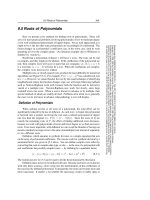
as a nonlinear function of displacement (u) given by
F
x
¼ ku
n

, which is shown graphically in Figure 7.1.
Here, k and n are some known constants. To determine
the work done by the force, a small strip of length du is
considered in the lower portion of the curve shown in
Figure 7.1. The work done by the force is obtained by
substituting the force variation in Equation (7.3) and
integrating, which is given by:
W ¼
ku
nþ1
n þ 1
¼
F
x
u
n þ 1
ð7:4Þ
Figure 7.1 Definitions of work (‘area OAB’) and complimen-
tary work (‘area OBC’).
Introduction to the Finite Element Method 147
Alternatively, work can also be defined as:
W

¼
ð
F
2
F
1
^

u  d
^
F ð7:5Þ
where, F
1
and F
2
are the initial and final applied forces.
The above definition is normally referred to as Comple-
mentary Work. Again, by considering a 1-D system with
the same nonlinear force–displacement relationship
(F
x
¼ ku
n
), we can write the displacement u as u ¼
ð1=kÞF
ð1=nÞ
x
. Substituting this into Equation (7.5) and
integrating, the complementary work can be written as:
W

¼
F
ð1=nþ1Þ
x
kð1=n þ 1Þ
¼
F

x
u
ð1=n þ 1Þ
ð7:6Þ
Obviously, W and W
*
are not the same although they
were obtained from the same curve. However, for the
linear case (n ¼ 1), they have the same value, given by
W ¼ W

¼ F
x
u=2, which is nothing but the area under
the force–displacement curve. The definition of Work is
normally used in the stiffness formulation, while the
concept of Complementary Work is normally used in
the force method of analysis.
7.2.2 Strain energy, complimentary strain energy
and kinetic energy
Consider an elastic body subjected to a set of forces and
moments. The deformation process is governed by the
First Law of Thermodynamics, which states that the total
change in the energy (ÁE) due to the deformation
process is equal to the sum of the total work done by
the elastic and inertial forces (W
E
) and the work done
due to head absorption (W
H

), that is:
ÁE ¼ W
E
þ W
H
If the thermal process is adiabatic, then W
H
¼ 0. The
energies associated with the elastic and the inertial forces
are called the Strain Energy (U) and Kinetic Energy (T),
respectively. If the loads are gradually applied, the time-
dependency of the load can be ignored, which essentially
means that the kinetic energy T can be assumed to be
equal to zero. Hence, the change in the energy ÁE ¼ U.
That is, the mechanical work done in deforming the
structure is equal to the change in the internal energy
(strain energy). When the structure behaves linearly and
the load is removed, the strain energy is converted back
to mechanical work.
To derive the expression for the strain energy, consider
a small element of volume dV of the structure under a
1-D state of stress, as shown in Figure 7.2. Let s
xx
be the
stress on the left face and s
xx
þð@s
xx
=@xÞdx be the stress
on the right face. Let B

x
be the body force per unit volume
along the x-direction. The strain energy increment dU due
to the stresses s
xx
on face 1 and s
xx
þð@s
xx
=@xÞdx on
face 2 during infinitesimal deformation du on face 1 and
dðu þð@u=@xÞdxÞ on face 2 is given by:
dU ¼s
xx
dydzdu þ s
xx
þ
@s
xx
@x
dx

dydzd u þ
@u
@x
dx

þ B
x
dydxdz

Simplifying and neglecting the higher-order terms, we
get:
dU ¼ s
xx
d
@u
@x

dxdydz þdudxdydz
@s
xx
@x
þ B
x

The last term within the brackets is the equilibrium
equation, which is equal to zero. Hence, the incremental
strain energy now becomes:
dU ¼ s
xx
d
@u
@x

dxdydz ¼ s
xx
de
xx
dV ð7:7Þ
Now, we introduce the term called incremental Strain

Energy Density, which we define as:
dS
D
¼ s
xx
de
xx
Integrating the above expression over a finite strain, we
get:
S
D
¼
ð
e
xx
0
s
xx
de
xx
ð7:8Þ
dx
dz
dy
xx
xx
xx
dx
x
Figure 7.2 Elemental volume for computing the strain energy.

148 Smart Material Systems and MEMS
Using the above expression in Equation (7.7) and inte-
grating it over the volume, we get
U ¼
ð
V
S
D
dV ð7:9Þ
Similar to the definition of work and complementary
work, we can define complimentary strain energy density
and complimentary strain energy as:
U

¼
ð
V
S

D
dV; S

D
¼
ð
s
xx
0
e
xx

ds
xx
ð7:10Þ
We can represent this graphically in a similar manner as
we did for work and complimentary work. This is shown
in Figure 7.3.
In this figure, the area of the region below the curve
represents the strain energy while the region above
the curve represents the complementary strain energy.
Since the scope of this chapter is limited to the Finite
Element Method, all of the theorems dealing with com-
plimentary strain energy will not be dealt with here.
Kinetic energy should also be considered in evaluating
the total energy if the inertial forces are important.
Inertial forces are predominant in time-dependent pro-
blems, where both loading and deformation have time
histories. Kinetic energy is given by the product of mass
and the square of velocity. This can be mathematically
represented in the integral form as:
T ¼
1
2
ð
V
rð
_
u
2
þ
_

v
2
þ
_
w
2
ÞdV ð7:11Þ
Here, u, v and w are the displacement in the three co-
ordinate directions while the dots on the characters
represent the first time derivatives and in this case are
the three respective velocities.
7.2.3 Weighted residual technique
Any system is governed by a differential equation of the
form:
Lu ¼ f ð7:12Þ
where L is the differential operator of the governing
equation, u is the dependent variable of the governing
equation and f is the forcing function.
The system may have two different boundaries t
1
and
t
2
, where the displacements u ¼ u
0
and tractions t ¼ t
0
,
respectively, are specified. The WRT is one of the ways
to construct many approximate methods of analysis. In

most approximate methods, we seek an approximate
solution for the dependent variable u by, say
"
u (in one
dimension), as:
"
uðx; tÞ¼
X
N
n¼1
a
n
ðtÞf
n
ðxÞð7:13Þ
Here, a
n
are some unknown constants, which are time-
dependent in dynamic situations, and f
n
are some known
functions, which are spatially dependent. When we use
discritization in the solution process as in the case of the
FEM, a
n
will represent the nodal coefficients. In general,
these functions satisfy the kinematic boundary conditions
of the problem. When Equation (7.13) is substituted
into the governing equation, we get L
"

u  f 6¼ 0 since the
assumed solution is approximate. We can define the error
function associated with the solution as:
e
1
¼ L
"
u  f ; e
2
¼
"
u  u
0
; e
3
¼
"
t t
0
ð7:14Þ
The objective of any weighted residual technique is to
make the error function as small as possible over the
domain of interest and also on the boundary. This can be
done by distributing the errors in different methods with
each method producing a new approximate method of
solution.
Let us consider a case where the boundary conditions
are exactly satisified, that is, e
2
 e

3
 0. In this case, we
need to distribute the error function e
1
only. This can
be done through a weighting function w and integrating
over the domain as:
ð
V
e
1
wdV ¼
ð
V
ðL
"
u  f ÞwdV ¼ 0 ð7:15Þ
Figure 7.3 Concepts of strain energy (‘area OAB’) and com-
plimentary strain energy (‘area OBC’).
Introduction to the Finite Element Method 149
Choice of the weighting functions determines the type
of WRT. The weighting functions used are normally of
the form:
w ¼
X
N
n¼1
b
n
c

n
ð7:16Þ
When Equation (7.16) is substituted into Equation (7.15),
we get:
X
N
n¼1
b
n
ð
V
ðL
"
u  f Þc
n
¼ 0; n ¼ 1; 2; 3; ; n
Since b
n
are arbitrary, we have:
ð
V
ðL"u f Þc
n
¼ 0; n ¼ 1; 2; ; n
This process ensures that the number of algebraic equa-
tions resulting in using Equation (7.13) for
"
u is equal to
the number of unknown coefficients chosen.
Now, we can choose different weighting functions to

obtain different approximate techniques. For example, if
we choose all of c
n
as the Dirac delta function, normally
represented by the d symbol, we get the classical finite
difference technique. These are the spike functions that
have a unit value only at the point that they are defined
while at all other points they are zero. They have the
following properties:
ð
1
1
dðx x
n
Þdx ¼
ð
xþr
xr
dðx x
n
Þdx ¼ 1
ð
1
1
f ðxÞdðx x
n
Þdx ¼
ð
xþr
xr

f ðxÞdðx x
n
Þdx ¼ f ðx
n
Þ
Here, r is any positive number and f(x) is any func-
tion that is continuous at x ¼ n. To demonstrate this
method, consider a three-point line element, as shown in
Figure 7.4.
The displacement field can be expressed as a three-
term series in Equation (7.13) as:
"
u ¼ u
n1
f
1
þ u
n
f
2
þ u
nþ1
f
3
ð7:17Þ
Here, the functions f
1
, f
2
and f

3
satisfy the boundary
conditions at the nodes, namely its nodal displacements,
and they are given by:
f
1
¼ 1 
x
L

1 
2x
L

; f
2
¼
4x
L

4x
2
L
2

;
f
3
¼
x

L
2x
L
 1

ð7:18Þ
Now the weighting function can be assumed as:
w ¼ b
1
dðx 0Þþb
2
dðx L=2Þþb
3
dðx LÞ
¼
X
3
n¼1
b
n
d
n
ð7:19Þ
Let us now try to solve the following simple 1-D ordinary
differential equation given by:
d
2
u
dx
2

þ 4u þ4x ¼ 0; uð0Þ¼uð1Þ¼0 ð7:20Þ
Here, the independent variable x has limits between 0 and
1. Using Equation (7.17) in Equation (7.20), one can find
the error function or residue e
1
, say at node n, given by:
e
1
¼
d
2
u
dx
2
þ 4u þ4x

n
¼
1
L
2
u
n1

2
L
2
u
n
þ

1
L
2
u
nþ1

þ 4u
n
þ 4x
n
ð7:21Þ
Here, L ¼ 1 is the domain length. If we now substitute
the weight function (Equation (7.19)) and integrate, and
using the properties of the Dirac delta function, we get:
1
L
2
ðu
n1
 2u
n
þ u
nþ1
Þ

þ 4u
n
þ 4x
n
¼ 0 ð7:22Þ

The above equation is the equation for the central finite
differences.
The method of moments can be derived by assuming
the weight functions of the form given by (for the 1-D
case):
w ¼ b
1
þ b
2
x þb
3
x
2
þ b
4
x
3
þ ¼
X
N
n¼0
b
n
x
n
ð7:23Þ
x = 0 x = L/2 x = L
n – 1 nn + 1
Figure 7.4 Finite differences, according to the weighted
residual technique (WRT).

150 Smart Material Systems and MEMS
Consider again the problem given in Equation (7.20). Let
us assume only the first two terms in the above series.
Let the field variable u be assumed as:
"u ¼ a
1
xð1 xÞþa
2
x
2
ð1  xÞð7:24Þ
Each of the functions associated with the unknown
coefficients satisfy the boundary conditions specified in
Equation (7.20). Substituting the above into the govern-
ing equation, the following residue is obtained:
e
1
¼ a
1
ð2 þ4x 4x
2
Þþa
2
ð2  6x þ4x
2
 4x
3
Þþ4x
ð7:25Þ
If we weight this residual, we get the following

equations:
ð
1
0
1e
1
dx ¼ 2a
1
þ a
2
¼ 3;
ð
1
0
xe
1
dx ¼ 5a
1
þ 6a
2
¼ 10
Solving the above two equations, we get a
1
¼ 8=7 and
a
2
¼ 5=7. Substituting these, we get the approximate
solution to the problem as:
"
u ¼

8
7
xð1 xÞþ
5
7
x
2
ð1  xÞ
The exact solution to Equation (7.20) is given by:
u
exact
¼
sin ð2xÞ
sin ð2Þ
 x
To compare the results, say at x ¼ 0:2, we get "u ¼ 0:205
and u
exact
¼ 0:228. The percentage error involved in the
solution is about 10, which is very good considering that
only two terms were used in the weight-function series.
Next, the procedure of deriving the Galerkin technique
from the weighted residual method is outlined.
Here, we assume the weight-function variation to be
similar to the displacement variation (Equation (7.13)),
that is:
w ¼ b
1
f
1

þ b
2
f
2
þ b
3
f
3
þ : ð7:26Þ
Let us now consider the same problem (Equation (7.20))
with the assumed displacement field given by
Equation (7.24). Let the weight function variation have
only the first two terms in the series, as:
w ¼ b
1
f
1
þ b
2
f
2
¼ b
1
xð1 xÞþb
2
x
2
ð1  xÞð7:27Þ
The residual e
1

is the same as that given for the previous
case (Equation (7.25)). If we weight this residual with the
weight function given by Equation (7.27), the following
equations are obtained:
ð
1
0
f
1
e
1
dx ¼ 6a
1
þ 3a
2
¼ 10;
ð
1
0
f
2
e
1
dx ¼ 21a
1
þ 20a
2
¼ 42
Solving the above equations, we get a
1

¼ 74=57 and
a
2
¼ 42=57. The approximate Galerkin solution then
becomes:
"
u ¼
74
57
xð1 xÞþ
42
57
x
2
ð1 xÞ
The result obtained for x ¼ 0:2 is 0.231, which is very
close to the exact solution (only a 1.3 % error).
In a similar manner, one can design various approxi-
mate schemes by assuming different weight functions.
The FEM is one such WRT, wherein the displacement
variation and the weight functions are the same. The
‘weak form’ of the differential equation becomes the
equation involving the energies.
7.3 ENERGY FUNCTIONALS
AND VARIATIONAL OPERATOR
The use of the energy functional is an absolute necessity
for development of the finite element method. The energy
functional is essentially dependent on a number of depen-
dent variables, such as displacements, forces, etc. which
themselves are functions of position, time, etc. Hence, a

functional is an integral expression, which in essence is
the ‘function of many functions’. A formal study in the
area of energy functionals requires a deep understanding
of functional analysis. Reddy [3] gives an excellent
account of the FEM from the functional analysis view-
point. However, we, for the sake of completeness, merely
state those important aspects that are relevant for finite
element development. These are mathematically repre-
sented between the limits a and b as:
IðwÞ¼
ð
b
a
Fx; w;
dw
dx
;
d
2
w
dx
2

ð7:28Þ
Introduction to the Finite Element Method 151
Here, a and b are the two boundary points in the domain.
For a fixed value of w, I(w) is always a scalar. Hence, a
functional can be thought of as a mapping of I(w) from
a vector space W to a real number field R, which is
mathematically represented as I : W ! R. A functional

is said to be linear if it satisfies the following condition:
Fðaw þbvÞ¼aFðwÞþbFðvÞð7:29Þ
Here, a and b are some scalars and w and v are the depen-
dent variables.
A functional is called quadratic functional, when the
following relation exist:
Iða wÞ¼a
2
IðwÞð7:30Þ
If there are two functions p and q, their inner product
over the domain V can be defined as:
ðp; qÞ¼
ð
V
pqdV ð7:31Þ
Obviously, the inner product can also be thought of as a
functional. We can use the above definition to determine
the properties of the differential operator of a given dif-
ferential equation. A given problem is always defined by
a differential equation and a set of boundary conditions,
which can be mathematically represented by:
Lu ¼ f ; over the domain V
u ¼ u
0
; over t
q ¼ q
0
; over t
2
ð7:32Þ

where L is the differential operator, V is the
entire domain, t
1
is the domain where the displacements
are specified (kinematic or essential boundary condi-
tions) and t
2
is the domain where the forces (natural
boundary conditions) are specified. If u
0
is zero, then we
call the essential boundary conditions homogenous.For
non-zero u
0
, the essential boundary condition becomes
non-homogenous. There is always a functional for a
given differential equation provided that the differential
operator L satisfies the following conditions:
 The differential operator L requires to be self-adjoint
or symmetric. That is, ðLu; vÞ¼ðu; LvÞ, where u and v
are any two functions that satisfy the same appropriate
boundary conditions.
 The differential operator L requires to be positive
definite. That is, ðLu; uÞ0 for functions u satisfying
the appropriate boundary conditions. The equality
will hold only when u ¼ 0 everywhere in the domain.
The derivation of these relations is beyond the scope of
study here. The interested reader is advised to refer
to Shames and Dym [1] and Wazhizu [4] which are
classic textbooks on variational principles for elasticity

problems.
For a given differential equation, Lu ¼ f , that is,
subjected to homogenous boundary conditions with the
differential operator being self-adjoint and positive defi-
nite, one can actually construct the functional. This is
given by the following expression:
IðwÞ¼ðLw; wÞ2ðw; f Þð7:33Þ
To see what the above equation means, let us construct
the functional for the well-known beam governing
equation, which is given by:
EI
d
4
w
dx
4
þ q ¼ 0
In the above equation, EI is the bending rigidity, w is
the dependent variable, which represents the transverse
displacements, x is the independent spatial variable
and q represents the loading. The domain is represented
by the length of the beam l. In the above equation,
L ¼ EId
4
=dx
4
and f ¼q.Now,thefirst term in
Equation (7.33) becomes:
ðLw; wÞ¼
ð

l
0
EI
d
4
w
dx
4
wdx
Integrating by parts, we get:
ðLw; wÞ¼wEI
d
3
w
dx
3

x¼l
x¼0

ð
l
0
EI
d
3
w
dx
3
dw

dx
dx
The first term is the boundary term which has two
parts – one is the displacement boundary condition
while the second part (EId
3
w=dx
3
) is the force boundary
condition and in the present case, represents the shear
force. For a right-hand coordinate system, this is denoted
by V. Hence, the above equation can be written as:
ðLw; wÞ¼wð0ÞVð0ÞþwðlÞVðlÞ
ð
l
0
EI
d
3
w
dx
3
dw
dx
dx
152 Smart Material Systems and MEMS
Integrating again the last part of the above equation by
parts, we get:
ðLw; wÞ¼wð0ÞVð0ÞþwðlÞVðlÞ
dw

dx
EI
d
2
w
dx
2

x¼l
x¼0
þ
ð
l
0
EI
d
2
w
dx
2
d
2
w
dx
2
dx
¼wð0ÞVð0ÞþwðlÞVðlÞfðlÞMðlÞ
þ fð0ÞMð0Þþ
ð
l

0
EI
d
2
w
dx
2

2
dx ð7:34Þ
Here, f is the rotation of the cross-section (also called
the slope) and M is the moment resultant. There are three
possible boundary conditions in the beam, namely:
 Fixed end condition, where w ¼
dw
dx
¼ f ¼ 0.
 Free boundary condition, where V ¼EI
d
3
w
dx
3
¼
M ¼ EI
d
2
w
dx
2

¼ 0.
 Hinged boundary condition, where w ¼ M ¼ EI
d
2
w
dx
2
¼ 0.
For all of these boundary conditions, the boundary terms in
Equation (7.34) are zero and hence the equation reduces to:
ðLw; wÞ¼2
1
2

ð
l
0
EI
d
2
w
dx
2

2
dx ð7:35Þ
Substituting the above into Equation (7.33), we can write
the functional as:
IðwÞ¼2
1

2
ð
l
0
EI
d
2
w
dx
2

2
dx þ
ð
l
0
qwdx
2
4
3
5
ð7:36Þ
The terms inside the bracket are the total potential energy
of the beam and the value of the functional is essentially
twice the value of the potential energy. Hence, the func-
tionals in structural mechanics are normally called
energy functionals. We see from the above derivations
that the boundary conditions are contained in the energy
functional.
7.3.1 Variational symbol

In most approximate methods based on variational
theorems, including the finite element technique, it is
necessary to minimize the functional and this mini-
mization process is normally represented by a varia-
tional symbol (normally referred to as delta operator),
mathematically represented as d. Consider a functional
that is a function of the dependent-variable w and
its derivatives and is mathematically represented as
Fðw; w
0
; w
00
Þ,wheretheprimesð
0
Þ and ð
00
Þ indicate the
first and second derivatives, respectively. For a fixed
value of the independent variable x, the value of the
functional depend on w and its derivatives. During the
process of deformation, if the value of w changes to au,
where a is a constant and u is a function, then this
change is called the variation of w and is denoted by
dw.Thatis,dw represents the admissible change of w
for a fixed value of the independent variable x.Atthe
boundary points, where the values of the dependent
variables are specified, the variations at these points
are zero. In essence, the variational operator acts like
a differential operator and hence all of the laws of
differentiation are applicable here.

7.4 WEAK FORM OF THE GOVERNING
DIFFERENTIAL EQUATION
The variational method gives us an alternate statement
of the governing equation, which is normally referred
to as the strong form of the governing equation. This
alternate statement of the equilibrium equation is essen-
tially an integral equation. This is essentially obtained
by weighting the residue of the governing equation
with a weighting function and integrating the resulting
expression. This process not only gives the weak
form of the governing equation, but also the associated
boundary conditions (both essential and natural bound-
ary conditions). We will explain this procedure by
again considering the governing equation of an elemen-
tary beam. The ‘strong’ form of the beam equation is
given by:
EI
d
4
w
dx
4
þ q ¼ 0
Now, we are looking for an approximate solution for
"
w
in a similar form to that given in Equation (7.13). Now,
the residue becomes:
EI
d

4
"
w
dx
4
þ q ¼ e
1
Introduction to the Finite Element Method 153
If we weight this with another function v (which also
satisfies the boundary conditions of the problem) and
integrate over the domain of length l, we get:
ð
l
0
EI
d
4
"
w
dx
4
þ q

vdx
Integrating the above expression by parts (twice), we will
get the boundary terms, which are a combination of both
essential and natural boundary conditions, along with
the weak form of the equation. We obtain the following
expression:
vð0Þ

"
Vð0ÞvðlÞ
"
VðlÞfðlÞ
"
MðlÞþfð0Þ
"
Mð0Þ
þ
ð
l
0
EI
d
2
"
w
dx
2
d
2
v
dx
2
þ qv

dx ð7:37Þ
where
"
V ¼EId

3
"w=dx
3
;
"
M ¼EId
2
"w=dx
2
and f¼d"w=dx.
Equation (7.37) is the weak form of the differential
equation as it requires a reduced continuity requirement
when compared to the original differential equation.
That is, the original equation is a fourth-order equation
and requires functions that are third-order continuous,
while the weak order requires solutions that are just
second-order continuous. This aspect is exploited fully
in the finite element method.
7.5 SOME BASIC ENERGY THEOREMS
In this section, we outline three different theorems, which
essentially form the backbone of finite element analysis.
Here, the implications of these theorems on the develop-
ment of finite element techniques are discussed. For a
more thorough discussion on these topics, the interested
reader is advised to refer to some classic textbooks
available in this area, such as Shames and Dym [1],
Wazhizu [4] and Tauchert [5]. Here, we discuss the fol-
lowing important energy principles:
 Principle of Virtual Work (PVW).
 Principle of Minimum Potential Energy (PMPE).

 Rayleigh–Ritz method.
 Hamilton’s principle (HP).
While the first two are essential for FE development for
static problems, the last theorem is used for deriving the
weak form of the equation for time-dependent problems.
This section will also describe a few approximate meth-
ods which are ‘offshoots’ of these theorems.
7.5.1 Concept of virtual work
Consider a body shown in Figure 7.5, under the action of
an arbitrary set of loads P
1
, P
2
, etc. In addition, consider
any arbitrary point which is subjected to a kinemati-
cally admissible infinitesimal deformation. By ‘kinema-
tically admissible’, we mean that it does not violate the
boundary constraints. Work done by such small hypothe-
tical infinitesimal displacements, due to applied loads
which are kept constant during the deformation process,
is called virtual work. We denote the virtual displacement
by the variational operator d and in this present case it
can be written as du.
7.5.2 Principle of virtual work (PVW)
This principle states that a continuous body is in equili-
brium, if and only if, the virtual work done by all of the
external forces is equal to the virtual work done by
internal forces when the body is subjected to a infinite-
simal virtual displacement.IfW
E

is the work done by the
external forces and U is the internal energy (also called
the strain energy), then the PVW can be mathematically
represented as:
dW
E
¼ dU ð7:38Þ
Proof
Let us consider a three-dimensional body of ‘arbitrary
material behavior’ which is subjected to surface traction
t
i
on a portion of the body of area S and a body force per
unit volume B
i
. The total external work done by the body
of volume V on displacements u
i
is given by:
W
E
¼
ð
S
t
i
u
i
dS þ
ð

V
B
i
u
i
ð7:39Þ
By taking variation of this work, we get:
dW
E
¼
ð
S
t
i
du
i
dS þ
ð
V
B
i
du
i
ð7:40Þ
u
Figure 7.5 Representation of a body under virtual displace-
ments.
154 Smart Material Systems and MEMS
Substituting for ‘tractions’ from Equation (6.33) in
Chapter 6 in the above equation, we get:

dW
E
¼
ð
S
s
ij
n
i
du
i
dS þ
ð
V
B
i
du
i
ð7:41Þ
Here, n
i
is the surface normal of the body where the
‘tractions’ are acting. The surface integral on the right-
hand side of the above equation is converted to a volume
integral by using the divergence theorem [1] which
states:
ð
V
rudV ¼
ð

S
undS ð7:42Þ
where r¼ð@=@xÞi þð@=@yÞj þð@=@zÞk is the gradient
operator, u ¼ðui þvj þ wzÞ is the displacement vector
and n ¼ðn
x
i þn
y
j þn
z
kÞ is the outward normal vector.
Using Equation (7.42) in Equation (7.41) and simplify-
ing, we get:
dW
E
¼
ð
V
s
ij
@
@x
j
ðdu
i
Þ
|fflfflfflfflffl{zfflfflfflfflffl}
Virtual strain
dV þ
ð

V
@
@x
j
ðs
ij
Þdu
i
dV þ
ð
V
B
i
du
i
¼
ð
V
s
ij
de
ij
dV
|fflfflfflfflffl{zfflfflfflfflffl}
Internal virtual work¼dU
þ
ð
V
@
@x

j
ðs
ij
ÞþB
i

du
i
dV
|fflfflfflfflfflfflfflfflfflfflfflfflfflfflfflfflfflfflffl{zfflfflfflfflfflfflfflfflfflfflfflfflfflfflfflfflfflfflffl}
Equation of equilibrium¼0
Further simplifying, the external virtual work becomes
dW
E
¼ dU, which is essentially the virtual work principle.
The direct offshoot of PVE is the Dummy Displace-
ment method, which is extensively used for finding
the reaction forces in many redundant structures. The
details of this method can be found in Tauchert [5] and
Reddy [6].
7.5.3 Principle of minimum potential energy
(PMPE)
This principle states that of all the displacement fields
which satisfy the prescribed constraint conditions, the
correct state is that which makes the total potential
energy of the structure a minimum.
This principle can be directly obtained from the PVW.
Here, we define the potential of the external forces V as
the negative of the work done by the external forces. That
is, V ¼W

E
. Using this in the PVW expression, we have:
dðU þ VÞ¼0 ð7:43Þ
The above principle is the backbone for finite element
development. In addition, this principle can be used to
derive the governing differential equations of the system,
especially for static analysis, and also their associated
boundary conditions. This aspect is demonstrated here by
deriving the governing equation for a beam, starting from
the energy functional.
Consider a beam of bending rigidity EI and subjected to
a distributed loading of qðxÞ per unit length over the entire
beam of length L.LetwðxÞ represent the lateral displace-
ment field of the beam. The strain energy functional and
the potential of the external forces can be written as:
U ¼
1
2
ð
L
0
EI
d
2
w
dx
2

2
dx; V ¼

ð
L
0
qwdx ð7:44Þ
By the PMPE, we have:
d
1
2
ð
L
0
EI
d
2
w
dx
2

2
dx 
ð
L
0
qwdx
2
4
3
5
¼ 0
Using the operation on the variational operator, we have:

ð
L
0
EI
d
2
w
dx
2

d
d
2
w
dx
2

dx 
ð
L
0
qdwdx
2
4
3
5
¼ 0
¼
ð
L

0
EI
d
2
w
dx
2

d
2
ðdwÞ
dx
2

dx 
ð
L
0
qdwdx
2
4
3
5
¼ 0
Integrating the first term by parts (twice) and identifying
the boundary terms, as was carried out earlier, we get:
dwð0ÞVð0ÞdwðLÞVðLÞdfðLÞMðLÞdfð0ÞMð0Þ
þ
ð
L

0
EI
d
4
w
dx
4
þ q

dwdx ¼ 0
Since the variation of the displacements at the specified
locations (boundaries) is always zero and dw is arbitrary,
the only non-zero term contained in the large bracket
should be the governing differential equation of the beam.
The PMPE can be directly used to derive the well-
known Castigliano’s first theorem used in elementary
structural mechanics to determine the reaction forces in
a structure discritized by using n generalized degrees
of freedom, q
n
. Both the strain energy, as well as the
potential of external forces, are functions of these
Introduction to the Finite Element Method 155
generalized degrees of freedom. Hence, we can write
the PMPE statement as:
d Uðq
n
Þ
X
N

n¼1
P
n
q
n
"#
¼ 0
Here, P
n
represent the applied load. Taking the first vari-
ation of the strain energy and expanding, we can write
the above expression as:
@U
@q
1
dq
1
þ
@U
@q
2
dq
2
þ þ
@U
@q
n
dq
n
 P

1
dq
1
 P
2
dq
2
  P
n
dq
n
¼ 0
Grouping the terms together, we have:
@U
@q
1
 P
1

dq
1
þ
@U
@q
2
 P
1

dq
1

þ
þ
@U
@q
n
 P
n

dq
n
¼ 0
Since all of the dq
n
are arbitrary, the terms contained in
each bracket should be equal to zero. Hence, we have:
@U
@q
n
 P
n

¼ 0; or
@U
@q
n
¼ P
n
ð7:45Þ
The above statement is essentially the Castigliano’s
theorem, which states that, if a reaction force at a gene-

ralized degree of freedom is required, then differentiating
the strain energy with respect to the said degree of
freedom will give the required reaction force.
The PMPE can also be used to construct some approxi-
mate solutions to the problem, One such method is the
Rayleigh–Ritz method [1]. This is one of the most import-
ant methods in structural mechanics for determining
an approximate solution to a problem. In fact, the Finite
Element Method can be considered as a ‘piecewise’
Rayleigh–Ritz method, where this technique is applied
at the element level and the total solution is obtained by
synthesis of element level solutions. This method is
explained next.
7.5.4 Rayleigh–Ritz method
In this method, we are seeking an approximate solution
to the governing equation Lu ¼ f , where u is the depen-
dent variable normally representing displacements in
structural mechanics. We again assume the approximate
solution in the form:
"
u ¼
X
N
n¼1
a
n
f
n
ð7:46Þ
Here, a

n
are the unknown generalized degrees of freedom
and f
n
are the known functions – called the Ritz func-
tions. These functions should satisfy the kinematic bound-
ary conditions and need not satisfy the natural boundary
conditions. Next, the strain energy and the potential of
external forces are written in terms of displacements and
the assumed approximate displacement field (Equation
(7.46)) and are substituted into the energy expressions
and integrated. The PMPE is invoked and the total energy
is minimized to get a set of n simultaneous equation,
which are solved for determining a
n
. Mathematically, we
can represent the total energy, which is function of a
n
,as:
pða
n
Þ¼ðU þ VÞ
By the PMPE, we have that the first variation of the total
energy is zero. That is:
dp ¼ 0 ¼
@p
@a
1
da
1

þ
@p
@a
2
da
2
þ þ
@p
@a
n
da
n
¼
X
N
n¼1
@p
@a
n
da
n
Since da
n
is arbitrary, we have:
@p
@a
1
¼
@p
@a

2
¼ : ¼
@p
@a
n
¼ 0; n ¼ 1; 2; n
This procedure ensures that there are n equations to solve
n unknown coefficients. The Ritz functions should be so
chosen that they be differentiable up to the order specified
by the energy functional. Normally polynomials or trigo-
nometric functions are used as Ritz functions. Since the
natural boundary conditions are not satisfied by the
assumed field, it is highly likely that the solutions would
not yield accurate forces (stresses). Normally, enough
terms should be used in Equation (7.46) to get accurate
solutions. However, if very few terms are used, then
these introduce additional geometric constraints which
make the structure stiffer and hence the predicted displa-
cements are always ‘lower-bound’. The application of this
method to problems of complex geometry is very difficult.
7.5.5 Hamilton’s principle (HP)
This principle is extensively used to derive the govern-
ing equation of motion for a structural system under
156 Smart Material Systems and MEMS
dynamic loads. In fact, this principle can be thought of
as the PMPE for a dynamic system. This principle was
first formulated by an Irish mathematician and physi-
cist, Sir William Hamilton. Similar to the PMPE, the HP
is an integral statement of a dynamic system under
equilibrium.

In order to derive this principle, consider a body of
mass m and having a position vector with respect to its
coordinate system as r ¼ xi þyj þzk. Under the action
of a force FðtÞ¼F
x
ðtÞi þF
y
ðtÞj þF
z
ðtÞk, this mass
moves from position 1 at time t
1
to a position 2 at
time t
2
, according to Newton’s Second Law. Such a
path is called the Newtonian Path. The motion of this
mass is pictorially shown in Figure 7.6.
The total force FðtÞ comprises conservative forces such
as internal forces caused by the strain energies of the
structures, the external forces and some non-conservative
forces, such as damping forces. Hence the force vector is
made up of two parts, which can be written as
FðtÞ¼F
c
ðtÞþF
nc
ðtÞ. Each of these will have compo-
nents in all of the three coordinate directions. This force
is balanced by the inertial force generated by the moving

mass. If this mass is given a small virtual displacement,
drðtÞ¼dui þ dvj þdwk, where u, v and w are the dis-
placement components in the three coordinate direc-
tions, the path of mass is as shown by the dashed line in
Figure 7.6. This path need not be a ‘Newtonian path’,
however, at time t ¼ t
1
and t ¼ t
2
, the path coincides
with the ‘Newtonian path’ of the original motion of the
mass. That is, we have drðt
1
Þ¼drðt
2
Þ¼0. The equili-
brium of this mass can be written as:
F
x
ðtÞm
€
uðtÞ¼0;
F
y
ðtÞm
€
vðtÞ¼0;
F
z
ðtÞm

€
wðtÞ¼0
Invoking the PVM, which essentially states that the total
virtual work done by the infinitesimal virtual displace-
ment should be zero, we have:
½F
x
ðtÞm
€
uðtÞduðtÞþ½F
y
ðtÞm
€
vðtÞdvðtÞ
þ½F
z
ðtÞm
€
wðtÞdwð tÞ¼0 ð7:47Þ
Rearranging the terms and integrating the equation
between the time t
1
and time t
2
, we have:
ð
t
2
t
1

m½€uðtÞduðtÞþ€vðtÞdvðtÞþ€wðtÞdwðtÞ
þ
ð
t
2
t
1
½F
x
ðtÞduðtÞþF
y
ðtÞdvðtÞþF
z
ðtÞdwðtÞ ð7:48Þ
Consider the first integral (I
1
), which can be written after
integrating by parts as:
I
1
¼m
_
uðtÞduðtÞm
_
vðtÞdvðtÞm
_
wðtÞdwðtÞ
t¼t
2
t¼t

1
þ
ð
t
2
t
1
mð_ud_u þ _vd_v þ _wd _wÞdt
Recognizing that the virtual displacement must vanish at
the beginning and end of this varied path, we can write
the first integral as:
I
1
¼
ð
t
2
t
1
mð
_
ud
_
u þ
_
vd
_
v þ
_
wd

_
wÞdt
¼
ð
t
2
t
1
m
2
dð_u
2
þ _v
2
þ _w
2
Þdt ¼ d
ð
t
2
t
1
Tdt ð7:49Þ
Here, T represents the total kinetic energy of the sys-
tem. Now, let us consider the second integral (I
2
)in
Equation (7.48). The force term in this expression can be
written in terms of internal and non-conservative forces.
This integral then becomes:

I
2
¼
ð
t
2
t
1
½F
cx
ðtÞduðtÞþF
cy
ðtÞdvðtÞþF
cz
ðtÞdwðtÞdt
þ
ð
t
2
t
1
½F
ncx
ðtÞduðtÞþF
ncy
ðtÞdvðtÞþF
ncz
ðtÞdwðtÞdt
x
y

z
i
j
k
r
(t)
F(t)
mr(t)
r(t)
t
2
t
1
Real path
Variable
r(t) = xi + yj + zk
Figure 7.6 Real and variable paths for a particle of mass m.
Introduction to the Finite Element Method 157
The second integral in the above expression is nothing
but the variation of the work done by the non-conservative
forces and can be written as:
d
ð
t
2
t
1
W
nc
dt ¼ d

ð
t
2
t
1
½F
ncx
ðtÞuðtÞþF
ncy
ðtÞvðtÞ
þF
ncz
ðtÞwðtÞdt
The first integral in I
2
is the work done due to internal
forces. From Castigliano’s first theorem, which was
derived in Section 7.5.3, the internal force is obtained
by differentiating the strain energy ðUðu; v; w; tÞÞ with
respect to the corresponding displacement (Equation
(7.45)). Accordingly, we can write:
F
cx
¼
@U
@u
; F
cy
¼
@U

@v
; F
cz
¼
@U
@w
ð7:50Þ
The negative sign is given to indicate that these forces
resist the deformation. Using Equation (7.50) in I
2
,we
have:
I
2
¼
ð
t
2
t
1
@U
@u
duðtÞþ
@U
@v
dvðtÞþ
@U
@w
dwðtÞ


dt
þ d
ð
t
2
t
1
W
nc
dt
¼ d
ð
t
2
t
1
ðU þ W
nc
Þdt
ð7:51Þ
By using Equations (7.49) and (7.51) in Equation (7.48),
Hamilton’s principle becomes:
d
ð
t
2
t
1
ðT  U þ W
nc

Þdt ¼ 0 ð7:52Þ
The use of this equation in obtaining the governing equa-
tion and its associated boundary conditions was demon-
strated in Section 6.3.2 in the last chapter. It is of interest
to know that if we omit the inertial energy in Equation
(7.52) and assume that all of the quantities are time-
independent, then the HP reduces to the PMPE.
One can easily deduce the famous Lagrange Equa-
tion of motion for a discrete system having the energies
(kinetic, strain energy and non-conservative energy) as a
function of the generalized coordinates q
1
; q
2
; q
n
as:
T ¼ Tðq
1
; q
2
; q
n
;
_
q
1
;
_
q

2
;
_
q
n
Þ
U ¼ Uðq
1
; q
2
; q
n
Þ
W
nc
¼ P
1
q
1
þ P
2
q
2
þ P
n
q
n
ð7:53Þ
Here, P
1

; P
2
; P
n
represent the external and damping
forces. Taking the first variation of these energies, we
have:
dT ¼
@T
@q
1
dq
1
þ
@T
@q
2
dq
2
þ þ
@T
@q
n
dq
n
þ
@T
@
_
q

1
d
_
q
1
þ
@T
@ _q
2
d
_
q
2
þ þ
@T
@ _q
n
d
_
q
n
¼
X
n
i¼1
@T
@q
i
dq
i

þ
@T
@ _q
i
d
_
q
i
dU ¼
@U
@q
1
dq
1
þ
@U
@q
2
dq
2
þ þ
@U
@q
n
dq
n
¼
X
n
i¼1

@U
@q
i
dq
i
dW
nc
¼ P
1
dq
1
þP
2
dq
2
þ P
n
dq
n
¼
X
n
i¼1
P
i
dq
i
Using the above in the HP (Equation (7.52)), we have:
X
n

i¼1
ð
t
2
t
1
@T
@q
i
dq
i
þ
@T
@
_
q
i
d
_
q
i

@U
@q
i
dq
i
þ P
i
dq

i

dt ¼ 0
ð7:54Þ
Integrating the second term by parts and recognizing that
the virtual displacements vanish at the beginning and
end, the above integral becomes:
ð
t
2
t
1
X
n
i¼1

d
dt
@T
@
_
q
i

þ
@T
@q
i

@U

@q
i
þ P
i

dq
i
¼ 0
Since the virtual displacements are arbitrary, the
Lagrange equations become:
d
dt
@T
@
_
q
i


@T
@q
i
þ
@U
@q
i
¼ P
i
ð7:55Þ
The above equation is extensively used in the derivation

of discritized equations of motion for a dynamic system.
7.6 FINITE ELEMENT METHOD
The FEM uses the ‘weak form’ of the governing equation
to convert a ordinary differential equation to a set of
algebraic equations in the case of static analysis and a
158 Smart Material Systems and MEMS
coupled set of second-order differential equations in the
case of dynamic analysis. In the previous sections of this
chapter, different approximate methods were explained,
which are very difficult to apply to a problem involving
complex geometry and complicated boundary conditions.
However, if one takes the approach of subdividing the
domain into many subdomains, in each of these sub-
domains, one can assume a solution of the type:
"
uðx; y; z; tÞ¼
X
N
n¼1
a
n
ðtÞf
n
ðx; y; zÞð7:56Þ
and fit any of the approximate methods described earlier
within the subdomains to get an approximate solution to
the problem. In the FEM, these subdomains are called
elements, which normally take the shapes of line ele-
ments for 1-D structures, such as rods and beams,
rectangles or triangles for 2-D structures and bricks or

tetrahedrons for 3-D structures. Each element has a set of
nodes, which may vary depending on the order of the
functions f
n
ðx; y; zÞ in Equation (7.56) used to approxi-
mate the displacement fields within each element. These
nodes have unique IDs, which fix their positions in space
of complex structures. In Equation (7.56), a
n
ðtÞ normally
represents the time-dependent nodal displacements,
while f
n
ðx; y; zÞ are the spatially dependent functions,
which are normally referred to as shape functions. The
entire finite element procedure for obtaining a solution
for a complex problem can be summarized as follows:
 The use of the weak form of the governing differential
equation and an assumption of the field-variable vari-
ation over the element (Equation (7.56)) and its subse-
quent minimization will yield a stiffness matrix and a
mass matrix. The sizes of these matrices depend on
the number of nodes and the number of degrees of
freedom each node can support. The mass matrix
formulated through the weak form of the equation is
called the consistent mass matrix. There are other
ways of formulating the mass matrix, which are
explained in detail in the latter part of this chapter.
The damping matrix is normally not obtained through
weak formulation. For linear systems, this is obtained

through a linear combination of stiffness and the mass
matrix. Damping through such a procedure is called
proportional damping.
 The FEM comes under the category of the stiffness
method, where satisfaction of the compatibility is
automatic as we begin the analysis with a displace-
ment assumption. The issue in the stiffness method is
satisfaction of the equilibrium equations. This
condition requires to be enforced. Such an enforce-
ment is made by assembling the stiffness, mass and
damping matrices. This is done by adding the stiffness
of a particular degree of freedom coming from the
contiguous elements. Similarly, the force vectors act-
ing on each node are assembled to obtain the global
force vector. If the load is distributed on a segment of
the complex domain, then using the equivalent energy
concept, it is split into concentrated loads acting on
the respective nodes that make up the segment. The
size of the assembled stiffness, mass and damping
matrices is equal to n n, where n is the total number
degrees of freedom in the discritized domain.
 After assembly of the matrices, the displacement
boundary conditions are enforced, which could be
homogenous or non-homogenous. If the boundary
conditions are homogenous, then the corresponding
rows and columns are eliminated to get the reduced
stiffness, mass and damping matrices. In the case of
static analysis, the obtained matrix equation involving
the stiffness matrix is solved to obtain the nodal
displacements. In the case of dynamic analysis, we

get a coupled set of ordinary differential equations,
which are solved by either modal methods or a ‘time-
marching’ scheme.
7.6.1 Shape functions
The spatial dependent function in Equation (7.56) is
called the shape function of the element. These functions
are normally assumed as being polynomial, whose order
depends on the degrees of freedom that an element can
support. These functions relate the nodal displacements
with the assumed displacement field. They are normally
denoted by the symbol N. We will now give the proce-
dure of finding the shape functions for the elements
shown in Figure 7.7.
7.6.1.1 Rod element
Let us now derive the shape functions for a finite rod ele-
ment having length L and axial rigidity EA.A
rod element can support only axial motion and hence
this element can have two nodes and each node can
support one axial motion, as shown in Figure 7.7(a). That
is, we require a function that is only first order contin-
uous (that is C
0
continuous elements). Hence, we can
assume the displacement field contains two constants
corresponding to two degrees of freedom, that is:
u ¼ a
0
ðtÞþa
1
ðtÞx ð7:57Þ

Introduction to the Finite Element Method 159
The above equation also happens to satisfy the governing
static differential equation of a rod, which is given
by EAd
2
u=dx
2
¼ 0. Equation (7.57) is now converted in
terms of nodal coordinates by substituting uðx ¼ 0Þ¼u
1
and uðx ¼ LÞ¼u
2
in the above equation. This will enable
us to write constants a
0
and a
1
in terms of the nodal
displacements u
1
and u
2
. Eliminating these constants and
simplifying, Equation (7.57) can now be written as:
uðxÞ¼ 1 
x
L

u
1

þ
x
L

u
2
ð7:58Þ
In Equation (7.58), the two functions inside the brackets
are the two shape functions of the rod corresponding to
two degrees of freedom. Hence, the displacement field
can be written in matrix form as:
uðxÞ¼½N
1
ðxÞ N
2
ðxÞ
u
1
u
2

¼½Nfugð7:59Þ
The shape function N
1
takes the value of 1 at node one
while it is zero at node two. Similarly, N
2
is zero at node 1
and one at node 2. In fact, the displacement for any element
can be written in the form shown in Equation (7.59).

7.6.1.2 Beam element
One can similarly derive the shape functions for a beam
element. The beam element shown in Figure 7.7(b) has
two nodes and each node have two degrees of freedom,
namely the transverse displacement w and rotation
f ¼ðdw=dxÞ. Hence, the nodal degrees of freedom
vector is given by fug¼fw
1
f
1
w
2
f
2
g
T
, which
requires a minimum cubic polynomial for displacement.
In addition, since the slope is derived from the transverse
displacements, it is required that the polynomial is
second-order continuous, that is, it requires a higher
continuity when compared to the rod. Such elements
are called C
1
continuous elements. We proceed as fol-
lows to obtain the shape functions. The interpolating
polynomial for the beam is given by:
wðx; tÞ¼a
0
ðtÞþa

1
ðtÞx þ a
2
ðtÞx
2
þ a
3
ðtÞx
3
ð7:60Þ
As in the case of rods, the above solution happens to be
the exact solution to the governing beam equation. Now,
if we substitute wð0; tÞ¼w
1
ðtÞ; fð0; tÞ¼dwð0; tÞ=dx
¼ f
1
ðtÞ; wðL; tÞ¼w
2
ðtÞ and fðL; tÞ¼dwðL; tÞ=dx ¼
f
2
ðtÞ, we get:
w
1
f
1
w
2
f

2
8
>
>
<
>
>
:
9
>
>
=
>
>
;
¼
10 0 0
01 0 0
1 LL
2
L
3
012L 3L
2
2
6
6
4
3
7

7
5
a
0
a
1
a
2
a
3
8
>
>
<
>
>
:
9
>
>
=
>
>
;
¼fug¼½Gfag
Inverting the above matrix, we can write the unknown
coefficients as fag¼½G
1
fug. Substituting the values
of the coefficients in Equation (7.60), we get:

wðx; tÞ¼½N
1
ðxÞ N
2
ðxÞ N
3
ðxÞ N
4
ðxÞfuðtÞg;
N
1
ðxÞ¼1 3
x
L

2
þ2
x
L

3
; N
2
ðxÞ¼x 1 
x
L

2
N
3

ðxÞ¼3
x
L

2
2
x
L

3
; N
4
ðxÞ¼x
x
L

2

x
L


ð7:61Þ
The above shape function will take a unit value at the
nodes and zero everywhere else.
Before we proceed further, we will highlight the
necessary requirements an interpolating polynomial of
an element has to satisfy, especially from the convergence
point of view. These can be summarized as follows:
 The assumed solution should be able to capture the

rigid body motion. This can be made sure by retaining
a constant part in the assumed solution.
 The assumed solution must be able to attain the
constant strain rate as the mesh is refined. This can
be assured by retaining the linear part of the assumed
function in the interpolating polynomial.
Figure 7.7 Different finite elements: (a) rod element; (b) beam
element; (c) rectangular element; (d) triangular element.
160 Smart Material Systems and MEMS
 Most second-order systems require only C
0
continu-
ity, which are easily met in most FE formulations.
However, for higher-order systems such as Bernoulli–
Euler beams or elementary plates, one requires C
1
continuity, which are extremely difficult to satisfy,
especially for plate problems, where interelement
slope continuity is very difficult to comply with. In
such situations, one can use shear-deformable models,
that is, models that also include the effect of shear
deformations. In such models, slopes are not derived
from the displacements and are independently inter-
polated. This relaxes the C
1
continuity requirement.
However, when such elements are used in thin-beam or
plate models, where the effects of shear deformations are
negligible, the displacements predicted would be many
orders smaller than the correct displacements. Such

problems are called shear-locking problems, which are
addressed in detail in a latter part of this chapter.
 The order of an assumed interpolating polynomial is
dictated by the highest order of the derivative appear-
ing in the energy functional. That is, the assumed
polynomial should be at least one order higher than
that appearing in the energy functional.
 In 2-D formulation, especially for C
1
continuity prob-
lems, the polynomials are chosen based on Pascal’s
triangle [7].
7.6.1.3 Rectangular element
We will now determine the shape functions for two-
dimensional elements. Let us now consider a rectangular
finite element of length 2a and width 2b, as shown in
Figure 7.7(c). This element has four nodes and each node
can support two degrees of freedom, namely the two
displacements, u(x, y) and v(x, y) in the two coordinate
directions. Since there are four nodes, we can assume the
interpolating polynomial as:
uðx; yÞ¼a
0
þ a
1
x þa
2
y þa
3
xy

vðx; yÞ¼b
0
þ b
1
x þb
2
y þb
3
xy ð7:62Þ
The above function has a linear variation of displace-
ment in both the coordinate directions and hence it is
normally referred to as a bi-linear element. In the above
interpolating polynomial, we substitute uða; bÞ¼u
1
,
vða;bÞ¼v
1
, uða;bÞ¼u
2
, vða;bÞ¼v
2
, uða;bÞ¼u
3
,
vða;bÞ¼v
3
, uða;bÞ¼u
4
and vða;bÞ¼v
4

. These help
us to relate the nodal displacements to the unknown
coefficients as fug¼ ½Gfag. Inverting the above rela-
tion and substituting for the unknown coefficients in
Equation (7.62), we can write the displacement field
and the shape functions as:
uðx;yÞ¼½Nfug¼½N
1
ðx;yÞ N
2
ðx;yÞ N
3
ðx;yÞ N
4
ðx;yÞfug
vðx;yÞ¼½Nf vg¼½N
1
ðx;yÞ N
2
ðx;yÞ N
3
ðx;yÞ N
4
ðx;yÞfvg
fug¼fu
1
u
2
u
3

u
4
g
T
; fvg¼fv
1
v
2
v
3
v
4
g
T
N
1
ðx;yÞ¼
ðxaÞðybÞ
4ab
; N
2
ðx;yÞ¼
ðxaÞðyþbÞ
4ab
;
N
3
ðx;yÞ¼
ðxþaÞðyþbÞ
4ab

; N
4
ðx;yÞ¼
ðxþaÞðybÞ
4ab
ð7:63Þ
7.6.1.4 Triangular element
One can similarly write the shape functions for a triangle.
However, it is very convenient if one uses the area coordi-
nates for the triangle. Consider the triangle shown in
Figure 7.7(d), having coordinates of the three vertices as
ðx
1
; y
1
Þ, ðx
2
; y
2
Þ and ðx
3
; y
3
Þ.
Consider an arbitrary point P inside the triangle. This
point will split the triangle into three smaller triangles of
area A
1
, A
2

and A
3
, respectively. Let A be the total area of
the triangle, which can be written in terms of nodal
coordinates as
A ¼
1
2
1 x
1
y
1
1 x
2
y
2
1 x
3
y
3













ð7:64Þ
We will define the area coordinates for the triangle as:
L
1
¼
A
1
A
; L
2
¼
A
2
A
; L
3
¼
A
3
A
ð7:65Þ
Thus, the position of point P is given by ðL
1
; L
2
; L
3
Þ.

These coordinates, which are normally referred to as area
coordinates, are not independent and satisfy the relation:
L
1
þ L
2
þ L
3
¼ 1 ð7:66Þ
These area coordinates are related to the global x–y
coordinate system through:
x ¼ L
1
x
1
þ L
2
x
2
þ L
3
x
3
y ¼ L
1
y
1
þ L
2
y

2
þ L
3
y
3
ð7:67Þ
where:
L
i
¼
ða
i
þ b
i
x þc
i
yÞ
2A
i ¼ 1; 2; 3 ð7:68Þ
and:
a
1
¼ x
2
y
3
 x
3
y
2

; b
1
¼ y
2
 y
3
; c
1
¼ x
3
 x
2
Introduction to the Finite Element Method 161
The other coefficients are obtained by cyclic permuta-
tion. Equation (7.67) requires to be used when the
derivative with respect to the coordinate is required.
Now, one can write the shape functions for the triangle
as:
u ¼ N
1
u
1
þ N
2
u
2
þ N
3
u
3

v ¼ N
1
v
1
þ N
2
v
2
þ N
3
v
3
N
1
¼ L
1
; N
2
¼ L
2
; N
3
¼ L
3
ð7:69Þ
These shape functions also follow the normal rules. That
is, at point A where the value of L
1
¼ 1, the shape func-
tions take the value of 1. At the same point, L

2
¼ L
3
¼ 0.
Similarly, at the other two vertices, L
2
and L
3
take a unit
value, while the other two go to zero.
In summary, for all of the elements, we can express the
displacements in terms of shape functions and the nodal
displacements as u ¼
P
N
n¼1
N
n
u
n
or ½Nfug. This spatial
discritization will be used in the energy functional to
obtain the finite element governing equation. This is
shown in the next section.
7.6.2 Derivation of the finite element equation
Consider a body of volume V under the action of surface
tractions in the three coordinate directions ft
s
g¼
ft

x
t
y
t
z
g
T
on the boundary S and the body force
vector per unit volume fBg¼fB
x
B
y
B
z
g
T
. Let the
displacement vector be written as fdðx; y; z; tÞg ¼
fuðx; y; z; tÞ vðx; y; z; tÞ wðx; y; z; tÞg
T
, where u, v and
w are the displacement variations in the three coordinate
directions. We will now invoke Hamilton’s principle,
which states that:
d
ð
t
2
t
1

ðT  U þ W
nc
Þdt ¼ 0 ð7:70Þ
where the kinetic energy T is given by:
T ¼
1
2
ð
V
rð
_
u
2
þ
_
v
2
þ
_
w
2
ÞdV
Taking the first variation and integrating, we get:
ð
t
2
t
1
dTdt ¼
ð

t
2
t
1
ð
V
r
du
dt
dðduÞ
dt
þ
dv
dt
dðdvÞ
dt
þ
dw
dt
dðdwÞ
dt

dVdt
Integrating by parts, and noting that the first variation
vanishes at times t
1
and t
2
:
ð

t
2
t
1
dTdt ¼
ð
t
2
t
1
ð
V
rð
€
udu þ
€
vdv þ
€
wdwÞdtdV
¼
ð
t
2
t
1
ð
V
rfddg
T
f

€
dgdVdt ð7:71Þ
where f
€
dg¼f
€
u
€
v
€
wg
T
represents the acceleration
vector and fddg¼fdu dv dwg
T
represents the vector
containing the first variation of the displacements.
The strain energy for a 3-D body in terms of stresses
and strains is given by:
U ¼
1
2
ð
V
ðs
xx
e
xx
þs
yy

e
yy
þs
zz
e
zz
þt
xy
g
xy
þt
yz
g
yz
þt
zx
g
zx
ÞdV
¼
1
2
ð
V
feg
T
fsgdV ð7:72Þ
For the linear elastic case, the constitutive law given by
Equation (6.68) in Chapter 6 can be written as fsg¼
½Cfeg. Hence, the strain energy becomes:

U ¼
1
2
ð
V
feg
T
½CfegdV
Taking the first variation and integrating, we have:
ð
t
2
t
1
dUdt ¼
ð
t
2
t
1
ð
V
fdeg
T
½CfegdVdt ð7:73Þ
The work done by the body forces, surface forces,
damping elements and the concentrated forces are
‘clubbed’ together under W
nc
. That is, W

nc
¼ W
B
þ
W
S
þ W
D
. The work done by the body forces is given by:
W
B
¼
ð
V
ðB
x
u þ B
y
v þB
z
wÞdV ¼
ð
V
fdg
T
fBgdV ð7:74Þ
The first variation of the body force work is given by:
ð
t
2

t
1
dW
B
dt ¼
ð
t
2
t
1
ð
V
ðB
x
du þ B
y
dv þB
z
dwÞdVdt
¼
ð
t
2
t
1
ð
V
fddg
T
fBgdVdt ð7:75Þ

162 Smart Material Systems and MEMS
The work done by the surface forces is given by:
W
S
¼
ð
S
fdg
T
ft
s
gdS
The first variation of this work is given by:
ð
t
2
t
1
dW
S
dt ¼
ð
t
2
t
1
ð
V
fddg
T

ft
s
gdSdt ð7:76Þ
Similarly, the first variation of the work done by the
damping force is given by:
ð
t
2
t
1
dW
D
dt ¼
ð
t
2
t
1
ð
V
fddg
T
fF
D
gdVdt ð7:77Þ
If the damping is of the viscous type, then the damping
force is proportional to the velocity and is given by
fF
D
g¼Zf

_
dg, where Z is the damping coefficient and
f
_
dg¼f
_
u
_
v
_
wg
T
is the velocity vector in the three
coordinate directions. Now, using Equations (7.71) and
(7.73)–(7.77), in the Hamilton’s principle (Equation
(7.70)), we get:

ð
t
2
t
1
ð
V
fddg
T
rf
€
dgdVdt 
ð

t
2
t
1
ð
V
fdeg
T
½CfegdVdt
þ
ð
t
2
t
1
ð
V
fddg
T
fBgdVdt þ
ð
t
2
t
1
ð
V
fddg
T
ft

s
gdSdt

ð
t
2
t
1
ð
V
fddg
T
fF
D
gdVdt ¼ 0 ð7:78Þ
In the above equation, we substitute the assumed dis-
placement variation in terms of the shape function and
nodal displacements, derived earlier. That is, we have:
fdðx; y; z; tÞg ¼ ½Nðx; y; zÞfu
e
ðtÞg ð7:79Þ
where [N(x, y, z)] is the shape function matrix and fu
e
g is
the nodal displacement vector of an element. Using the
above, we can write velocity, acceleration and its first
variation as:
f
_
dg¼½Nf

_
u
e
g; f
€
dg¼½Nf
€
u
e
g and fddg¼½Nfdu
e
g
ð7:80Þ
Now the strains can also be written in terms of the strain–
displacement relationship (Equation (6.27) in Chapter 6).
That is, the six strain components can be written in
matrix form as:
e
xx
e
yy
e
zz
g
xy
g
yz
g
zx
8

>
>
>
>
>
>
>
>
<
>
>
>
>
>
>
>
>
:
9
>
>
>
>
>
>
>
>
=
>
>

>
>
>
>
>
>
;
¼
@
@x
00
0
@
@y
0
00
@
@z
@
@y
@
@x
0
0
@
@z
@
@y
@
@z

0
@
@x
2
6
6
6
6
6
6
6
6
6
6
6
6
6
6
6
6
6
6
6
4
3
7
7
7
7
7

7
7
7
7
7
7
7
7
7
7
7
7
7
7
5
u
v
w
8
>
<
>
:
9
>
=
>
;
ð7:81Þ
feg¼½Bfdgð7:82Þ

fdeg¼½Bfddgð7:83Þ
Now, we will consider the entries term-by term in
Equation (7.78) and further simplify. We have the first
term, which is essentially the inertial part of the governing
equation. If we substitute Equation (7.79), it becomes:
ð
V
rfddg
T
f
€
dgdV ¼
ð
V
rfdu
e
g
T
½N
T
½Nf
€
u
e
gdV
¼fdu
e
g
T
ð

V
r½N
T
½NdV
2
4
3
5
f
€
u
e
g
¼fdu
e
g
T
½mf
€
u
e
gð7:84Þ
The term inside the brackets is called the element mass
matrix. The mass matrix obtained from the above form
is called the consistent mass matrix, although other
forms of mass matrix exist. Next, we consider the second
term involving strains in Equation (7.78). Using Equation
(7.79) and (7.83), the second term can be written as:
ð
V

fdeg
T
½CfegdV ¼
ð
V
fdu
e
g
T
½B
T
½C½Bfu
e
gdV
¼fdu
e
g
T
ð
V
½B
T
½C½BdV
2
4
3
5
fu
e
g

¼fdu
e
g
T
½kfu
e
gð7:85Þ
Introduction to the Finite Element Method 163
In the above equation, the term inside the bracket
represents the stiffness matrix of the formulated element.
The other terms in Equation (7.78) can be written
similarly in terms of the nodal displacement vector and
it first variation, using Equations (7.79) and (7.80). Now,
the term due to body force can be written as:
ð
V
fddg
T
fBgdV ¼
ð
V
fdu
e
g
T
N½
T
fBgdV ¼fdu
e
g

T

ð
V
½N
T
fBgdV
2
4
3
5
¼fdu
e
g
T
ff
B
g
ð7:86Þ
The bracketed term represents the body force vector
acting on the element. Similarly, we can write the surface
forces as:
ð
S
fddg
T
ft
s
gdS ¼fdug
T

ff
s
g; ff
s
g¼
ð
S
½N
T
ft
s
gdS
ð7:87Þ
Finally, the damping force vector, assuming viscous-type
damping, can be written as:

ð
V
fddg
T
Zf
_
dgdV ¼fdu
e
g
T
ð
V
Z½N
T

½NdV
2
4
3
5
f
_
u
e
g
¼fdu
e
g
T
½cf
_
u
e
gð7:88Þ
Matrix [c] is the consistent damping matrix. This form is
seldom used in actual analysis. There are different ways
of treating damping, which is explained in the latter part
of this chapter. Now, using Equations (7.84)–(7.88) in
Equation (7.78), we have:
ð
t
2
t
1
fdu

e
g
T
½½mf
€
u
e
gþ½cf
_
u
e
gþ½kfu
e
gff
B
gff
s
gdt ¼0
Since the first variation of the displacement vector is
arbitrary, we have:
½mf
€
u
e
gþ½cf
_
u
e
gþ½kfu
e

g¼fRgð7:89Þ
Equation (7.89) is the discritized governing equation of
motion that we need to solve through the finite element
technique. Here, fRg is the combined force vector due to
body, surface and concentrated forces. Note that the
above equation is a highly coupled second-order linear
differential equation. If the inertial and the damping
forces are absent, the above equation reduces to a set
of simultaneous equations, which are solved to obtain the
static behavior. The sizes of the matrices [m], [k] and [c]
are equal to the number of degrees of freedom an element
can support. All of these matrices are generated for each
element and assembled to obtain the global mass matrix
[M], stiffness matrix [K] and damping matrix [C],
respectively. Before assembling these matrices, displace-
ment boundary conditions are enforced. All of these
matrices are symmetric and banded in nature. The band-
width is dictated by the node numbering of the mesh.
This is determined by taking the highest difference in
node numbers multiplied by the number of degrees of
freedom supported by each node. The present formulation
requires modification to handle curved boundaries. Such a
formulation is called the Isoparametric Formulation.
7.6.3 Isoparametric formulation and numerical
integration
Until now we have dealt only with finite elements having
straight edges. In practical structures, the edges are
always curved and to model such curved edges with
straight-edged elements will result in an enormous sys-
tem size for the problem. In addition, in many practical

situations, it is not always required to have a uniform
mesh density throughout the problem domain. Meshes
are always graded from fine (in the region of a high-stress
gradient) to coarse (in the case of a uniform stress field).
These curved elements enable us to grade the mesh
effectively. With the availability of curved quadrilateral,
triangular and wedge elements, it is now possible to
model the 3-D geometry of any complex shape.
The elements with curved boundaries are mapped to
the straight boundaries through a coordinate transfor-
mation which involves mapping functions, which are
functions of the mapped coordinates. This mapping is
established by expressing the coordinate variation as a
polynomial of a certain order with the order of the poly-
nomial decided upon by the number of nodes involved
in the mapping. Since we are working with a straight-
edged mapped domain, the displacement should also be
expressed as a polynomial of a certain order in the
mapped coordinates. In this case, the order of the poly-
nomial is dependent upon the number of degrees of
freedom that an element can support. Thus, we have two
transformations, one involving the coordinates and the
other involving the displacements. If the coordinate
transformation is of a lower order than the displacement
164 Smart Material Systems and MEMS
transformation, then we call such a transformation as
sub-parametric transformation. That is, if an element has
n nodes, while all of the n nodes participate in the
displacement transformation, only a few nodes will
participate in the coordinate transformation. If the coor-

dinate transformation is of a higher-order compared to
the displacement transformation, such a transformation is
called a super-parametric transformation. In this case,
only a small set of nodes will participate in the displace-
ment transformation, while all of the nodes will partici-
pate in the coordinate transformation. The most
important transformation as regards the FE formulation
is when both the displacement and coordinate transfor-
mations are of the same order. That is, all of the nodes
participate in both transformations. Such a transforma-
tion is called an iso-parametric transformation. The
concept of mapping is shown for 1-D and 2-D elements
in Figure 7.8. Next, the concept of isoparametric for-
mulation is demonstrated for 1-D and 2-D elements and
the stiffness matrices for some simple elements are
derived by using this concept.
7.6.3.1 One-dimensional isoparametric rod element
Figure 7.8(a) shows the 1-D rod element in the original
rectangular coordinate system and the mapped coordi-
nate system, with the 1-D mapped coordinate x. Note that
at the two extreme ends of the rod, where the axial
degrees of freedom u
1
and u
2
are defined, the mapped
coordinates x ¼1 and þ1, respectively. We now
assume the displacement variation of the rod in the
mapped coordinates as:
uðxÞ¼a

0
þ a
1
x ð7:90Þ
We now substitute uðx ¼1Þ¼u
1
and uðx ¼ 1Þ¼u
2
and eliminating the constants, we can write the displace-
ment field in the mapped coordinates as:
uðxÞ¼
1  x
2

u
1
þ
1 þ x
2

u
2
¼
1  x
2
1 þ x
2

u
1

u
2

¼½NðxÞfu
e
gð7:91Þ
We also assume that the rectangular x-coordinate to vary
with respect to the mapped coordinate x in the same
manner as displacement, that is:
x ¼
1  x
2
1 þ x
2

x
1
x
2

¼½NðxÞfx
e
gð7:92Þ
In the above equation, x
1
and x
2
are the coordinates of
the actual element in the rectangular x-coordinate system.
We can see that there is a ‘one-to-one correspondence’ of

the coordinates in the original and mapped systems. The
derivation of the stiffness matrix requires computation
of the strain–displacement matrix [B], which requires eva-
luation of the derivatives of the shape functions with respect
to the original x-coordinate system. In the case of a rod,
there is only axial strain and hence the [B] matrix becomes:
½B¼
dN
1
dx
dN
2
dx

ð7:93Þ
However, one coordinate system can be mapped to the
different coordinate system by using a Jacobian.
That is, by invoking the chain rule of the differentia-
tion, we have:
dN
i
dx
¼
dN
i
dx
dx
dx
i ¼ 1; 2 ð7:94Þ
From Equation (7.92), we have:

x ¼
1 x
2
x
1
þ
1 þ x
2
x
2
dx
dx
¼
ðx
2
 x
1
Þ
2
¼
L
2
¼ J ð7:95Þ
dx
dx
¼
2
L
¼
1

J
; dx ¼ Jdx ð7:96Þ
Using Equation (7.96) in Equation (7.94), we get:
dN
i
dx
¼
dN
i
dx
1
J
¼
dN
i
dx
2
L
ð7:97Þ
x = 0
x = 0
y
x
4
(a)
(b)
(c)
3
1
1

–1,–1
1,–1
2
4
–1,1
1,1
3
2
x = L
x = L/2 x = L
Figure 7.8 Various isoparametric finite elements: (a) linear
rod; (b) quadratic rod; (c) quadrilateral.
Introduction to the Finite Element Method 165
Substituting the shape functions in the above equation,
the shape function derivatives with respect to the mapped
coordinates and hence the [B] matrix become:
dN
1
dx
¼
1
2
;
dN
2
dx
¼
1
2
; ½B¼

1
2
1
2

ð7:98Þ
In the case of a rod, there is only axial stress acting and
as a result [C], the material matrix in Equation (7.85) for
evaluating the stiffness matrix, will have only E, the
Young’s modulus of the material. The stiffness matrix for
a rod is given by:
½K¼
ð
V
½B
T
½C½BdV ¼
ð
L
0
ð
A
½B
T
E½BdAdx ¼
ð
1
1
½B
T

EA½BJdx
ð7:99Þ
Substituting Equations (7.95) and (7.98) into the above
equation for the Jacobian and [B] matrix, we get the
stiffness matrix for a rod as:
½K¼
EA
L
1 1
11

ð7:100Þ
The reader can check that one can directly obtain the
above result without going through the iso-parametric
formulation by directly substituting the shape functions
from Equation (7.58) into Equation (7.85) and perform-
ing a direct integration. For lower-order and straight-
edged elements, the Jacobian is constant and not a
function of the mapped coordinate. For complex geo-
metries and higher-order elements, the Jacobian is
always a function of the mapped coordinate. In such
cases, integration of the expression for computing the
stiffness matrix will involve rational polynomials. To
demonstrate this, we will consider a higher-order rod
having three degrees of freedom, all being axial, as
shown in Figure 7.8(b). The displacement variation for
this element in the mapped coordinate is given by:
uðxÞ¼a
0
þ a

1
x þ a
2
x
2
ð7:101Þ
Following the same procedure as was done for the
previous case, we first substitute uðx ¼1Þ¼u
1
,
uðx ¼ 0Þ¼u
2
and uðx ¼ 1Þ¼u
3
into Equation (7.101)
to get the following three shape functions corresponding
to the three degrees of freedom:
N
1
¼
xð1þxÞ
2
; N
2
¼ð1x
2
Þ; N
3
¼
xð1þxÞ

2
ð7:102Þ
Next, the Jacobian requires to be computed, for which
we assume the coordinate transformation as:
x ¼
xð1 þxÞ
2
x
1
þð1  x
2
Þx
2
þ
xð1 þxÞ
2
x
3
ð7:103Þ
In the above expression x
1
, x
2
and x
3
are the coordinates
of the three nodes of the element in the original coordi-
nate system. Taking the derivative with respect to the
mapped coordinate, we get:
dx

dx
¼
ð2x  1Þ
2
x
1
 2xx
2
þ
ð2x þ 1Þ
2
x
3
¼ J; dx ¼ Jdx
ð7:104Þ
Unlike in the two-noded rod case, the Jacobian in the
higher-order rod case is a function of the mapped coordi-
nate and its value changes as we move along the bar. If
the coordinate x
2
coincides with the mid-point of the rod,
the value of the Jacobian becomes L=2. The [B] matrix in
this case becomes:
½B¼
1
J
2x  1
2

2x

2x þ 1
2

ð7:105Þ
The [B] matrix, unlike the two-noded rod, is a function of
the mapped coordinate. Hence, the stiffness matrix, given
in Equation (7.99) cannot be integrated in the closed
form. One can see that it involves integration of rational
polynomials. Hence, one has to resort to numerical inte-
gration. The most popular numerical integration scheme
is through the Gauss Quadrature, which is explained a
little later in this section.
7.6.3.2 Two-dimensional plane isoparametric element
formulation
The original and mapped representations of an isopara-
metric quadrilateral is shown in Figure 7.8(c). Here, x–y
is the original coordinate system and x Z is the mapped
coordinate system. Each of the mapped coordinates range
from þ1to1. This element has four nodes and each
node can support two degrees of freedom. In all, the
element has eight degrees of freedom and the resulting
stiffness matrix would be of size 8  8. The displacement
variation in the two coordinate directions (u along the
x-direction and v along the y-direction) is given in terms
of the mapped coordinates as:
uðx; ZÞ¼a
0
þ a
1
x þ a

2
Z þ a
3
xZ
vðx; ZÞ¼b
0
þ b
1
x þ b
2
Z þ b
3
xZ ð7:106Þ
166 Smart Material Systems and MEMS
Substituting the mapped coordinates at the four nodes
would result in determination of the shape functions. The
displacement field, as well as the shape functions, are
given by:
u
v

¼
N
1
0 N
2
0 N
3
0 N
4

0
0 N
1
0 N
2
0 N
3
0 N
4

fu
e
g¼½Nfu
e
g
ð7:107Þ
fu
e
g¼fu
1
v
1
u
2
v
2
u
3
v
3

u
4
v
4
g
T
N
1
¼
ð1  xÞð1 ZÞ
4
; N
2
¼
ð1 þ xÞð1 ZÞ
4
N
3
¼
ð1 þ xÞð1 þZÞ
4
; N
4
¼
ð1  xÞð1 þZÞ
4
ð7:108Þ
The coordinate transformation between the original and
mapped coordinates can be similarly written as:
x

y

¼
N
1
0 N
2
0 N
3
0 N
4
0
0 N
1
0 N
2
0 N
3
0 N
4

fx
e
g
¼½Nfx
e
g
fx
e
g¼ x

1
y
1
x
2
y
2
x
3
y
3
x
4
y
4
fg
T
ð7:109Þ
To compute the derivatives, we will invoke the chain rule.
Noting that the original coordinates are functions of both
mapped coordinates x and Z, we have:
@
@x
¼
@
@x
@x
@x
þ
@

@y
@y
@x
;
@
@x
¼
@
@x
@x
@Z
þ
@
@y
@y
@Z
or
@
@x
@
@Z
8
>
>
<
>
>
:
9
>

>
=
>
>
;
¼
@x
@x
@y
@x
@x
@Z
@y
@Z
2
6
6
4
3
7
7
5
@
@x
@
@Z
8
>
>
<

>
>
:
9
>
>
=
>
>
;
¼½J
@
@x
@
@Z
8
>
>
<
>
>
:
9
>
>
=
>
>
;
ð7:110Þ

The numerical value of the Jacobian depends on the size,
shape and orientation of the element. In addition:
@
@x
@
@Z
8
>
>
<
>
>
:
9
>
>
=
>
>
;
¼½J
1
@
@x
@
@Z
8
>
>
<

>
>
:
9
>
>
=
>
>
;
ð7:111Þ
Using Equation (7.111), we can determine the derivatives
required for computation of the [B] matrix. Once this
is done, we can derive the stiffness matrix for a plane
element as:
½K¼t
ð
1
1
ð
1
1
½B
T
½C½BJdxdZ ð7:112Þ
where J is the determinant of the Jacobian matrix and t
is the thickness of the element. The stiffness matrix will
be 8  8. [C] is the material matrix, and assuming the
plane stress condition, we have:
½C¼

E
1  n
2
1 n 0
n 10
00
1 n
2
2
6
4
3
7
5
ð7:113Þ
Equation (7.112) cannot be integrated as such in the
closed form. It has to be numerically integrated and for
this purpose, we use the Gauss Quadrature, which is
explained in the next subsection.
7.6.4 Numerical integration and Gauss quadrature
Evaluation of the stiffness and mass matrices, specifically
for isoparametric elements, involves an expression such
as that given in Equation (7.112), which are necessarily
rational polynomials. Evaluation of these integrals in
their closed forms is very difficult. One has to use a
numerical integration scheme. Although there are several
different numerical schemes available, the Gauss Quad-
rature approach (Cook et al. [7] and Bathe [8]) is most
ideally suited for isoparametric formulation as it evalu-
ates the value of the integral between 1 and þ1, which

is the typical range of natural coordinates in isopara-
metric formulation.
Consider an integral of the form:
I ¼
ð
þ1
1
Fdx; F ¼ FðxÞð7:114Þ
Let FðxÞ¼a
0
þ a
1
x. This function requires to be inte-
grated over the domain 1 < x < 1 with the length of
the domain equal to two units. When the above expres-
sion is substituted into Equation (7.114), the exact value
of the integral is 2a
0
. If the value of the integrand is
evaluated at the mid-point (i.e. at x ¼ 0) and multiplied
by the length of the domain (i.e. 2), we obtain the exact
value. Hence, an integral of any linear function can be
Introduction to the Finite Element Method 167
evaluated in this way. This result can be generalized for a
function of any order as:
I ¼
ð
þ1
1
Fdx  W

1
F
1
þ W
2
F
2
þ þ W
n
F
n
ð7:115Þ
Hence, to obtain the approximate value of the integral I,
we evaluate FðxÞ at several locations x
i
, multiply the
resulting F
i
with the appropriate weights W
i
and add
them together. The points where the integrand is evalu-
ated are called sampling points. In the Gauss Quadarure,
these are the points of very high accuracy, sometimes
referred to as Barlow Points. These points are located
symmetrically with respect to the center of the interval
and symmetrically placed points have the same weight.
The number of points required to integrate the integrand
depends exactly on the degree of the highest polynomial
involved in the expression. If p is the highest degree of

the polynomial in the integrand, then the minimum
number of points n required to integrate the integrand
exactly is equal to n ¼ðp þ1Þ=2. That is, for a poly-
nomial of the second degree, i.e. p ¼ 2, the minimum
number of points required to integrate is equal to two.
Table 7.1 gives the locations and weights for the Gauss
Quadrature [7]. In the case of 2-D elements, the stiffness
and mass matrix computation involves evaluation of the
double integral of the form:
I ¼
ð
1
1
ð
1
1
Fðx; ZÞdxdZ ¼
ð
1
1
X
N
i¼1
W
i
Fðx
i
; ZÞ
"#
dZ

¼
X
N
i¼1
X
M
j¼1
W
i
W
j
Fðx
i
; Z
j
Þð7:116Þ
Here, N and M are the number of sampling points used in
the x and Z directions. Similarly, we can extend this to
three dimensions. The sampling points of the Gauss
Quadrature are located such that the stresses, which are
less accurate than the displacements in the FE method, at
the Gauss points are very accurate when compared to
other points [9].
Numerical integration for the isoparametric triangle
is also possible by using the Gauss Quadrature. However,
the Gauss points and the weights are quite different.
These are given in Cook et al. [7]. The numerical inte-
gration of the type given in Equation (7.115) is given by:
I ¼
1

2
X
n
i¼1
W
i
Fða
i
; b
i
; g
i
Þ
where, a
i
, b
i
and g
i
are the locations of the Gauss points
in area coordinates.
7.6.5 Mass and damping matrix formulation
The expression for the consistent mass matrix is repre-
sented by Equation (7.84), which is given by:
½M¼
ð
V
r½N
T
½NdV

where r is the density and [N] is the shape-function matrix.
This matrix is a fully populated and banded matrix, whose
bandwidth is equal to that of the stiffness matrix. For a
rod element of length L, area of cross-section A and
density r, the shape function is given by Equation (7.58).
Using this shape function, the mass matrix becomes:
½M¼
ð
L
0
ð
A
r
1  x
L
x
L
2
6
4
3
7
5
1  x
L
x
L

dx ¼
rAL

6
21
12

ð7:117Þ
For the case of a beam of length L and area of cross-
section A, the four shape functions are given by Equation
(7.61). Substituting these into the mass matrix expression
and integrating, we get:
½M¼
rAL
420
156 22L 54 13L
4L
2
13L 3L
SYM 156 22L
4L
2
2
6
6
4
3
7
7
5
ð7:118Þ
In both of these cases, we find that the matrix is sym-
metric and positive definite.

Table 7.1 Sampling points and weights for the
Gauss Quadrature.
Order, Location, x
i
Weight, W
i
n
10 2
2 0.57735 02691 89626 1.0
3 0.77459 66692 41483
0.00000 00000 00000
0.55555 55555 55556
0.88888 88888 88889
4 0.86113 63115 94053
0.33998 20435 84856
0.34785 48451 37454
0.65214 51548 62546
5 0.90617 98459 38664
0.53846 93101 05683
0.00000 00000 00000
0.23692 68850 56189
0.47862 86704 99366
0.56888 88888 88889
168 Smart Material Systems and MEMS
There are alternate ways to formulate the mass matrix.
That is, the masses can be ‘lumped’ corresponding to the
main degrees of freedom, which make the mass matrix
diagonal. The diagonal mass matrix will result in a very
small storage requirement and hence enables faster solu-
tion of the dynamic equation of motion. There are certain

problems, such as wave propagation, where a lumped
mass is preferred to a consistent mass. There are three
different methods of lumping of the mass reported in the
literature, as follows:
 Adhoc lumping
 HRZ lumping
 Optimal lumping
Adhoc lumping is the simplest way of lumping the mass.
The total mass of the structure is computed and is distri-
buted evenly among all of the translational degrees of
freedom. If the element has rotational degrees of free-
dom, then the mass moment of inertia of the element is
computed and distributed evenly among the rotational
degrees of freedom.
Let us again consider a two-noded rod element of
length L, density r and area of cross-section A. The total
mass of the element is rAL. If this mass is equally distri-
buted between the two axial degrees of freedom, the
lumped mass can be written as:
½M
lumped
¼
rAL
2
10
01

Now consider a three-noded quadratic bar having the
same elemental properties as the two-noded bar. The
total mass is again equal to rAL, which can be distributed

equally among the three axial degrees of freedom. The
lumped mass matrix then becomes:
½M
lumped
¼
rAL
3
100
010
001
2
4
3
5
ð7:119Þ
Based on experience, the above matrix is expected to
give ‘terrible’ results. On the other hand, if the three-
noded bar is split into two halves having mass rAL=2,
then the middle node will get the mass contribution from
both halves and the mass matrix becomes:
½M
lumped
¼
rAL
4
100
020
001
2
4

3
5
ð7:120Þ
The above mass representation gives much better results
as there is a more even distribution of mass. Hence, in
adhoc mass lumping, no fixed rules are specified for the
lumping procedure. It is purely left to the judgment of the
analyst to decide on how the masses should be lumped.
The lumped mass for a beam of length L, density r and
area of cross-section A, which has four degrees of free-
dom, including two rotational degrees of freedom, is
derived as follows. The total mass m is again equal to
rAL, which can be distributed equally between the two
transverse degrees of freedom. The mass corresponding
to the rotational degrees of freedom is derived as follows.
The mass moment of inertia of a bar is given by mL
2
=3,
where m is the mass of the bar. In our case, for a better
approximation, we split the beam into two halves of
length L=2 and the mass moment of inertia of each half is
computed and lumped onto the respective rotational
degrees of freedom. That is, the mass moment of inertia
is equal to ð1=3Þðm=2ÞðL=2Þ
2
¼ rAL
3
=24. Hence, the
lumped mass for the beam becomes:
½M

lumped
¼
rAL
420
a 000
0 bL
2
00
00a 0
000bL
2
2
6
6
6
4
3
7
7
7
5
;
a ¼ 210; b ¼ 17:5 ð7:121Þ
In the above form, one can compare Equation (7.121)
with Equation (7.118) and establish the correlation
between two different mass matrices.
Hinton et al. [10] derived a new lumping scheme that
uses the consistent mass matrix. This lumping scheme is
called HRZ lumping, named after the three authors. The
diagonal coefficients are extracted from the consistent

mass matrix as follows. The consistent mass matrix is
first obtained. If m is the total mass and N
i
is the shape
function of the ith degree of freedom, then the diagonal
coefficients of the mass matrix are given by:
M
ii
¼
m
S
ð
V
rN
2
i
dV; S ¼
X
N
n¼1
ðM
ii
Þ
consistent
ð7:122Þ
Let us consider the same example of a two-noded bar.
The total mass of the bar is m ¼ rAL. The consistent
mass matrix for this linear bar is given by Equation
(7.117). We have S in Equation (7.122) as equal to
ð2=3ÞrAL. The shape functions N

1
and N
2
are given in
Equation (7.58). Using this and the values of S and m,
Introduction to the Finite Element Method 169