Tài liệu Root Finding and Nonlinear Sets of Equations part 6 docx

9.5 Roots of Polynomials
369
Sample page from NUMERICAL RECIPES IN C: THE ART OF SCIENTIFIC COMPUTING (ISBN 0-521-43108-5)
Copyright (C) 1988-1992 by Cambridge University Press.Programs Copyright (C) 1988-1992 by Numerical Recipes Software.
Permission is granted for internet users to make one paper copy for their own personal use. Further reproduction, or any copying of machine-
readable files (including this one) to any servercomputer, is strictly prohibited. To order Numerical Recipes books,diskettes, or CDROMs
visit website or call 1-800-872-7423 (North America only),or send email to (outside North America).
9.5 Roots of Polynomials
Here we present a few methods for finding roots of polynomials. These will
serve for most practical problems involving polynomials of low-to-moderate degree
or for well-conditioned polynomials of higher degree. Not as well appreciated as it
ought to be is the fact that some polynomials are exceedingly ill-conditioned. The
tiniest changes in a polynomial’s coefficients can, in the worst case, send its roots
sprawling all over the complex plane. (An infamous example due to Wilkinson is
detailed by Acton
[1]
.)
Recall that a polynomial of degree n will have n roots. The roots can be real
or complex, and they might not be distinct. If the coefficients of the polynomial are
real, then complex roots will occur in pairs that are conjugate, i.e., if x
1
= a + bi
is a root then x
2
= a − bi will also be a root. When the coefficients are complex,
the complex roots need not be related.
Multipleroots,or closelyspaced roots, produce the most difficultyfor numerical
algorithms (see Figure 9.5.1). For example, P (x)=(x−a)
2
has a double real root
at x = a. However, we cannot bracket the root by the usual technique of identifying

neighborhoods where the function changes sign, nor will slope-following methods
such as Newton-Raphson work well, because both the function and its derivative
vanish at a multiple root. Newton-Raphson may work, but slowly, since large
roundoff errors can occur. When a root is known in advance to be multiple, then
special methods of attack are readily devised. Problems arise when (as is generally
the case) we do not know in advance what pathology a root will display.
Deflation of Polynomials
When seeking several or all roots of a polynomial, the total effort can be
significantly reduced by the use of deflation. As each root r is found, the polynomial
is factored into a product involving the root and a reduced polynomial of degree
one less than the original, i.e., P (x)=(x−r)Q(x). Since the roots of Q are
exactly the remaining roots of P, the effort of finding additional roots decreases,
because we work with polynomials of lower and lower degree as we find successive
roots. Even more important, with deflation we can avoid the blunder of having our
iterative method converge twice to the same (nonmultiple) root instead of separately
to two different roots.
Deflation, which amounts to synthetic division, is a simple operation that acts
on the array of polynomial coefficients. The concise code for synthetic division by a
monomial factor was given in §5.3 above. You can deflate complex roots either by
converting that code to complex data type, or else — in the case of a polynomial with
real coefficients but possibly complex roots — by deflating by a quadratic factor,
[x− (a + ib)] [x − (a − ib)] = x
2
− 2ax +(a
2
+b
2
)(9.5.1)
The routine poldiv in §5.3 can be used to divide the polynomial by this factor.
Deflation must, however, be utilizedwith care. Because each new root is known

with only finite accuracy, errors creep into the determination of the coefficients of
the successively deflated polynomial. Consequently, the roots can become more and
more inaccurate. It matters a lot whether the inaccuracy creeps in stably (plus or
370
Chapter 9. Root Finding and Nonlinear Sets of Equations
Sample page from NUMERICAL RECIPES IN C: THE ART OF SCIENTIFIC COMPUTING (ISBN 0-521-43108-5)
Copyright (C) 1988-1992 by Cambridge University Press.Programs Copyright (C) 1988-1992 by Numerical Recipes Software.
Permission is granted for internet users to make one paper copy for their own personal use. Further reproduction, or any copying of machine-
readable files (including this one) to any servercomputer, is strictly prohibited. To order Numerical Recipes books,diskettes, or CDROMs
visit website or call 1-800-872-7423 (North America only),or send email to (outside North America).
(a)
x
x
(b)
f(x) f(x)
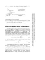
Figure 9.5.1. (a) Linear, quadratic, and cubic behavior at the roots of polynomials. Only under high
magnification (b) does it become apparent that the cubic has one, not three, roots, and that the quadratic
has two roots rather than none.
minus a few multiples of the machine precision at each stage) or unstably (erosion of
successive significant figures until the results become meaningless). Which behavior
occurs depends on just how the root is divided out. Forward deflation,wherethe
new polynomial coefficients are computed in the order from the highest power of x
down to the constant term, was illustrated in §5.3. This turns out to be stable if the
root of smallest absolute value is divided out at each stage. Alternatively, one can do
backward deflation, where new coefficients are computed in order from the constant
term up to the coefficient of the highest power of x. This is stable if the remaining
root of largest absolute value is divided out at each stage.
A polynomial whose coefficients are interchanged “end-to-end,” so that the
constant becomes the highest coefficient, etc., has its roots mapped into their
reciprocals. (Proof: Divide the whole polynomial by its highest power x

n
and
rewrite it as a polynomial in 1/x.) The algorithm for backward deflation is therefore
virtually identical to that of forward deflation, except that the original coefficients are
taken in reverse order and the reciprocal of the deflating root is used. Since we will
use forward deflation below, we leave to you the exercise of writinga concise coding
for backward deflation (as in§5.3). For more on the stability of deflation, consult
[2]
.
To minimize the impact of increasing errors (even stable ones) when using
deflation, it is advisable to treat roots of the successively deflated polynomials as
onlytentativerootsof theoriginalpolynomial. One then polishesthese tentativeroots
by taking them as initial guesses that are to be re-solved for, using the nondeflated
originalpolynomial P. Again you must beware lest two deflated roots are inaccurate
enough that, under polishing, they both converge to the same undeflated root; in that
case you gain a spurious root-multiplicity and lose a distinct root. This is detectable,
since you can compare each polished root for equality to previous ones from distinct
tentative roots. When it happens, you are advised to deflate the polynomial just
once (and for this root only), then again polish the tentative root, or to use Maehly’s
procedure (see equation 9.5.29 below).
Below we say more about techniques for polishing real and complex-conjugate
9.5 Roots of Polynomials
371
Sample page from NUMERICAL RECIPES IN C: THE ART OF SCIENTIFIC COMPUTING (ISBN 0-521-43108-5)
Copyright (C) 1988-1992 by Cambridge University Press.Programs Copyright (C) 1988-1992 by Numerical Recipes Software.
Permission is granted for internet users to make one paper copy for their own personal use. Further reproduction, or any copying of machine-
readable files (including this one) to any servercomputer, is strictly prohibited. To order Numerical Recipes books,diskettes, or CDROMs
visit website or call 1-800-872-7423 (North America only),or send email to (outside North America).
tentative roots. First, let’s get back to overall strategy.
There are two schools of thought about how to proceed when faced with a

polynomial of real coefficients. One school says to go after the easiest quarry, the
real, distinct roots, by the same kinds of methods that we have discussed in previous
sections for general functions, i.e., trial-and-error bracketing followed by a safe
Newton-Raphson as in rtsafe. Sometimes you are only interested in real roots, in
which case the strategy is complete. Otherwise, you then go after quadratic factors
of the form (9.5.1) by any of a variety of methods. One such is Bairstow’s method,
which we will discuss below in the context of root polishing. Another is Muller’s
method, which we here briefly discuss.
Muller’s Method
Muller’s method generalizes the secant method, but uses quadratic interpolation
among three points instead of linear interpolation between two. Solving for the
zeros of the quadratic allows the method to find complex pairs of roots. Given three
previous guesses for the root x
i−2
, x
i−1
, x
i
, and the values of the polynomial P (x)
at those points, the next approximation x
i+1
is produced by the following formulas,
q ≡
x
i
− x
i−1
x
i−1
− x

i−2
A ≡ qP(x
i
)− q(1 + q)P (x
i−1
)+q
2
P(x
i−2
)
B≡(2q +1)P(x
i
)−(1 + q)
2
P (x
i−1
)+q
2
P(x
i−2
)
C≡(1 + q)P (x
i
)
(9.5.2)
followed by
x
i+1
= x
i

− (x
i
− x
i−1
)

2C
B ±
√
B
2
− 4AC

(9.5.3)
where the sign in the denominator is chosen to make its absolute value or modulus
as large as possible. You can start the iterations with any three values of x that you
like, e.g., three equally spaced values on the real axis. Note that you must allow
for the possibility of a complex denominator, and subsequent complex arithmetic,
in implementing the method.
Muller’s method is sometimes also used for finding complex zeros of analytic
functions (not just polynomials) in the complex plane, for example in the IMSL
routine ZANLY
[3]
.
Laguerre’s Method
The second school regarding overall strategy happens to be the one to which
we belong. That school advises you to use one of a very small number of methods
that will converge (though with greater or lesser efficiency) to all types of roots:
real, complex, single, or multiple. Use such a method to get tentative values for all
n roots of your nth degree polynomial. Then go back and polish them as you desire.

372
Chapter 9. Root Finding and Nonlinear Sets of Equations
Sample page from NUMERICAL RECIPES IN C: THE ART OF SCIENTIFIC COMPUTING (ISBN 0-521-43108-5)
Copyright (C) 1988-1992 by Cambridge University Press.Programs Copyright (C) 1988-1992 by Numerical Recipes Software.
Permission is granted for internet users to make one paper copy for their own personal use. Further reproduction, or any copying of machine-
readable files (including this one) to any servercomputer, is strictly prohibited. To order Numerical Recipes books,diskettes, or CDROMs
visit website or call 1-800-872-7423 (North America only),or send email to (outside North America).
Laguerre’s method is by far the most straightforward of these general, complex
methods. It does require complex arithmetic, even while converging to real roots;
however, for polynomials with all real roots, it is guaranteed to converge to a
root from any starting point. For polynomials with some complex roots, little is
theoretically proved about the method’s convergence. Much empirical experience,
however, suggeststhatnonconvergence isextremely unusual,and, further, can almost
always be fixed by a simple scheme to break a nonconverging limit cycle. (This is
implemented in our routine, below.) An example of a polynomial that requires this
cycle-breaking scheme is one of high degree (
>
∼
20), with all its roots just outside of
the complex unit circle, approximately equally spaced around it. When the method
converges on a simple complex zero, it is known that its convergence is third order.
In some instances the complex arithmetic in the Laguerre method is no
disadvantage, since the polynomial itself may have complex coefficients.
To motivate (although not rigorously derive) the Laguerre formulas we can note
the following relations between the polynomial and its roots and derivatives
P
n
(x)=(x−x
1
)(x − x

2
) ...(x−x
n
)(9.5.4)
ln|P
n
(x)| =ln|x−x
1
|+ln|x−x
2
|+...+ln|x−x
n
| (9.5.5)
d ln|P
n
(x)|
dx
=+
1
x−x
1
+
1
x−x
2
+...+
1
x−x
n
=

P

n
P
n
≡G (9.5.6)
−
d
2
ln|P
n
(x)|
dx
2
=+
1
(x−x
1
)
2
+
1
(x−x
2
)
2
+...+
1
(x−x
n

)
2
=

P

n
P
n

2
−
P

n
P
n
≡ H (9.5.7)
Startingfrom these relations, the Laguerre formulas make what Acton
[1]
nicely calls
“a rather drastic set of assumptions”: The root x
1
that we seek is assumed to be
located some distance a from our current guess x, while all other roots are assumed
to be located at a distance b
x − x
1
= a ; x − x
i

= bi=2,3,...,n (9.5.8)
Then we can express (9.5.6), (9.5.7) as
1
a
+
n − 1
b
= G (9.5.9)
1
a
2
+
n− 1
b
2
= H (9.5.10)
which yields as the solution for a
a =
n
G ±

(n− 1)(nH − G
2
)
(9.5.11)
where the sign should be taken to yield the largest magnitude for the denominator.
Since the factor inside the square root can be negative, a can be complex. (A more
rigorous justification of equation 9.5.11 is in
[4]
.)

9.5 Roots of Polynomials
373
Sample page from NUMERICAL RECIPES IN C: THE ART OF SCIENTIFIC COMPUTING (ISBN 0-521-43108-5)
Copyright (C) 1988-1992 by Cambridge University Press.Programs Copyright (C) 1988-1992 by Numerical Recipes Software.
Permission is granted for internet users to make one paper copy for their own personal use. Further reproduction, or any copying of machine-
readable files (including this one) to any servercomputer, is strictly prohibited. To order Numerical Recipes books,diskettes, or CDROMs
visit website or call 1-800-872-7423 (North America only),or send email to (outside North America).
The method operates iteratively: For a trial value x, a is calculated by equation
(9.5.11). Then x − a becomes the next trial value. This continues until a is
sufficiently small.
The following routine implements the Laguerre method to find one root of a
given polynomial of degree m, whose coefficients can be complex. As usual, the first
coefficient a[0] is the constant term, while a[m] is the coefficient of the highest
power of x. The routine implements a simplified version of an elegant stopping
criterion due to Adams
[5]
, which neatly balances the desire to achieve full machine
accuracy, on the one hand, with the danger of iterating forever in the presence of
roundoff error, on the other.
#include <math.h>
#include "complex.h"
#include "nrutil.h"
#define EPSS 1.0e-7
#define MR 8
#define MT 10
#define MAXIT (MT*MR)
Here
EPSS
is the estimated fractional roundoff error. We try to break (rare) limit cycles with
MR

different fractional values, once every
MT
steps, for
MAXIT
total allowed iterations.
void laguer(fcomplex a[], int m, fcomplex *x, int *its)
Given the degree
m
and the
m+1
complex coefficients
a[0..m]
of the polynomial

m
i=0
a
[i]x
i
,
and given a complex value
x
, this routine improves
x
by Laguerre’s method until it converges,
within the achievable roundoff limit, to a root of the given polynomial. The number of iterations
taken is returned as
its
.
{

int iter,j;
float abx,abp,abm,err;
fcomplex dx,x1,b,d,f,g,h,sq,gp,gm,g2;
static float frac[MR+1] = {0.0,0.5,0.25,0.75,0.13,0.38,0.62,0.88,1.0};
Fractions used to break a limit cycle.
for (iter=1;iter<=MAXIT;iter++) { Loop over iterations up to allowed maximum.
*its=iter;
b=a[m];
err=Cabs(b);
d=f=Complex(0.0,0.0);
abx=Cabs(*x);
for (j=m-1;j>=0;j--) { Efficient computation of the polynomial and
its first two derivatives.f=Cadd(Cmul(*x,f),d);
d=Cadd(Cmul(*x,d),b);
b=Cadd(Cmul(*x,b),a[j]);
err=Cabs(b)+abx*err;
}
err *= EPSS;
Estimate of roundoff error in evaluating polynomial.
if (Cabs(b) <= err) return; We are on the root.
g=Cdiv(d,b); The generic case: use Laguerre’s formula.
g2=Cmul(g,g);
h=Csub(g2,RCmul(2.0,Cdiv(f,b)));
sq=Csqrt(RCmul((float) (m-1),Csub(RCmul((float) m,h),g2)));
gp=Cadd(g,sq);
gm=Csub(g,sq);
abp=Cabs(gp);
abm=Cabs(gm);
if (abp < abm) gp=gm;
dx=((FMAX(abp,abm) > 0.0 ? Cdiv(Complex((float) m,0.0),gp)

: RCmul(1+abx,Complex(cos((float)iter),sin((float)iter)))));
x1=Csub(*x,dx);