Innovations in Intelligent Machines 1 - Javaan Singh Chahl et al (Eds) Part 5 doc
Bạn đang xem bản rút gọn của tài liệu. Xem và tải ngay bản đầy đủ của tài liệu tại đây (587.43 KB, 20 trang )
70 P.B. Sujit et al.
0 20 40 60 80 100 120 140 160 180 200
0
0.5
1
1.5
2
2.5
3
3.5
4
4.5
x 10
4
Number of steps
Average total uncertainty
q = 1
Greedy
Security
Nash
Coalition
Cooperative
0 20 40 60 80 100 120 140 160 180 200
0
0.5
1
1.5
2
2.5
3
3.5
4
4.5
x 10
4
Number of steps
Average total uncertainty
q = 2
Greedy
Security
Nash
Coalition Nash
Cooperative
Fig. 9. Performance of various strategies for q = 1 and q = 2 averaged over 50 maps
and with same initial searcher positions
search operation and have values β
1
=0.5,β
2
=0.4,β
3
=0.6,β
4
=0.8, and
β
5
=0.7. We will study the performance of various game theoretical strategies
on total uncertainty reduction in a search space.
The simulation was carried out for 50 different uncertainty maps with the
same initial placement of agents and same total uncertainty in each map. The
positions of the searchers are as shown in Figure 8 and the total initial uncer-
tainty in each map is assumed to be 4.75 ×10
4
. The average total uncertainty
is the average of the total uncertainty for the 50 maps at each step, computed
up to a total of 200 search steps.
Figure 9 shows the comparative performance of various strategies with
different look ahead policies of q =1andq = 2. We can see that the average
total uncertainty reduces with each search step. The cooperative, noncoop-
erative Nash, and coalitional Nash strategies perform equally well and they
are better than the other strategies. From this figure we can see that for all
the search strategies, look ahead policy of q = 2 performs better than q =1,
which is expected.
However, with the increase in look ahead policy length the computational
time also increases significantly. Figure 10 gives the complete information
on the computational time requirements of each strategy for q =1and
q = 2. Since we consider 50 uncertainty maps, 5 agents, and 200 search steps,
there are 5 ×10
4
number of decision epochs involved in the complete simula-
tion. We plot the computational time needed by each decision epoch, where
(i-1) × 10
3
+1 to i × 10
3
decision epochs (marked on the vertical axis) are
the decisions taken for searching the i-th map. So each point on the graph
represents the time taken by the search algorithm to compute the search
effectiveness function (wherever necessary) and arrive at the route decision.
These computation times are obtained using a dedicated 3 GHz, P4 machine.
All decision epochs that take computation time ≤ 10
−3
seconds are plotted
against time 10
−3
seconds. The last plot in each set of graphs shows the dis-
tribution of computation times for various strategies in terms of the total
number of decision epochs that need computation time less than the value
Team, Game, and Negotiation based UAV Task Allocation 71
on the horizontal axis. These plots reveal important information about the
computational effort that each strategy demands.
Finally, we carried out another simulation to demonstrate the utility of
the Nash strategies when the perceived uncertainty maps of the agents are
different from the actual uncertainty map. For this it was assumed that the
uncertainty reduction factors (β) of the agents fluctuate with time due to
fluctuation in the performance of their sensor suites due to environmental
or other reasons. Each agent knows its own current uncertainty reduction
factor perfectly but assumes that the uncertainty reduction factors of the
other agents to be the same as their initial value. This produces disparity
in the uncertainty map between agents and from the actual uncertainty map
which evolves according to the true β values as the search progresses. The
variation in the value of β for the five agents are shown in Figure 11.
In this situation the total uncertainty reduction is as shown in Figure 12,
which shows that both the Nash strategies, which do not make any assumption
10
-3
10
-2
10
-1
10
0
10
1
10
2
2.8
3
3.2
3.4
3.6
3.8
4
4.2
4.4
4.6
4.8
5
x 10
4
Time in seconds
Number of decision epochs
q = 1
security
cooperative
greedy
Nash
Coalitional Nash
10
-3
10
-2
10
-1
10
0
10
1
10
2
4.2
4.3
4.4
4.5
4.6
4.7
4.8
4.9
5
x 10
4
Time in seconds
Number of decision epochs
q = 2
security
greedy
Nash & Coalitional Nash
Cooperative
Fig. 10. Computational time of various strategies for q = 2 for random initial
uncertainty maps
0 20 40 60 80 100 120 140
160
180 200
0.4
0.5
0.6
0.7
0.8
0.9
1
Number of steps
β
Variation of β with time steps
β
1
β
2
β
3
β
4
β
5
Fig. 11. Variation in the uncertainty reduction factors
72 P.B. Sujit et al.
0 20 40 60 80 100 120 140 160 180 200
1.5
2
2.5
3
3.5
4
4.5
5
x 10
4
Number of steps
Total uncertainty
q = 1
Greedy
Cooperative
Nash
Coalition Nash
0
20 40 60 80 100 120 140 160 180 200
1.5
2
2.5
3
3.5
4
4.5
5
x 10
4
Number of steps
Total uncertainty
q = 2
Greedy
Cooperative
Nash
Coalition Nash
Fig. 12. Performance in the non-ideal case with varying β
about the other agents’ actions, perform equally well and are also better than
the cooperative strategy which assumes cooperative behavior from the other
agents.
6 Conclusions
In this chapter, we addressed the problem of task allocation among auto-
nomous UAVs operating in a swarm using concepts from team theory, negoti-
ation, and game theory, and showed that effective and intelligent strategies can
be devised from these well-known theories to solve complex decision-making
problems in multi-agent systems. The role of communication between agents
was explicitly accounted for in the problem formulation. This is one of the
first use of these concepts to multi-UAV task allocation problems and we
hope that this framework and results will be a catalyst to further research in
this challenging area.
Acknowledgements
This work was partially supported by the IISc-DRDO Program on Advanced
Research in Mathematical Engineering.
References
1. C. Schumacher, P. Chandler, S. J. Rasmussen: Task allocation for wide area
search munitions via iterative netowrk flow, AIAA Guidance, Navigation, and
Control Conference and Exhibit, August, Monterey, California, 2002, AIAA
2002–4586
2. J.W. Curtis and R. Murphey: Simultaneaous area search and task assignment
for a team of cooperative agents, AIAA Guidance, Navigation, and Control
Conference and Exhibit, August, Austin, Texas, 2003, AIAA 2003–5584
Team, Game, and Negotiation based UAV Task Allocation 73
3. P.B. Sujit, A. Sinha, and D. Ghose: Multi-UAV task allocation using team the-
ory, Proc. of the IEEE Conference on Decision and Control, Seville, Spain,
December 2005, pp. 1497–1502
4. P.B. Sujit and D. Ghose, Multiple agent search in an unknown environment
using game theoretical models, Proc. of the American Control Conference,
Boston, pp. 5564–5569, 2004
5. P.B. Sujit and D. Ghose: Search by UAVs with flight time constraints using
game theoretical models, Proc. of the AIAA Guidance Navigation and Con-
trol Conference and Exhibit, San Francisco, California, August 2005, AIAA-
2005-6241
6. P.B. Sujit, A. Sinha and D. Ghose: Multiple UAV Task Allocation using Negotia-
tion, Proceedings of Fifth International joint Conference on Autonomous Agents
and Multiagent Systems, Japan, May. 2006 (to appear)
7. P.B. Sujit and D. Ghose: Multi-UAV agent based negotiation scheme, Proc. of
the American Control Conference, Portland, Oregon, June 2005, pp. 2995–3000
8. P.B. Sujit and D. Ghose: A self assessment scheme for multiple-agent search,
Proc. of the American Control Conference, Minneapolis, June 2006 (to appear)
9. K.E. Nygard, P.R. Chandler, M. Pachter: Dynamic network flow optimization
models for air vehicle resource allocation, Proc. of the the American Control
Conference, June 2001, Arlington, Texas, pp. 1853–1858
10. C. Schumacher, P. Chandler, M. Pachter, L.S. Pachter: UAV task assignment
with timing constraints, AIAA Guidance, Navigation, and Control Conference
and Exhibit, August, Austin, Texas, 2003, AIAA 2003–5664
11. C. Schumacher and P. Chandler: UAV task assignment with timing constraints
via mixed-integer linear programming, AIAA Unmanned Unlimited Techni-
cal Conference, Workshop and Exhibit, Chicago, Illinois, Sept. 2004, AIAA-
2004-6410
12. M. Alighanbari and J. How: Robust decentralized task assignment for coopera-
tive UAVs, AIAA Guidance, Navigation, and Control Conference and Exhibit,
Keystone, Colorado, Aug. 21–24, 2006
13. M. Darrah, W. Niland and B. Stolarik: UAV cooperative task assignments
for a SEAD mission using genetic algorithms, AIAA Guidance, Navigation,
and Control Conference and Exhibit, Keystone, Colorado, Aug. 2006, AIAA-
2006-6456
14. C. Schumacher, P.R. Chandler, S. J. Rasmussen, and D. Walker: Task allocation
for wide area search munitions with variable path length, Proc. of the American
Control Conference, June, Denver, Colorado, 2003, pp. 3472–3477
15. D. Turra, L. Pollini, and M. Innocenti: Real-time unmanned vehicles task alloca-
tion with moving targets, AIAA Guidance, Navigation, and Control Conference
and Exhibit, Providence, Rhode Island, August 2004, AIAA 2004–5253
16. Y. Jin, A. A. Minai, M. M. Polycarpou: Cooperative real-time search and task
allocation in UAV teams, IEEE Conference on Decision and Control,Maui,
Hawaii, December 2003, Vol. 1 , pp. 7–12
17. M.B. Dias and A. Stentz: A free market architecture for distributed control of
a multirobot system, 6th International Conference on Intelligent Autonomous
Systems, Venice, Italy, July 2000, pp. 115–122
18. M.B. Dias, R.M. Zlot, N. Kalra, and A. Stentz: Market-based multirobot coor-
dination: A survey and analysis, Technical report CMU-RI-TR-05-13, Robotics
Institute, Carnegie Mellon University, April 2005
74 P.B. Sujit et al.
19. B. Gerkey, and M.J. Mataric: Sold!: Auction methods for multi-robot control,
IEEE Transactions on Robotics and Automation, Vol. 18, No. 5, October 2002,
pp. 758–768
20. B. Gerkey, and M.J. Mataric: A formal framework for the study of task allocation
in multi-robot systems, International Journal of Robotics Research, Vol. 23,
No.9, Sep 2004, pp. 939–954
21. M.J. Mataric, G.S. Sukhatme, and E.H. Stergaard: Multi-robot task allocation
in uncertain environments, Autonomous Robots, Vol. 14, 2003, pp. 255–263
22. P. Gurfil: Evaluating UAV flock mission performance using Dudeks taxon-
omy, Proc. of the American Control Conference, Portland, Oregon, June 2005,
pp. 4679–4684
23. M. Lagoudakis, P. Keskinocak, A. Kleywegt, and S. Koenig: Auctions with per-
formance guarantees for multi-robot task allocation, Proc. of the IEEE Interna-
tional Conference on Intelligent Robots and Systems, Sendai, Japan, September
2004, pp. 1957–1962
24. S. Sariel and T. Balch: Real time auction based allocation of tasks for multi-
robot exploration problem in dynamic environments, AAAI workshop on Inte-
grating Planning into Scheduling, Pittsburgh, Pennsylvania, July 2005, Eds.
Mark Boddy, Amedeo Cesta, and Stephen F. Smith, pp. 27–33
25. J. Marschak: Elements for a theory of teams, Management Science,Vol.1,No.
2, Jan 1955, pp. 127–137
26. R. Radner: The linear team: An example of linear programming under uncer-
tainty, Proc. of 2nd Symposium in Linear Programming, Washington D.C, 1955,
pp. 381–396
27. S. Kraus: Automated negotiation and decision making in multiagent envi-
ronments, Multi-Agent Systems and Applications, Springer LNAI 2086, (Eds.)
M.Luck, V. Marik, O. Stepankova, and R. Trappl, 2001, pp. 150–172
28. A. Rubinstein: Perfect equilibrium in a bargaining model, Econometrica, Vol.
50, No. 1, 1982, pp. 97–109
29. K. Passino, M. Polycarpou, D. Jacques, M. Pachter, Y. Liu, Y. Yang, M. Flint,
and M. Baum: Cooperative control for autonomous air vehicles, Cooperative
Control and Optimization, (R. Murphey and P. M. Pardalos, eds.), vol. 66,
Kluwer Academic Publishers, 2002, pp. 233–271
30. R.F. Dell, J.N. Eagel, G.H.A. Martins, and A.G. Santos: Using multiple
searchers in constrained-path, moving-target search problems, Naval Research
Logistics, Vol. 43, pp. 463–480, 1996
31. T. Basar and G.J. Olsder: Dynamic Noncooperative Game Theory,Academic
press, CA 1995
32. S. Ganapathy and K.M. Passino: Agreement strategies for cooperative control
of uninhabited autonomous vehicles, Proc. of the American Control Conference,
Denver, Colorado, 2003, pp. 1026–1031
Author Biographies
P.B. Sujit has received his Bachelor’s Degree in Electrical Engineering from
the Bangalore University, MTech from Visveswaraya Technological University,
and PhD from the Indian Institute of Science, Bangalore. At present, he is a
Post Doctoral Fellow at Brigham Young University, Provo, Utah. His research
Team, Game, and Negotiation based UAV Task Allocation 75
interests include multi-agent systems, cooperative control, search theory, game
theory, economic models, and task allocation.
A. Sinha has received her Bachelor’s Degree in Electrical Engineering from
Jadavpur University, Kolkata, India, and MTech from Indian Institute of Tech-
nology, Kanpur, India. At present she is a graduate student at the Department
of Aerospace Engineering, Indian Institute of Science, Bangalore, India. Her
research interests include cooperative control of autonomous agents, team the-
ory, and game theory.
D. Ghose is a Professor in the Department of Aerospace Engineering at the
Indian Institute of Science, Bangalore, India. He obtained a BSc(Engg) degree
from the National Institute of Technology (formerly the Regional Engineer-
ing College), Rourkela, India, in 1982, and an ME and a PhD degree, from
the Indian Institute of Science, Bangalore, in 1984 and 1990, respectively.
His research interests are in guidance and control of aerospace vehicles, col-
lective robotics, multiple agent decision-making, distributed decision-making
systems, and scheduling problems in distributed computing systems. He is an
author of the book Scheduling Divisible Loads in Parallel and Distributed Sys-
tems published by the IEEE Computer Society Press (presently John Wiley).
He is in the editorial board of the IEEE Transactions on Systems, Man, and
Cybernetics, Part A: Systems and Humans, and the IEEE Transactions on
Automation Science and Engineering. He has held visiting positions at the
University of California at Los Angeles and several other universities. He is
an elected fellow of the Indian National Academy of Engineering.
UAV Path Planning Using Evolutionary
Algorithms
Ioannis K. Nikolos, Eleftherios S. Zografos, and Athina N. Brintaki
Department of Production Engineering and Management,
Technical University of Crete, University Campus,
Kounoupidiana, GR-73100, Chania, Greece
Abstract. Evolutionary Algorithms have been used as a viable candidate to solve
path planning problems effectively and provide feasible solutions within a short time.
In this work a Radial Basis Functions Artificial Neural Network (RBF-ANN) assisted
Differential Evolution (DE) algorithm is used to design an off-line path planner for
Unmanned Aerial Vehicles (UAVs) coordinated navigation in known static maritime
environments. A number of UAVs are launched from different known initial locations
and the issue is to produce 2-D trajectories, with a smooth velocity distribution along
each trajectory, aiming at reaching a predetermined target location, while ensuring
collision avoidance and satisfying specific route and coordination constraints and
objectives. B-Spline curves are used, in order to model both the 2-D trajectories
and the velocity distribution along each flight path.
1 Introduction
1.1 Basic Definitions
The term unmanned aerial vehicle or UAV, which replaced in the early 1990s
the term remotely piloted vehicle (RPV), refers to a powered aerial vehicle
that does not carry a human operator, uses aerodynamic forces to provide
vehicle lift, can fly autonomously or be piloted remotely, can be expendable
or recoverable, and can carry a lethal or non lethal payload [1]. UAVs are
currently evolving from being remotely piloted vehicles to autonomous robots,
although ultimate autonomy is still an open question.
The development of autonomous robots is one of the major goals in Robot-
ics [2]. Such robots will be capable of converting high-level specification of
tasks, defined by humans, to low-level action algorithms, which will be exe-
cuted in order to accomplish the predefined tasks. We may define as plan this
sequence of actions to be taken, although it may be much more complicated
than that. Motion planning (or trajectory planning) is one category of such
I.K. Nikolos et al.: UAV Path Planning Using Evolutionary Algorithms, Studies in Computa-
tional Intelligence (SCI) 70, 77–111 (2007)
www.springerlink.com
c
Springer-Verlag Berlin Heidelberg 2007
78 I.K. Nikolos et al.
problems. Besides the great variety of planning problems and models found
in Robotics, some basic terms are common throughout the entire subject.
The state space includes all possible situations that might arise during
the planning procedure. In the case of an UAV each state could represent its
position in physical space, along with its velocity. The state space could be
either discrete or continuous; motion planning is planning in continuous state
spaces. Although its definition is an important component of the planning
problem formulation, in most cases is implicitly represented, due to its large
size [3].
Planning problems also involve the time dimension. Time may be explicitly
or implicitly modeled and may be either discrete or continuous, depending
on the planning problem under consideration. However, for most planning
problems, time is implicitly modeled by simply specifying a path through a
continuous space [3].
Each state in the state space changes through a sequence of specific actions,
included in the plan. The connection between actions and state changes should
be specified through the use of proper functions or differential equations.
Usually, these actions are selected in a way to “move” the object from an
initial state to a target or goal state.
A planning algorithm may produce various different plans, which should
be compared and valued using specific criteria. These criteria are generally
connected to the following major concerns, which arise during a plan gen-
eration procedure: feasibility and optimality. The first concern asks for the
production of a plan to safely “move” the object to its target state, without
taking into account the quality of the produced plan. The second concern asks
for the production of optimal, yet feasible, paths, with optimality defined in
various ways according to the problem under consideration [3]. Even in simple
problems searching for optimality is not a trivial task and in most cases results
in excessive computation time, not always available in real-world applications.
Therefore, in most cases we search for suboptimal or just feasible solutions.
Motion planning usually refers to motions of a robot (or a collection of
robots) in the two-dimensional or three-dimensional physical space that con-
tains stationary or moving obstacles. A motion plan determines the appropri-
ate motions to move the robot from the initial to the target state, without
colliding into obstacles. As the state space in motion planning is continuous, it
is uncountably infinite. Therefore, the representation of the state space should
be implicit. Furthermore, a transformation is often used between the real world
where the robots are moving and the space in which the planning takes place.
This state space is called the configuration space (C-space) and motion plan-
ning can be defined as a search for a continuous path in this high-dimensional
configuration space that ensures collision avoidance with implicitly defined
obstacles. However, the use of configuration space is not always adopted and
the problem is formulated in the physical space; especially in cases with con-
stantly varying environment (as in most of UAV applications) the use of confi-
guration space results in excessive computation time, which is not available in
UAV Path Planning Using Evolutionary Algorithms 79
real-time in-flight applications. Path planning is the generation of a space path
between an initial location and the desired destination that has an optimal or
near-optimal performance under specific constraints [4]. A detailed descrip-
tion of motion and path planning theory and classic methodologies can be
found in [2] and in [3].
1.2 Cooperative Robotics
The term collective behavior denotes any behavior of agents in a system of
more than a single agent. Cooperative behavior is a subclass of collective behav-
ior which is characterized by cooperation [5]. Research in cooperative Robot-
ics has gained increased interest since the late 1980’s, as systems of multiple
robots engaged in cooperative behavior show specific benefits compared to a
single robot [5]:
• Tasks may be inherently too complex, or even impossible, for a single
robot to accomplish, or the performance is enhanced if using multiple
agents, since a single robot, despite its capabilities and characteristics, is
spatially limited.
• Building or using a system of simpler robots may be easier, cheaper,
more flexible and more fault-tolerant than using a single more compli-
cated robot.
In [5] cooperative behavior is defined as follows: Given some tasks specified
by a designer, a multiple robot system displays cooperative behavior if, due
to some underlying mechanism, i.e. the “mechanism of cooperation”, there is
an increase in the total utility of the system.
Geometric problems arise when dealing with cooperative moving robots,
as they are made to move and interact with each other inside the physical 2D
or 3D space. Such geometric problems include multiple-robot path planning,
moving to and maintaining formation, and pattern generation [5].
According to Fujimura [6], path planning can be either centralized or distri-
buted. In the first case a universal path planner makes all decisions. In the sec-
ond case each agent plans and adjusts its path. Furthermore, Arai and Ota [7]
allow for hybrid systems that are combinations of on-line, off-line, centralized,
or decentralized path planners. According to Latombe [2], centralized planning
takes into account all robots, while decoupled planning corresponds to indep-
endent computation of each robot’s path. Methods originally used for single
robots can be also applied to centralized planning. For decoupled planning
two approaches were proposed: a) prioritized planning, where one robot at a
time is considered, according to a global priority, and b) path coordination,
where the configuration space-time resource is appropriately scheduled to plan
the paths.
Cooperation of UAVs has gained recently an increased interest due to the
potential use of such systems for fire fighting applications, military missions,
80 I.K. Nikolos et al.
search and rescue scenarios or exploration of unknown environments (space-
oriented applications). In order to establish a reliable and efficient frame-
work for the cooperation of a number of UAVs several problems have to be
encountered:
• UAV task assignment problem: a number of UAVs is required to per-
form a number of tasks, with predefined order, on a number of targets.
The requirements for a feasible and efficient solution include taking into
account: task precedence and coordination, timing constraints, and flyable
trajectories [8]. The task re-assignment problem should be also considered,
in order to take into account possible failure of a UAV to accomplish its
task. The task assignment problem is a well-known optimization problem;
it is NP-hard and, consequently, heuristic techniques are often used.
• UAV path planning problem: a path planning algorithm should provide
feasible, flyable and near optimal trajectories that connect starting with
target points. The requirement for feasible trajectories dictates collision
avoidance between the cooperating UAVs as well as between the vehicles
and the ground. The requirement of flyable trajectories usually dictates
a lower bound on the turn radius and speed of the UAVs [8]. Addition-
ally, an upper bound for the speed of each UAV may be required. The
path optimality can be defined in various ways, according to the mission
assigned. However, a typical requirement is to minimize the total length
of the paths.
• Data exchange between cooperating UAVs and data fusion: exchange
of information between cooperating UAVs is expected to enhance the
effectiveness of the team. However, in real world applications communica-
tion imperfections and constraints are expected, which will cause coordi-
nation problems to the team [9]. Decentralized implementations of the
decision and control algorithms may reduce the sensitivity to communi-
cation problems [10].
• Cooperative sensing of the targets: the problem is defined as how to
co-operate the UAV sensors in terms of their locations to achieve optimal
estimation of the state of each target [11] (a target localization problem).
• Cooperative sensing of the environment: the problem is defined as how
to cooperate the UAV sensors in order to achieve better awareness of
the environment (popup threats, changing weather conditions, moving
obstacles etc.). In this category we may include the coordinated search of
a geographic region [12].
1.3 Path Planning for Single and Multiple UAVs
Compared to the path-planning problem in other applications, path planning
for UAVs has some of the following characteristics, according to the mission
[13, 14, 15]:
UAV Path Planning Using Evolutionary Algorithms 81
• Stealth, in order to minimize the probability of detection by hostile radar,
by flying along a route which keeps away from possible threats and/or has
a lower altitude to avoid radar detection.
• Physical feasibility, which refers to the physical (or technology) limitations
from the use of UAVs, such as limited range, minimum turning angle,
minimum and maximum speed etc.
• Performance of mission, which imposes special requirements, including
maximum turning angle, maximum climbing/diving angle, minimum and/
or maximum flying altitude and specific approaching angle to the target
point.
• Cooperation between UAVs in order to maximize the possibility of mission
accomplishment.
• Real-time implementation, which asks for computationally efficient
algorithms.
The characteristics above imply special issues that have to be consi-
dered for an efficient modeling of the (single or multiple) UAV path planning
problems.
Path modeling:
The simpler way to model an UAV path is by using straight-line segments
that connect a number of way points, either in 2D or 3D space [12, 15]. This
approach takes into account the fact that in typical UAV missions the shortest
paths tend to resemble straight lines that connect way points with starting
and target points and the vertices of obstacle polygons. Although way points
can be efficiently used for navigating a flying vehicle, straight-line segments
connecting the corresponding way points cannot efficiently represent the real
path that will be followed by the vehicle. As a result, these simplified paths
cannot be used for an accurate simulation of the movement of the UAV in
an optimization procedure, unless a large number of way points is adopted.
In that case the number of design variables in the optimization procedure
explodes, along with the computation time. The problem becomes even more
difficult in the case of cooperating flying vehicles.
In [16], paths from the initial vehicle location to the target location
are derived from a graph search of a Voronoi diagram that is constructed
from the known threat locations. The resulting paths consist of line segments.
These paths are subsequently smoothed around each way point, in order to
provide feasible trajectories within the dynamic constraints of the vehicle. A
great advantage of the Voronoi diagram approach is that it reduces the path
planning problem from an infinite dimensional search, to a finite-dimensional
graph search. This important abstraction makes the path planning problem
feasible in near-real time, even for a large number of way points [16].
Vandapel et al. [17] used a network of free space bubbles to model the
path of small scale UAVs, in order to solve the path planning problem of
autonomous unmanned aerial navigation below the forest canopy. Using a
82 I.K. Nikolos et al.
priori aerial data scans of forest environments, they compute a network of
free space bubbles, which form safe paths within the forest environment.
Their approach is tailored to the problem of small scale UAVs and can be
decomposed into two steps: 1) the scene made of 3-D points is segmented
into three classes (ground, vegetation and tree trunk-branches). 2) A path
planning algorithm explores the segmented environment and computes con-
nected obstacle-free areas, which will subsequently form a network of tunnels
intersecting at some locations.
An alternative approach is to model the UAV dynamics using the Dubins
car formulation [18]. The UAV is assumed to fly with constant altitude,
constant flight speed and to have continuous time kinematics [19]. This
approach cannot efficiently model real world scenarios, which may include
3D terrain avoidance or following of stealthy routes. However, this approach
seems to be sufficient enough for task assignment purposes to cooperating
UAVs flying at safe altitudes [19, 8, 20].
B-Spline curves have been used for trajectory representation in 2-D
environments (simulated annealing based path line optimization, combined
with fuzzy logic controller for path tracking) [21], and in 3-D environments
(Evolutionary Algorithm based path line optimization for a UAV over rough
terrain) [22, 23]. B-Spline curves need a few variables (the coordinates of
their control points) in order to define complicated 2D or 3D curved paths,
providing at least first order derivative continuity. Each control point has a
very local effect on the curve’s shape and small perturbations in its position
produce changes in the curve only in the neighborhood of the repositioned
control point.
Cooperation Scenarios:
Path planning algorithms were initially developed for the solution of the prob-
lem of a single UAV. The increasing interest for missions involving cooperating
UAVs resulted in the development of algorithms that take into account the
special characteristics and constraints of such missions. The related works
present various scenarios, formulations and approaches connected to cooper-
ating UAV path planning problems. Some of the most representative scenarios
are presented below.
Beard et al. [16] considered the scenario where a group of UAVs is required
to transition through a number of known target locations, with a number
of threats in the region of interest. Some threats are known a priori, some
others “pop up” or become known only when a UAV flies near them. It is
desirable to have multiple UAVs arrive on the boundary of each target’s radar
detection region simultaneously. Collision avoidance is ensured by supposing
that individual UAVs fly at different pre-assigned altitudes. In this work the
problem is decomposed in several sub-problems: a) The assignment problem
of a number of UAVs to a number of targets in a way that each target has
multiple UAVs assigned to it, with a high preference to specific targets. b) The
UAV Path Planning Using Evolutionary Algorithms 83
determination for each team of UAVs assigned to a target of an estimated time
over target that ensures simultaneous intercept and is feasible for all UAVs
in the team. c) The determination of a path (specified via waypoints) that
can be completed within the specified time over target, taking into account
minimum and maximum velocity constraints. d) The transformation of the
initial path into a feasible UAV trajectory. e) The development of controllers
for each UAV to track their computed trajectory.
A simpler scenario is presented in [15], where the problem under consider-
ation is to generate routes for cooperating UAVs in real time, which take into
account the exposure of UAVs to the threats and enable the vehicles to arrive
at their goal location simultaneously. Some of the threats are known a priori,
some of them “pop up” or become known only when a UAV approaches to it.
For each UAV are imposed minimum and maximum velocity constraints. The
cooperation related constraints are: a) the simultaneous arrival of all UAVs
at goal locations, and b) the collision avoidance between UAVs.
In [20] the motion-planning problem for a limited resource of mobile sensor
agents (MSAs) is investigated, in an environment with a number of targets
larger than the available MSAs. The MSAs are assumed to move much faster
than the targets. In order to keep the targets in surveillance the members
of the MSA team have to fly back and forth to update the targets’ status.
This NP-hard problem is essentially a combination of the problems of sensor
resource management and robot motion planning. The problem is formulated
as an optimization problem whose objective is to minimize the average time
duration between two consecutive observations of each target.
In [12] the objective is to provide a coordinated plan for searching a geo-
graphic region, represented by a grid of cells, using a team of searchers. Each
cell is characterized by its elevation and a cost parameter that corresponds to
the danger of visiting it. Each vehicle carries a sensor, characterized by scan
radius, angle and direction. The mission objective is the target coverage, i.e.
the percentage of the region that must be scanned during the mission. Scans
can be performed only from safe cells (the cell and all 8 neighbors should
have been previously scanned). Additionally the path that connects scanning
points should traverse through already scanned cells (a soft constraint). For
safety reasons scanning paths are not allowed to be very close to each other.
Solution methodologies:
Path planning problems are actually multi-objective multi-constraint optimi-
zation problems, in most cases very complex and computationally demanding
[24]. The problem complexity increases when multiple UAVs should be used.
Various approaches have been reported for UAVs coordinated route planning,
such as Voronoi diagrams [16], mixed integer linear programming [25, 26] and
dynamic programming [27] formulations.
In [25, 26] mixed-integer linear programming (MILP) is used to solve
tightly-coupled task assignment problems with timing constraints. The
84 I.K. Nikolos et al.
advantage to this approach is that it yields the optimal solution for the given
problem. The primary disadvantage is the high computational time required.
In [16] the motion-planning problem was decomposed into a waypoint path
planner and a dynamic trajectory generator. The path-planning problem was
solved via a Voronoi diagram and Eppstein’s k-best paths algorithm. The
trajectory generator problem was solved via a real-time nonlinear filter that
explicitly accounts for the dynamic constraints of the vehicle and modifies
the initial path. This decomposition of the motion-planning problem has the
advantage of decomposing a non-polynomial optimization problem into two
sub-problems that can be computed in near-real time, with the disadvantage
of providing a suboptimal solution [16].
Computational intelligence methods, such as Neural Networks [28], Fuzzy
Logic [29] and Evolutionary Algorithms (EAs) [15, 23] (or, in some cases, a
combination of them) have been successfully used in the development of algo-
rithms that produce trajectories for guiding mobile robots in known, unknown
or partially known environments.
During the past few years, it has been shown by many researchers that
EAs are a viable candidate to solve path planning problems effectively and
provide feasible solutions within a short time without demanding excessive
computer power. The reasons behind choosing EAs as an optimization tool
for the path-planning problem are their high robustness compared to other
existing directed search methods, their ease of implementation in problems
with a relatively high number of constraints, and their high adaptability to
the special characteristics of the problem under consideration [23].
Traditionally, EAs have been used for the solution of the path-finding
problem in ground based or sea surface navigation [30]. Commonly, the gen-
erated trajectory composed of straight line segments, connecting successive
way points, that guided a mobile robot or a vehicle along a 2-D path on the
earth’s or sea’s surface. The design variables used represented the coordinates
of the way points, where the vehicle changes its direction. Other approaches
took into account the time dimension by using design variables that also
described the vehicle steady speed as it traversed a part of its path. When the
vehicle’s operational environment was partially known or dynamic, a feasible
and safe trajectory was planned off-line by the EA, and the algorithm was
used on-line whenever unexpected obstacles were sensed [31, 32]. EAs have
been also used for solving the path-finding problem in a 3-D environment for
underwater vehicles, assuming that the path is a sequence of cells in a 3-D
grid [33, 34].
In [23] an EA based framework was utilized to design an off-line/on-line
path planner for UAVs autonomous navigation. The path planner calculates
a curved path line, represented using B-Spline curves in a 3-D rough terrain
environment; the coordinates of B-Spline control points serve as design vari-
ables. The off-line planner produces a single B-Spline curve that connects
the starting and target points with a predefined initial direction. The on-line
planner gradually produces a smooth 3-D trajectory aiming at reaching a
UAV Path Planning Using Evolutionary Algorithms 85
predetermined target in an unknown environment; the produced trajectory
consists of smaller B-Spline curves smoothly connected with each other. For
both off-line and on-line planners, the problem is formulated as an optimiza-
tion one; each objective function is formed as the weighted sum of different
terms, which take into account the various objectives and constraints of the
corresponding problem. Constraints are formulated using penalty functions.
Changwen Zheng et al. [15] proposed a route planner for UAVs, based
on evolutionary computation, which can be used to plan routes for either
single or multiple vehicles. The flight route consists of straight-line segments,
connecting the way points from the starting to the goal points. A real coded
chromosome representation is used; for each way point its physical coordinates
are used as design variables, along with a state variable, which provides infor-
mation on the feasibility of the corresponding way point and the feasibility
of the route segment connecting the point to the next one. The cost func-
tion of flight route penalizes the length of the route, penalizes flight routes at
high altitudes and routes that come dangerously close to known ground threat
sites. The imposed constraints on route segments are relevant to: minimum
route leg length, maximum route distance, minimum flying height, maximum
turning angle, maximum climbing/diving angle, simultaneous arrival at tar-
get location and no collision between vehicles. The route planning problem
is formulated as the problem of minimization of the cost function under the
aforementioned constraints.
In [8] a multi-task assignment problem for cooperating UAVs is formulated
as a combinatorial optimization problem. A Genetic Algorithm is utilized for
assigning the multiple agents to perform multiple tasks on multiple targets.
The algorithm allows efficiently solving this NP-hard problem and, addition-
ally, allows taking into account requirements such as task precedence and
coordination, timing constraints, and flyable trajectories. The performance
metric for the optimization problem is defined as the cumulative distance
traveled by the vehicles to perform all of the required tasks; the objective is
to minimize this metric subject to the above requirements. Integer encoding
is used for the chromosomes, which are composed of two rows; the first row
presents the assignment of a vehicle to perform a task on the target appear-
ing on the second row. The algorithm was compared to a stochastic random
search and a deterministic branch and bound search methods and found to
provide near optimal solutions considerably faster than the other methods.
1.4 Outline of the Current Work
The following scenario was considered in this work: Assuming a number of
UAVs at different known initial locations, the issue is to produce 2-D tra-
jectories, with a desirable velocity distribution along each trajectory, reach-
ing a common target under specific coordination and route constraints. The
constraints and objectives refer to: minimum path lengths, collision avoid-
ance between the flying vehicles and the ground, predefined minimum and
86 I.K. Nikolos et al.
maximum UAV velocity magnitudes during their flights, predefined safety
distance between UAVs, near simultaneous arrival to the target and target
approach from different directions.
This work is an extension of a previous one [35], which used Differential
Evolution (DE) in order to find optimal paths of coordinated UAVs, with
the paths being modeled with straight line segments. The main drawback of
that approach was the need of a large number of segments for complicated
paths, resulting in a large number of design variables and, consequently, gen-
erations to converge. In this work the Differential Evolution (DE) algorithm is
combined with a Radial Basis Functions Network (RBFN), which serves as a
surrogate approximation, in order to reduce the number of exact evaluations
of candidate solutions. The candidate paths are modeled in the physical space
and evaluated with respect to the physical (working) space. B-Spline curves
are used for path line modeling, and complicated paths can be produced with
a small number of control variables.
The rest of the chapter is organized as follows: section 2 contains
B-Spline and Evolutionary Algorithms fundamentals; the solid terrain formu-
lation, used for experimental simulations, is also presented. An off-line path
planner for a single UAV will be briefly discussed in section 3, in order to
introduce the concept of UAV path planning using Evolutionary Algorithms.
Section 4 deals with the concept of coordinated UAV path planning using
Evolutionary Algorithms. The problem formulation is described, including
assumptions, objectives, constraints, objective function definition and path
modeling. Section 5 presents the optimization procedure using a combination
of Differential Evolution and a Radial Basis Functions Artificial Neural Net-
work, which is used as a surrogate model in order to enhance the converge
rate of Differential Evolution algorithm. Simulations results are presented in
section 6, followed by discussion and conclusions in section 7.
2 B-Spline and Evolutionary Algorithms Fundamentals
2.1 B-Spline Curves
Straight-line segments cannot represent a flying objects path line, as it is
usually the case with mobile robots, sea and undersea vessels. B-Splines are
adopted to define the UAV desired path, providing at least first order deriva-
tive continuity. B-Spline curves are well fitted in the evolutionary procedure;
they need a few variables (the coordinates of their control points) in order to
define complicated curved paths. Each control point has a very local effect on
the curve’s shape and small perturbations in its position produce changes in
the curve only in the neighborhood of the repositioned control point.
B-Spline curves are parametric curves, with their construction based on
blending functions [36, 37]. Their parametric construction provides the ability
UAV Path Planning Using Evolutionary Algorithms 87
to produce non-monotonic curves. If the number of control points of the cor-
responding curve is n + 1, with coordinates (x
0
,y
0
,z
0
), ,(x
n
,y
n
,z
n
), the
coordinates of the B-Spline curve may be written as
x (u)=
n
i=0
x
i
· N
i,p
(u) , (1)
y (u)=
n
i=0
y
i
· N
i,p
(u) , (2)
z (u)=
n
i=0
z
i
· N
i,p
(u) , (3)
where u is the free parameter of the curve, N
i,p
(u) are the blending functions
of the curve and p is its degree, which is associated with curve’s smoothness
(p + 1 being its order). Higher values of p correspond to smoother curves.
The blending functions are defined recursively in terms of a knot vector
U = {u
0
, ,u
m
}, which is a non-decreasing sequence of real numbers, with
the most common form being the uniform non-periodic one, defined as
u
i
=
⎧
⎨
⎩
0 if i < p +1
i − pifp+1≤ i ≤ n
n − p +1 if n < i.
(4)
The blending functions N
i,p
are computed, using the knot values defined
above, as
N
i,0
(u)=
1 if u
i
≤ u<u
i+1
0 otherwise,
(5)
N
i,p
(u)=
u − u
i
u
i+p
− u
i
N
i,p−1
(u)+
u
i+p+1
− u
u
i+p+1
− u
i+1
N
i+1,p−1
(u) . (6)
If the denominator of either of the fractions is zero, that fraction is defined
to have zero value. Parameter u varies between 0 and (n−p+1) with a constant
step, providing the discrete points of the B-Spline curve. The sum of the values
of the blending functions for any value of u is always 1.
The use of B-Spline curves for the determination of a flight path provides
the advantage of describing complicated non-monotonic 3-dimensional curves
with controlled smoothness with a small number of design parameters, i.e.
the coordinates of the control points. Another valuable characteristic of the
adopted B-Spline curves is that the curve is tangential to the control polygon
at the starting and ending points. This characteristic can be used in order to
define the starting or ending direction of the curve, by inserting an extra fixed
point after the starting one, or before the ending control point. Figure 1 shows
a quadratic 2-dimensional B-Spline curve (p = 2) with its control points and
the corresponding control polygon.
88 I.K. Nikolos et al.
Fig. 1. A quadratic (p = 2) 2-dimensional B-Spline curve, produced using a uniform
non-periodic knot vector, and its control polygon
2.2 Fundamentals of Evolutionary Algorithms (EAs)
EAs are a class of search methods with remarkable balance between exploita-
tion of the best solutions and exploration of the search space. They combine
elements of directed and stochastic search and, therefore, are more robust
than directed search methods. Additionally, they may be easily tailored to
the specific application of interest, taking into account the special character-
istics of the problem under consideration [38, 39, 30].
The natural selection process is simulated in EAs, using a number (popu-
lation) of individuals (candidate solutions to the problem) to evolve through
certain procedures. Each individual is represented through chromosome -a
string of numbers (bit strings, integers or floating point numbers), in a sim-
ilar way with chromosomes in nature; it contains the design variables of the
optimization problem. Each individual’s quality is represented by a fitness
function tailored to the problem under consideration.
Classic Genetic Algorithms (GAs) use binary coding for the representation
of the genotype. However, floating point coding moves EAs closer to the prob-
lem space, allowing the operators to be more problem specific; this provides a
better physical representation of the space constraints. Additionally, directed
search techniques gain physical meaning and they are easily applicable.
In general, EA starts by generating, randomly, the initial chromosome
population with their genes (the design variables in the case of floating point
coding) taking values inside the desired constrained space of each design vari-
able. The lower and higher constraints of each gene may be chosen in a way
that specific undesirable solutions may be avoided. Although the shortening of
the search space reduces the computation time, it may also lead to sub-optimal
solutions, due to the lower variability between the potential solutions.
UAV Path Planning Using Evolutionary Algorithms 89
After the evaluation of each individual’s fitness function, operators are
applied to the population, simulating the according natural processes. Applied
operators include various forms of recombination, mutation and selection,
which are used in order to provide the next generation chromosomes. The
first classic operator applied to the selected chromosomes is the one-point
crossover scheme. Two randomly selected chromosomes are divided in the
same (random) position, while the first part of the first one is connected to
the second part of the second one and vice-versa. The crossover operator is
used to provide information exchange between different potential solutions to
the problem.
The second classic operator applied to the selected chromosomes is the uni-
form mutation scheme. This asexual operator alters a randomly selected gene
of a chromosome. The new gene takes its random value from the constrained
space, determined in the beginning of the process. The mutation operator is
used in order to introduce some extra variability into the population.
The resulting intermediate population is evaluated and a fitness function is
assigned to each member of the population. Using a selection procedure (diff-
erent for each type of EA) the best individuals of the intermediate population
(or the best individuals of the intermediate and the previous population) will
form the next generation. The process of a new generation evaluation and
creation is successively repeated, providing individuals with high values of
fitness function.
2.3 The Solid Boundary Representation
In the simulation results that will be presented the terrain where UAVs fly is
represented by a meshed 3-D surface, produced using mathematical functions
of the form
z (x, y)=sin(y + a)+b · sin (x)+c · cos
d ·
x
2
+ y
2
+ e · cos (y)+f · sin
f ·
x
2
+ y
2
+ g ·cos (y) , (7)
where a, b, c, d, e, f, g are constants experimentally defined, in order to
produce either a surface with mountains and valleys (as shown in Fig. 2) or a
maritime environment with islands close to each other (as shown in Fig. 6).
A graphical interface has been developed for the visualization of the terrain
surface, along with the path lines [23]. The corresponding interface deals with
different terrains produced either artificially or based on real geographical
data, providing an easy verification of the feasibility and the quality of each
solution. The path-planning algorithm considers the boundary surface as a
group of quadratic mesh nodes with known coordinates.
90 I.K. Nikolos et al.
Fig. 2. A typical simulation result of the off-line path planner for a single UAV;
the horizontal section of the terrain represents the imposed upper limit to the UAV
flight. The starting position is marked with a circle
3 Off-line Path Planner for a Single UAV
The off-line path planner, discussed in detail in [23], will be briefly presented
here, in order to introduce the concept of UAV path planning using Evo-
lutionary Algorithms. The off-line planner generates collision free paths in
environments with known characteristics and flight restrictions. The derived
path line is a single continuous 3-D B-Spline curve, while the solid bound-
aries are interpreted as 3-D rough surfaces. The starting and ending control
points of the B-Spline curve are fixed. A third point close to the starting one
is also fixed, determining the initial flight direction. Between the fixed control
points, free-to-move control points determine the shape of the curve, taking
values in the constrained space. The number of the free-to-move control points
is user-defined. Their physical coordinates are the genes of the EA artificial
chromosome.
The optimization problem to be solved minimizes a set of four terms,
connected to various objectives and constraints; they are associated with the
feasibility and the length of the curve, a safety distance from the obstacles and
the UAV’s flight envelope restrictions. The objective function to be minimized
is defined as
f =
4
i=1
w
i
f
i
. (8)
Term f
1
penalizes the non-feasible curves that pass through the solid
boundary. The penalty value is proportional to the number of discretized curve