Mechanics of Microelectromechanical Systems - N.Lobontiu and E.Garcia Part 8 pot
Bạn đang xem bản rút gọn của tài liệu. Xem và tải ngay bản đầy đủ của tài liệu tại đây (889 KB, 30 trang )
198
Chapter 4
In the majority of MEMS applications‚ the actuation force or the sensing
signal are insufficient when only one pair of moving-fixed parts are being
utilized. The practical solution to this problem is to couple several pairs of
such mating members in a comb-type configuration. Figure 4.19 sketches an
interdigitated pair with the main geometric parameters. The motion about
direction 1 in this figure is usually referred to as parallel-plate whereas the
other possible motion‚ about direction 2‚ is generally named comb-finger
motion. However‚ the interdigitated designs are used for both motions‚ and
therefore‚ in order to avoid confusion‚ the alternative denominations of
transverse and longitudinal will be used to indicate motions about the 1 and
2 directions‚ respectively.
These two types of motions are the main technological applications in
planar MEMS‚ and they will be presented in the following sub-sections. The
potentially-variable distances between the moving and fixed parts are the
gaps‚ denoted by and in Fig. 4.19 in order to indicate the axis they refer
to. Similarly‚ the thickness of a fixed/free member is indicated by either or
depending on the axis. These two main directions of transductions are
better indicated in Fig. 4.20. The guided supports are just a notional
representation because pure roller bearings are rare in MEMS design. The
motion directionality is rather achieved by using a proper spring suspension‚
as the ones studied in the previous chapter.
Figure 4.20 Main electrostatic linear transduction motions: (a) Transverse; (b) Longitudinal
The transverse and longitudinal transduction principles will be presented
next‚ as well as another electrostatic method which uses microcantilevers for
out-of-the-plane actuation/sensing. It should be mentioned that the purpose
of studying the actuation is to define the actuation force that is produced
electrostatically‚ whereas the objective of characterizing the sensing is to
determine the capacitance variation as a function of the changing in gap.
Figure 4.21 is the picture of a transverse electrostatic sensing device that was
fabricated by the MUMPs technology. The upper row of plates is mobile
whereas the two rows at the bottom of the figure support the fixed plates. It
can be seen that a pair of fixed plates is placed between two mobile plates in
4.
Microtransduction: actuation and sensing
199
this design‚ which creates a differential sensing capacity that increases the
overall reading performance.
Figure 4.21 Electrostatic transverse transduction microdevice (MUMPS technology)
Similarly‚ Fig. 4.22 shows another MUMPs device that realizes
transduction by using the longitudinal principle.
Figure 4.22 Electrostatic longitudinal transduction microdevice (MUMPS technology)
3.2
In-Plane Transverse (Parallel-Plate) Transduction
3.2.1
Actuation
According to the motion direction 1 of Fig. 4.19‚ and when the mobile
plate moves a distance x from its initial position‚ the capacitance of a
transverse-type transducer is:
200
Chapter 4
where is the electric permittivity‚ is the overlap out-of-the-plane
dimension‚ is the initial gap in the x-direction‚ and x is the displacement
produced through attraction electrostatic forces. The initial-condition (no
actuation) capacitance can be found by taking x = 0 in Eq. (4.17)‚ namely:
As Eqs. (4.17) and (4.18) suggest‚ the variability in capacitance is only
produced through changing of the gap between the two plates because the
overlapped area is constant for a transverse electrostatic actuator.
When a voltage V is supplied externally‚ the electrostatic energy is:
The corresponding attraction force between the fixed and the mobile plates is
defined as the partial derivative of the electrostatic energy in terms of
displacement (which is similar to Castigliano’s displacement theorem)‚ and is
calculated by using Eqs. (4.18) and (4.19) as:
The initial force (when the two plates are apart) is:
Figure 4.23 Normalized force in terms of normalized displacement for a transverse
electrostatic actuator
By using the non-dimensional amounts:
4.
Microtransduction: actuation and sensing
201
Eqs. (4.20) and (4.21) can be combined into:
Equation (4.23) is plotted in Fig. 4.23, which shows the non-linear
relationship between the normalized force and the normalized displacement.
It can be seen that the attraction force is 100 times larger than the initial-gap
force when the gap is 10% of the initial value.
In many practical applications, several identical pairs of transverse
actuators are used in order to increase the total force, and this principle is
exemplified in the picture of the MUMPs microdevice shown in Fig. 4.21
where two fixed digits were placed in the space created by two mobile ones.
Another solution is sketched in Fig. 4.24 where one digit of the movable part
is placed closer to one digit of the fixed counterpart, in such a way that the
attraction force generated by the resulting gap is larger than the opposite
force that is produced through the larger gap between the mobile digit and
the other neighboring fixed digit.
Figure 4.24 Digitated arrangement in a transverse electrostatic actuator
The resulting force in this case is simply the difference between the two force
components, namely:
202
Chapter 4
If n such pairs are used, the total force will be n times larger than the force
given in Eq. (4.24). It is interesting to assess the relative force loss that
occurs when using the arrangement of Fig. 4.24 in comparison to the pure
one-pair transverse actuation, as shown in the following example.
Example 4.5
Compare the two-pair transverse actuator of Fig. 4.24 with the single-
pair design of Fig. 4.20 (a) in terms of the output force.
Solution:
By considering that the initial gap can be written as a fraction of the
actuator spacing as:
the following force ratio can be formed:
where F is given in Eq. (4.20) and F’ in Eq. (4.24). The force ratio of this
equation is plotted in Fig. 4.25 as a function of the fraction c and the distance
x, in the case where The relative force difference of Eq. (4.26)
increases non-linearly with c increasing and decreases quasi-linearly when x
increases. When c = 0.5, which means that the mobile plate is symmetrically
placed with respect to the two fixed plates, the relative difference is 1 (or
100%), as it should be, due to the fact that there is no resulting force (F’ = 0)
to act on the mobile plate.
Figure 4.25 Relative difference between force produced by simple transverse actuator pair
an
d
interdigitated configuration
4.
Microtransduction: actuation and sensing
203
3.2.2 Sensing
The same device, as has been mentioned previously, can be utilized to
perform motion sensing when the mobile plate is actuated externally. The
gap change between two plates will result in a capacitance change that relates
to a voltage variation of an external circuit comprising the capacitor. As Eq.
(4.17) suggests, the capacitance depends on the distance x, and therefore the
following equation can be written for the capacitance variation:
where the partial derivative of Eq. (4.27) is called sensitivity and is calculated
as:
By analyzing Eqs. (4.27) and (4.28), it is evident that a change in distance
translates in a change in capacitance, on one hand, and, on the other hand,
this relationship is not linear because the sensitivity of Eq. (4.28) is not
constant. The capacitance variation can be related to a voltage variation
because voltage is defined as charge over capacitance:
By assuming that the charge remains constant, one can find the voltage
variation by differentiating Eq. (4.29), namely:
and therefore the voltage change can be related to a capacitance change,
which corresponds to a gap variation, in the form:
Equation (4.31) indicates that the voltage variation, which can be monitored
in an external electric circuit, is inversely proportional to the distance change.
Another form of Eq. (4.31) can be obtained by using Eqs. (4.28) through
(4.30) as:
204
Chapter 4
3.3
In-Plane Longitudinal (Comb-Finger) Transduction
3.3.1
Linear Transduction
3.3.1.1
Actuation
The other possibility of in-plane actuation is illustrated in Fig. 4.26,
which shows two adjacent plate digits, one fixed and the other one mobile,
the latter one moving parallel to the former one. By charging the two plates
with equal and opposite charges, +q and –q, the electric field will generate
attractive forces between the two plates, with the net result that the mobile
plate will move to the right in the figure.
In order to simplify notation, no subscript is used to refer the gap because
the gap is constant, as shown in Fig. 4.26. The overlap area will vary this
time, since the engaging distance over the direction of motion changes. The
capacitance is:
where is the plate’s dimension perpendicular to the plane of the drawing.
Figure 4.26 Principle of longitudinal electrostatic actuation
The force that generates the motion to the right can be calculated by means
of the definition given in Eq. (4.20) and its expression is:
It can be seen that the actuation force is constant, as contrasted to the case of
a transverse actuator where the force varied with the distance in a non-linear
manner. The plus sign indicates that the electrostatic force favors the increase
4. Microtransduction: actuation and sensing
205
of distance y (or the increase of the overlap region between two adjacent
plates).
When several pairs of mobile-fixed digits are utilized, the total force
increases to a value which is
n
times larger than the force of Eq. (4.34),
where n is the number of gaps.
3.3.1.2 Sensing
Conversely, the device sketched in Fig. 4.26 can be utilized as a sensing
tool when the motion of the mobile plate is generated externally through
connection of the mobile digits to a source of motion that is of interest. The
capacitance variation can be calculated similarly to the case of a transverse
sensing device, and its equation is:
where:
is the sensitivity of the linear longitudinal transducer, and is constant, which
is a major advantage of the longitudinal configuration over the transverse
design. Similarly to the transverse sensing case, the change in voltage – Eq.
(4.30) – can be expressed here as:
In the case where n fixed-free digit pairs are used, the total change in
capacitance will be n times the value of Eq. (4.35) because the capacitors are
connected in parallel.
Example 4.6
Compare the voltage gain of an electrostatic transverse sensor with
the one of a longitudinal sensor assuming that the initial overlap length of
the longitudinal sensor is five times larger than the initial gap of the
transverse sensor.
Solution:
By using the subscripts t for transverse and
l
for longitudinal, the
following voltage gain ratio can be formed by using Eqs. (4.32) and (4.37):
One can take:
206
Chapter 4
and consider that the displacement input is the same for both sensors,
namely: Equation (4.38) can be written in this case as:
The voltage gain ratio of Eq. (4.40) has been plotted in Fig. 4.27 for the case
where the parameter ranges between 0 and 0.8 and takes values between
0 and 1.
As shown in Fig. 4.27, the voltage gain by the transverse principle can be
5 to 60 times higher than the one of the longitudinal method for the particular
condition of this problem, but this is dictated by the particular assumption
connecting the initial gap and the overlap length.
Figure 4.27
Voltage gain: transverse versus longitudinal electrostatic sensors
3.3.2 Rotary Transduction
The longitudinal principle of transduction can also be applied to
generate/sense rotary motion. When fixed-free digit pairs are placed
concentrically, as sketched in Fig. 4.28, the relative rotary motion can be
generated or monitored in a manner similar to the one describing the linear
longitudinal transduction.
4. Microtransduction: actuation and sensing
207
3.3.2.1 Actuation
Application of an external electric field in a pair of fixed-mobile plates
that can sustain relative rotary motion through adequate boundary conditions
will generate tangential forces which will rotate the mobile part. Figure 4.29
shows a pair of conjugate digits that are disposed at a radius with respect
to a rotation center.
Figure 4.28 In-plane rotary transduction
Figure 4.29 Geometry of a fixed-mobile digit pair for in-plane rotary transduction
The initial overlapping area between the fixed and the mobile digits is
defined by an angle as sketched in the Fig. 4.29. The radius defining
the corresponding gap suggests that several pairs can be placed
concentrically at different radii. The two curvilinear digits will have a
relative rotary motion defined by a variable angle and the capacitance
pertaining to this angular motion is:
208
Chapter 4
where is the radial gap. The force that is generated through application of
the voltage U is found as:
By using the definition equation of the electrostatic energy, Eq. (4.19), and
by considering that:
the tangential force becomes:
Equation (4.44) shows that the generated force is constant for a given voltage
U and defining geometry, and is independent on the radial position of the
capacitor. However, because the relative motion is rotary, it is useful to
determine the torque that results from the combined action of all the
tangential forces that act at potentially n radial gaps. The moment produced
by the force at a radius is:
The generic radius
can be expressed in terms of a minimum radius
as:
where is indicated in Fig. 4.29 as the digit radial thickness. The total torque
results by adding up all individual torques, each corresponding to one of the
n gaps. Its equation is:
3.3.2.2 Sensing
When the relative rotary motion is produced externally, the transducer
shown schematically in Fig. 4.29 will function as a sensor that can monitor
the rotation angle. Similar to the linear design, the rotary device will detect a
4. Microtransduction:
actuation and sensing
209
capacitance change when the relative angle between the fixed and the free
digits varies, according to the equation:
The gaps form an equivalent capacitor whose change in capacitance is the
sum of the individual capacitance changes, so that the total capacitance
variation is:
The total capacitance change can be transformed in voltage by proper
inclusion of the capacitors in an external electric circuit. The voltage
variation is expressed as:
3.4
Out-of-the-Plane Microcantilever-based Transduction
The electrostatic attraction can also be utilized in transduction
applications that are based on out-of-plane relative motion, such as the case
is with microcantilevers. Figure 4.30 illustrates this principle whereby a
microcantilever will bend towards an underlying pad of length either when
the two parts are charged externally with equal and opposite charges, or
when bending of the microcantilever is achieved externally, and the change
in gap between the two conjugate parts is monitored by a variation in
capacitance. In essence, the problem here is one resembling the transverse
principle of transduction, but the major difference, which is also
computationally paramount, consists in the gap not being constant along the
overlapping region. Moreover, determining the basic relationship between
the capacitance change and the gap change, which is fundamental to both
actuation and sensing, means solving an integral-differential equation and
this can only be done by means of numerical methods. This electrostatic
transduction principle will briefly be discussed in the following, together
with a numerical example illustrating the calculation procedure.
When applying external charges on the microcantilever and the pad that
are equal and opposite in sign, the compliant microcantilever will be
attracted by the fixed pad and will bend towards it. In doing so, the gap
between the two parts will vary along the overlapping length according to
the quasistatic equilibrium between actuation forces and elastic properties of
the microcantilever. Thus, the posed problem is not purely an actuation one,
as the elastic features of the microcantilever condition the entire situation,
210
Chapter 4
but it will be seen a bit later in this chapter that similar cases do exist where
other forms of actuation cannot be separated from the underlying elasticity
properties of structures.
Figure 4.30 Out-of-plane electrostatic transduction by microcantilevers: (a) Boundary
conditions and geometry; (b) Detail with distributed electrostatic loading
A procedure will be detailed next giving the maximum tip deflection (at
point 1 in Fig. 4.30 (b)) under the action of the electrostatic forces, and this
will qualify the actuation side of this microdevice. The variable gap over the
actuation length is:
where is the gap between the undeformed microcantilever and the plate,
and is the deflection at abscissa x. The force acting on an elementary
length dx can be considered constant and equal to:
and therefore the distributed force that acts on the overlapping zone (force
per unit length) can be expressed as:
The tip deflection can be expressed by applying Castigliano’s
displacement theorem which takes into account the strain energy produced
through bending of the entire microcantilever, namely:
4. Microtransduction:
actuation and sensing
211
with:
where F is a dummy force applied to the microcantilever at the free end 1. By
applying the assumptions that the deflection varies according to a quadratic
distribution over the overlapping length (see Kovacs [3] for instance),
namely:
it is possible to simplify Eq. (4.54) – which contains and as
unknowns – to an equation which only contains
as unknown. Although
simpler, this equation is still an integral-differential one, which can be solved
only numerically. The final solution is complex and is not given here, but an
example will be studied next to better illustrate this problem.
Example 4.7
Determine the free tip deflection of a microcantilever defined by
and when a voltage U = 50 V acts electrostatically
on the overlap length The initial gap between the microcantilever and its
corresponding fixed actuation plate is The microcantilever’s
material has a Young’s modulus of E = 130 GPa, and the permittivity of the
free space is Assume that the overlap length can range
in the interval.
Solution:
The solution to Eq. (4.54) was obtained by using the calculation
procedure that has previously been outlined, based on the numerical values
of this problem. When the overlap length was given values in the specified
range, the tip deflection values that are plotted in Fig. 4.31 have been
obtained. As Fig. 4.31 indicates, the tip deflection of the microcantilever
increases quasi-linearly with the overlap length increasing.
212
Chapter 4
Figure 4.31 Tip displacement as a function of overlap length for an electrostatically-
actuated microcantilever
4
ELECTROMAGNETIC/MAGNETIC
TRANSDUCTION
The electromagnetic and magnetic effects are generally recognized to
produce larger forces at larger air gaps, compared to the electrostatic
actuation/sensing methods. In many MEMS designs, electromagnetic and
magnetic transduction methods are utilized concurrently in order to enhance
the performance of the microdevice.
4.1
Electromagnetic Transduction
The electromagnetic actuation and sensing are based on the interaction
between the electric current and an external magnetic field. Figure 4.32
shows a linear conductor carrying a current I, and placed in an external
magnetic field B. The Lorentz force that corresponds to this interaction is
defined by the vector product:
and its magnitude is:
where
l
is the length of the conducting wire and is the angle between the
directions of I and B. As Eq. (4.58) indicates, the vectors B and Il need to
make a non-zero angle in order that a Lorentz force be produced.
4. Microtransduction:
actuation and sensing
213
Figure 4.32 Lorentz force acting on a linear wire carrying a current I in an external
magnetic field B
This general principle is implemented in MEMS devices by means of loops
that can be either circular or rectangular. Figure 4.33 sketches a rectangular
loop which can be placed on a mobile structure for instance. The loop carries
the current I and is placed in an external magnetic field B, which is parallel
to the plane of the loop, as indicated in the same figure.
Figure 4.33 Rectangular loop carrying a current in an external magnetic field
Because the field B is parallel to the current in the shorter arms of the loop
(of length there is no force acting on those sides. However, there will be
two forces acting on each of the longer arms, one entering the loop’s plane (it
is indicated by an x in a circle) and the other one exiting the same plane (it is
shown by a point in a circle). According to the Lorentz force definition of Eq.
4.57, these two forces are equal and opposite, and their value is:
214
Chapter 4
As a consequence, there is no force resultant acting on the loop, but there is a
couple produced by the two parallel and opposite forces of Fig. 4.33. The
moment of this couple is:
and its effect is to rotate the loop about the axis indicated in the same figure.
Figure 4.34 Circular loop carrying a current in an external magnetic field
A similar result can be obtained by using a circular loop of radius R, as
the one pictured in Fig. 4.34. The Lorentz force acting on a circular segment
of length dl, which is defined by an angle is:
and its magnitude is:
The total force acting on the circular loop can be found by summing up all
these elementary forces, which means calculating the following integral:
so, again, there is no resultant force acting on the loop. If one now considers
two elementary lengths that are situated at an angle disposed
4. Microtransduction:
actuation and sensing
215
symmetrically with respect to the horizontal diameter of the circular loop,
two forces dF, which are equal and opposite according to Eq. (4.62), will
produce an elementary couple about the horizontal diameter, and the
corresponding moment is:
The total moment that will tend to rotate the loop about the horizontal
diameter, as indicated in Fig. 4.34, can be calculated as:
By comparing Eqs. (4.60) and (4.65) it can be seen that the moments for both
the rectangular and the circular loops can be written as:
where A is the area of the loop. This remark enables to generalize the
formulation of the mechanical moment produced in a loop carrying a current
when subject to an external magnetic field in the vector form:
where m is called the magnetic dipole moment – see Sadiku [4], for instance,
and is calculated as:
where is the direction perpendicular to the loop’s plane. In the case n
loops are used to increase the actuation/sensing capacity, the corresponding
bending moment of Eq. (4.67) will be n times larger.
One of the simplest implementations of using a loop carrying current for
actuation/sensing purposes in MEMS is to place the respective loop at the
free end of a cantilever beam, as discussed in the next example.
Example 4.8
A microcantilever is used to sense an external magnetic field whose
direction is known, as sketched in Fig. 4.35. Determine the value of the
magnetic field B, assuming that the geometry and the material properties of
the microcantilever are known, as well as the tip slope, which is measured
experimentally.
216
Chapter 4
Figure 4.35 Microcantilever for Lorentz-based magnetic field detection
Solution:
The interaction between the external field B and the current in the
circular loop will tend to rotate the loop about an axis that is perpendicular to
the length direction and passes through the loop’s center. The value of this
moment is given in Eq. (4.65). It can be shown that application of this
moment will produce a slope at the microcantilever’s tip according to:
By combining Eqs. (4.65) and (4.69), the external field becomes:
where the inertia moment of the microcantilever’s cross-section is:
4.2
Magnetic Transduction
The principle of magnetic actuation/sensing is similar to the one defining
the electromagnetic-based operation. A magnet that is placed in an external
magnetic field will be acted upon or will sense forces/moments that result
from the interaction between the own magnetic field of the magnet and the
external magnetic field. Figure 4.36 (a) illustrates a short magnet of length
l
(which is pictured as a vector departing from the south pole S and arriving at
the north pole N of the magnet), together with the field lines that go
externally from the N pole and close in the S pole. Similar to a loop carrying
a current I, a magnetic dipole moment m can be defined in the form:
4. Microtransduction:
actuation and sensing
217
where is the isolated magnetic charge or the pole strength – Sadiku [4].
As shown in Eq. (4.72), the vectors m and l are parallel.
Figure 4.36 Short magnet: (a) Magnetic field; (b) Interaction with an external magnetic
field
When this magnet is placed in an external magnetic field, as shown in Fig.
4.36 (b), a couple will act on the magnet about a direction perpendicular to
its plane, and will attempt to align the magnet with the external field. The
moment of this couple can be calculated by the generic Eq. (4.67), which
becomes:
The same moment of Eq. (4.73) can be conceived as being the effect of two
equal and opposite forces that act at the magnet’s poles and are defined as –
Sadiku [4]:
The two forces are opposite because the magnetic charge is positive at one
pole and negative at the other, as shown in Fig. 4.36, and, as a consequence,
no resultant force will act on the magnet, just the couple produced by the two
forces, which is equal to:
By combining Eqs. (4.74) and (4.75), the moment of Eq. (4.73) is retrieved.
218
Chapter 4
The value of is not readily available in the literature because this
amount is rather a conceptual descriptor. A way of finding its value in terms
of other known amounts is briefly mentioned next. The magnetic dipole
moment m can be expressed as:
where is called magnetization, and for a linear and isotropic magnetic
material can be related to the magnetization field of the magnet as:
where
is the magnetic permeability of the free space, and is the relative
permeability of the magnet, defined as the ratio of its permeability to the
permeability of the free space. The relative permeability of a given material,
other than air, is always larger than 1 and values are given for different
magnetic materials in the literature. By combining Eqs. (4.72), (4.76) and
(4.77) results in:
For anisotropic materials, the situation is a bit more complex because the
relative permeability cannot be represented by a single value. More details on
anisotropic magnetic material behavior can be found in Jakubovics [5] for
instance, and application of the anisotropic magnetic properties is explained
in more detail in Judy and Muller [6].
An attraction force ca be generated between a permanent magnet and a
ferroelectric layer (which can be magnetized), as a means of magnetic
transduction. Figure 4.37 is a sketch showing this principle.
Figure 4.37 Magnetic force between a permanent magnet and a ferroelectric substrate
The magnetic force can be calculated – see McCraig and Clegg [7] – as:
4. Microtransduction:
actuation and sensing
219
where is the magnetic field created by the magnet, is the magnet area
normal to the field and is the permeability of the free space.
4.3
Magnetic-Electromagnetic Transduction
Several MEMS applications use the interaction between the
electromagnetic and magnetic fields in order to enhance the transduction
capabilities. Combining a coil carrying a current with a permanent magnet,
such that their fields are parallel, is an example where a force is generated
along the two fields’ directions. This force and the microsystem’s geometry
are illustrated in Fig. 4.38 (a).
There are two different ways to calculate the force between the two
components. One method is to transform the real magnet into an equivalent
coil, as sketched in Fig. 4.38 (b), based on the fact that the magnet and the
equivalent coil have the same magnetic moment m, which leads to the
equation:
The interaction force can be calculated as the partial derivative of the total
magnetic-electromagnetic energy in terms of direction as:
Figure 4.38 Magnetic-electromagnetic interaction: (a) Coil and permanent magnet; (b)
Equivalent coil-coil
The magnetic energy can be calculated as the sum:
220
Chapter 4
where and are the direct inductances of the two coils and is the
mutual inductance connecting the two coils. These inductances are:
It can be shown that in the case where is constant over the equivalent coil,
the force of Eq. (4.81) reduces – as shown in Seely and Poularikos [8] – to:
Another way of calculating the interaction force between the coil and the
magnet of Fig. 4.38 (a) is by expressing the magnetic-electromagnetic energy
in a different fashion, namely:
where R is the magnetic reluctance of the portion of magnetic line
comprising the coil, air gap and magnet, and which is calculated as:
If there was no magnetic core inside the coil, then is zero in the equation
above. By applying the definition of Eq. (4.81), the interaction force
becomes:
Example 4.9
A circular coil of radius is placed at the end of a microcantilever, as
shown in Fig. 4.35. A magnet defined by its area thickness and
inductance is fixed under the coil, such that an air gap
is formed
between the magnet and the coil. Determine the current of the coil that will
4. Microtransduction: actuation and sensing
221
reduce the initial gap by half. It is assumed the microsystem is operating in
air and that the circular loop has one coil only.
Solution:
It can be shown that the force which needs to be applied at a distance
measured from the free end in order to produce a deflection of at the free
end of the microcantilever of length l is:
This force is produced by the magnet-coil interaction, and, as a consequence
is also given in Eq. (4.87). By equating Eqs. (4.87) and (4.88), the following
equation is obtained for the current
The reluctance of the system is in this case:
Figure 4.39 Magnetized microcantilever in electromagnetic field: (a) m is parallel to B; (b)
m directed parallel to the microcantilever length; (c) m is perpendicular to the microcantilever
length; (d) m has an arbitrary direction in the microcantilever plane
Another possibility of combining magnetic and electromagnetic fields is
to utilize thin microcantilevers of different magnetizations in order to realize
222
Chapter 4
the interaction with an external electromagnetic field, as suggested by
Kruusing and Mikli [9] for instance. Figure 4.39 shows four different cases
of magnetization m of a microcantilever that is placed in an external
electromagnetic field B, whose direction is assumed to be constant. The
interaction between the magnetization vector and the external
electromagnetic field vector B results in a force and a moment that act on the
cantilever and which are figuratively shown in Figs. 4.39 (a) through (d). The
force and the moment are calculated as:
It can be seen that in the case where the electromagnetic field B varies about
the z-direction, a force will be produced about the same direction, and will
bend the microcantilever, irrespective of the direction of magnetization. The
moment, however, according to the definition of Eq. (4.91) will have
different directions, as a function of the magnetization direction. In the case
of Fig. 4.39 (b), the total moment will be a pure bending moment combining
to the bending effect produced by the force whereas Fig. 4.39 (c) depicts
the situation where the moment is a torsional one. When m has an arbitrary
direction, as shown in Fig. 4.39 (d), the resulting moment can be resolved
into a bending component and a torsion component.
Example 4.10
A microcantilever of length l and cross-sectional dimensions w and t is
magnetized about a direction as shown in Fig. 4.39 (d). The microdevice is
used to monitor a constant external field B, as sketched in the same figure.
An optical system can measure a maximum slope at the microcantilever
tip. What is the maximum value of the magnetic field that can be detected by
this sensing microsystem ?
Solution
There will be no force acting at the free end, because the external field is
assumed constant. The moment produced at that end can be resolved into a
torsional component and a bending one. The later one has the expression:
The tip slope can be found as:
By combining Eqs. (4.92) and (4.93) results in: