Heat Analysis and Thermodynamic Effects Part 8 potx

On the Optimal Allocation of the Heat Eexchangers of Irreversible Power Cycles

199

1
2s 4s 3
T
T = ; T = T x
x
(41)
where x

is given by the equation (40). If a non-isentropic Brayton cycle, without external
irreversibilities (see 1-2-3-4 cycle in Fig. 3) is considered, with isentropic efficiencies of the
turbine and compressor η
1

and η
2
, respectively, and from here the following temperature
relations are obtained (Aragón-González et al., 2000):

34 2s1
12
34s 21
21 43 1
2
T - T T - T
η = ; η = ;
T - T T - T

1 - x
T = T 1 + ; T = T (1 - η (1 - x))
η x



(42)
Now, if we consider the irreversible Brayton cycle of the Fig. 3, the temperature reservoirs
are given by the constant temperatures T
H
and T
L
. In this cycle, two single-pass counterflow
heat exchangers are coupled to the cold-hot side reservoirs (Fig. 2 and Fig. 3). The heat
transfer between the reservoirs and the working substance can be calculated by the log
mean temperature difference LMTD (equation (2)). The heat transfer balances for the hot-
side are (equations (1) and (6)):





HHH H p32 LLL H p41
Q = U A LMTD = mc T - T ; Q = U A LMTD = mc T - T
(43)
where LMTD
H.L

are given by the equations (4). The number of transfer units NTU for both
sides are (equation (7)):

HH 32 LL 41
HL
pH pL
U A T - T U A T - T
N = = ; N = =
mc LMTD mc LMTD
(44)
Then, its effectiveness (equation (9)):

HL
-N -N
32 41
HL
H2 4L
T - T T - T
ε = 1 - e = ; ε =1 - e =
T - T T - T
(45)
As the heat exchangers are counterflow, the heat conductance of the hot-side (cold side) is
U
H
A
H
(U
L
A
L
) and the thermal capacity rate (mass and specific heat product) of the working
substance is C

W.
The heat transfer balances results to be:









HWHH2 W32 LWL4L W41
Q = Cε T - T = C T -T ; Q = C ε T - T = C T - T (46)
The temperature reservoirs T
H
and T
L
are fixed. The expressions for the temperatures T
2

and
T
4
, including the isentropic efficiencies η
1
and η
2
, the effectiveness ε
H
and ε

L
and µ = T
L
/T
H

are obtained combining equations (41), (42), and (45):










1
2
1 - x η
1
-1
1 - x
HL H
xx
LHL
η
2H4 H
LH L L H L
ε x + εμ1 - ε -

εμx+ε 1 - ε +x
T = T , T = T
ε +ε 1 - εε+ ε 1 - ε




  
  
(47)
And, the dimensionless expressions, q = Q /C
W
T
H
, for the hot-cold sides are:

Heat Analysis and Thermodynamic Effects

200

24
HH LL
HH
TT
q = ε 1 - ; q = ε - μ
TT
 
 
 
(48)

From the first law of the Thermodynamic, the dimensionless work w = W/C
W
T
H
of the cycle
is given by:

24
HL
HH
TT
w = ε 1 - - ε - μ
TT

 

 

 
(49)
and substituting the equations (47), the following analytical relation is obtained:






-1
LHL HLH 1
HL

LH L 2 LH L
εμx + ε 1 - εεx + εμ1 - ε 1 - x η
1 - x 1
w = ε 1 - + x - ε - - μ
ε + ε 1 - εη ε + ε 1 - ε xx
 
  
 
  
 
  
 
(50)
This relation will be focused on the analysis of the optimal operating states. There are three
limiting cases: isentropic
[ε
H
= ε
L
= η
1
= η
2
= 1]; non-isentropic [ε
H
= ε
L
= 1, 0 < η
1,
η

2
< 1]; and
endoreversible [η
1
= η
2
= 1, 0 < ε
H,
ε
L
< 1]. Nevertheless, only the endoreversible cycle is
relevant for the allocation of the heat exchangers (see subsection 3.2). However, conditions
for regeneration
for the non-isentropic cycle are analyzed in the following subsection.
3.1 Conditions for regeneration of a non-isentropic Brayton cyle for two operation
regimes
J. D. Lewins (Lewins, 2005) has recognized that the extreme temperatures are subject to limits:
a) the environmental temperature and; b) in function of the limits on the adiabatic flame or for
metallurgical reasons. The thermal efficiency η

(see equation (40)) is maximized without losses,
if the pressure ratio ε
p

grows up to the point that the compressor output temperature reaches
its upper limit. These results show that there is no heat transferred in the hot side and as a
consequence the work is zero. The limit occurs when the inlet temperature of the compressor
equals the inlet temperature of the turbine; as a result no heat is added in the
heater/combustor; then, the work vanishes if ε
p

= 1. Therefore at some intermediate point the
work reaches a maximum and this point is located close to the economical optimum. In such
condition, the outlet temperature of the compressor and the outlet temperature of the turbine
are equal (T
2s
= T
4s
; see Fig. 3). If this condition is not fulfilled (T
2s
≠ T
4s
), it is advisable to
couple a heat regeneration in order to improve the efficiency of the system if T
2s
< T
4s
(Lewins,
2005). A similar condition is presented when internal irreversibilities due to the isentropic
efficiencies of the turbine (η
1
) and compressor (η
2
) are taken into account (non-isentropic
cycle): T
2
< T
4
(see Fig. 3 and equation (20) of (Zhang et al., 2006)).
The isentropic cycle corresponds to a Brayton cycle with two coupled reversible counterflow
heat exchangers (1-2s-3-4s in Fig. 3). The supposition of heat being reversibly exchanged (in

a balanced counterflow heat exchanger), is an equivalent idealization to the supposed heat
transfer at constant temperature between the working substance of a Carnot (or Stirling)
isentropic cycle, and a reservoir of infinite heat capacity. In this cycle C
W
T
H
= mc
p
T
3
, T
H
= T
3
,
T
H
= T
3
and T
L
= T
1
, then,




HL
1

w = 1 - x - - 1 μ*; q = 1 - xμ*; q = x - μ*
x
(51)

On the Optimal Allocation of the Heat Eexchangers of Irreversible Power Cycles

201
For maximum work:


**
mw CNCA
x = μ ; η = 1 - μ
(52)
where
1
3
T
*
T
 and
CNCA
η corresponds to the CNCA efficiency (equation (10)).
Furthermore, in condition of maximum work:

2
3
111mw
mw mw
2s 4s 3 4s mw

T
TTTx
= x ; = = = x
TTTTx
(53)

so T
2s
= T
4s
. In other conditions of operation, when T
2s
< T
4s
, a regenerator can be coupled to
improve the efficiency of the cycle. An example of a regenerative cycle is provided in
(Sontagg et al., 2003).
On the other hand, the efficiency of the isentropic cycle can be maximized by the following
criterion (Aragón-González et al., 2003).
Criterion 3. Let
L
HH
q
w
η = = 1 -
qq
.
Suppose that
2
2

H
q
< 0
x


and
2
2
0
L
q
x



,
for some x. Then,
the maximum efficiency η
max

is given by:

L
me me
.
H
H
me
me

q
w
x=x x=x
xx
max
q
q
x=x
x
x=x
x
||
η = = 1 -
|
|







(54)
where x
me

is the value for which the efficiency

reaches its maximum.
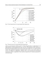
Criterion 3 hypothesis are clearly satisfied:

2
2
H
q
x
< 0


and
2
2
0
L
q
x



for some x (Fig. 6). Thus,
the maximum efficiency η
max
is given by the equation (54):

2
me
1
2
μ
me
1

x
x
1 - = 1 -
μ
(55)
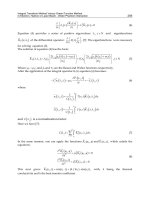
In solving, x
me
= μ and η
max
= 1 - μ

which corresponds to the Carnot efficiency; the other root,
x
me
= 0, is ignored. And the work is null for x
me
= μ; as a consequence the added heat is also
null (Fig. 6). Now regeneration conditions for the non-isentropic cycle will be established.
Again C
W
T
H
= mc
p
T
3
, T
H
= T
3

and T
L
= T
1
(cycle 1-2-3-4 in Fig. 3) and T
2

and T
4

are given by
the equations (42). Thus, using equations (42) and the structure of the work in the equation
(51), the work w

and the heat q
H

are:




*
1
2
H
2
11
w = η 1 - x - - 1 μ ;
η x

(1 - x)
q = 1 - 1 + μ*
η x









(56)
Maximizing,







**
2
*
4s 2s NI NI
***
2
Iη 1 - μ + Iμ - 1
T = IT ; x = Iμ and η = 1 -
IIη 1 - μ + μ Iμ - 1

(57)

Heat Analysis and Thermodynamic Effects

202

Fig. 6. Heat and work qualitative behavior for μ=0.25
.
where I = 1/η
1
η
2
and η
NI
is the efficiency to maximum work of the non-isentropic cycle.
Furthermore, the hypotheses from the Criterion 3 are fulfilled (the qualitative behavior of w

and q
H
is preserved, Fig. 6). In solving the resulting cubic equation, the maximum efficiency,
its extreme value and the inequality that satisfies are obtained:

   

   


2
11 2 21
2

max
122
11 2 21
me
122
me mw
ημ + ημ1 - μ (1 - ημ + η 1 - η
η
η = 1 -
μη μ 1 - η + η
ημ + ημ1 - μ 1 - ημ + η 1 - η
x=
ημ1 - η + η
Iμ xx





(58)
Now, following (Zhang et al., 2006), in a Brayton cycle a regenerator is used only when the
temperature of the exhaust working substance, leaving the turbine, is higher than the exit
temperature in the compressor (T
4
> T
2
). Otherwise, heat will flow in the reverse direction
decreasing the efficiency of the cycle. This point can be directly seen when T
4
< T

2
, because
the regenerative rate is smaller than zero and consequently the regenerator does not have a
positive role. From equations (42) the following relation is obtained:




43 1 1 2
2
11
T = T 1 - η 1 - x > T 1 + - 1 = T
η x






(59)
which corresponds to a temperature criterion which is equivalent to the first inequality of:


11
2
11
min
ηη
-β + β +4Iμ
x > x = ; β = - 1 + I - μ > 0

2
(60)
Indeed, from the equation (59):


2
2
min
x + βx - Iμ > 0
-β + β + 4Iμ
x > x = > 0
2
(61)

On the Optimal Allocation of the Heat Eexchangers of Irreversible Power Cycles

203
the inequality is fulfilled since
2
β + 4Iμ > β
. The other root is clearly ignored. Therefore, if
x
≤ x
min
, a regenerator cannot be used. Thus, the first inequality of (60) is fulfilled.
Criterion 3. If the cycle operates either to maximum work or efficiency, a counterflow heat
exchanger (regenerator) between the turbine and compressor outlet is a good option to
improve the cycle. For other operating regimes is enough that the inequality (61) be fulfilled.
When the operating regime is at maximum efficiency the inequality of (61) is fulfilled.
Indeed,

   


   







me min
2
1221
me min 1
122
2
2
2
1221
122
22 2
12 2
x > x
ημ1 - μ (1 - ημ + η 1 - η
β + 4Iμ
x- x = ημ + β + -
2 ημ1 - η + η
ημ1 - μ (1 - ημ + η 1 - η

β + 4Iμ
- =
2 ημ1 - η + η
ηη1 - μ + μβη1 - μ + μ + 4Iμ +














   


2
2
1221
122
4ημ1 - μ >0
ημ1 - μ (1 - ημ+η 1 - η
β +4Iμ
>
2 ημ1 - η +η

(62)
where the following elementary inequality has been applied: If a, b > 0, then a < b
⇔ a
2
< b
2
.
If the operating regime is at maximum work, the proof is completely similar to the equations
(62). An example of a non-isentropic regenerative cycle is provided in (Aragón-González et
al., 2010).
3.2. Optimal analytical expressions
If the total number of transfer units of both heat exchangers is N, then, the following
parameterization of the total inventory of heat transfer (Bejan, 1988) can be included in the
equation (50):



HL H L
N + N = N; N =
y
N and N = 1 -
y
N
(63)
For any heat exchanger

UA
C
N , where U is the overall heat-transfer coefficient, A the heat-
transfer surface and C the thermal capacity. The number of transfer units in the hot-side and

cold-side, N
H

and N
L
, are indicative of both heat exchangers sizes. And their respective
effectiveness is given by (equation (9)):




-1 - yN
-yN
HL
ε = 1 - e ; ε = 1 - e
(64)
Then, the work w (equation (50)) depends only upon the characteristics parameters x and y.
Applying the extreme conditions:
w
x
= 0


;
w
y
= 0


, the following coupled optimal analytical

expressions for x and y, are obtained:





 
1
NE
1
NE
z- z Cz - B
x = μ;
z - 1 Az - Bz
11 Ax - Bμ
y = + ln
22N Bx - Cμ



(65)

Heat Analysis and Thermodynamic Effects

204
where z
1
= e
N
; z = e

yN
; A = η
1
η
2
e
N
+ 1 - η
2
; B = e
N
(η
1
η
2
+ 1 - η
2
)

and C=e
N
-η
2
+ η
1
η
2
.
The equations (65) for x
NE

and y
NE
cannot be uncoupled. A qualitative analysis and its
asymptotic behavior of the coupled analytical expressions for x
NE
and y
NE
(equations (65))
have been performed (Aragón-González (2005)) in order to establish the bounds for x
NE
and
y
NE
and to see their behaviour in the limit cases. Thus the following bounds for x
NE
and y
NE

were found:


1
2
NI NE NE
0 < x x < 1; 0 <
y
< 
(66)
where x
NI

is given by the equation (57). The inequality (66) is satisfied because of
 


1
1
z-z Cz- B
z - 1 Az - Bz
1 < I 
. If I = 1 (η
1
= η
2
= 100%), the following values are obtained: x
NE
= x
CNCA
=
 ; y
NE
= y
E
= ½ which corresponds to the endoreversible cycle. In this case necessarily:

ε
H
=
ε
L
= 1. Thus, the equations (65) are one generalization of the endoreversible case [η

1
= η
2
= 1, 0 <
ε
H
, ε
L
< 1]. The optimal allocation (size) of the heat exchangers has the following asymptotic
behavior:
12
NE
N
lim
y
= ;

12
12
NE
η ,η 1
lim y =

. Also, x
NE

has the following asymptotic behavior:

NE NI
N

lim x = x ;

NE NI
N
lim η = η

. Thus, the non-isentropic [ε
H
= ε
L
= 1, 0 < η
1
,

η
2
< 1] and
endoreversible [η
1
= η
2
= 1, 0 < ε
H
, ε
L
< 1] cycles are particular cases of the cycle herein
presented. A relevant conclusion is that the allocation always is unbalanced (y
NE
< ½).
Combining the equations (65), the following equation as function only of z, is obtained:

 
 
2
1
1
2
11
z - z Cz - B
Bz - Cz
μ =
Az - z B z - 1 Az - Bz



(67)
which gives a polynomial of degree 6 which cannot be solved in closed form. The variable
z
relates (in exponential form) to the allocation (unbalanced, ε
H
< ε
L
) and the total number of
transfer units N

of both heat exchangers. To obtain a closed form for the effectiveness ε
H
, ε
L
,

the equation (67) can be approximated by:

2
1
2
1
Bz - Cz 1 1
μ = + H
Az - z B 2 2






(68)
with
 
 
1
1
z- z Cz - B
z - 1 Az - Bz
H = ; and using the linear approximation:

 


1
2

2
H=1 + H-1 +O H-1
.
It is remarkable that the non-isentropic and endoreversible limit cases are not affected by the
approximation and remain invariant within the framework of the model herein presented.
Thus, this approximation maintains and combines the optimal operation conditions of these
limit cases and, moreover, they are extended. The equation (68) is a polynomial of degree 4
and it can be solved in closed form for z

with respect to parameters: μ or N, for realistic
values for the isentropic efficiencies (Bejan (1996)) of turbine and compressor:

η
1
= η
2
= 0.8 or
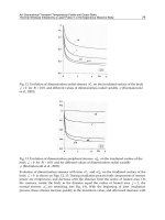
0.9, but it is too large to be included here. Fig. 7 shows the values of z (z
mp
) with respect to μ.
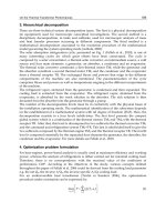
Using the same numerical values, Fig. 8 shows that the efficiency to maximum work η
NE
,
with respect to μ, can be well approached by the efficiency of the non-isentropic cycle η
NI

(equation (57)) for a realistic value of N = 3 and isentropic efficiencies of 90%. The behavior
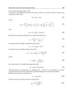
of y
NE
with respect to the total number of transfer units N of both heat exchangers, with the

same numerical values for the isentropic efficiencies of turbine and compressor and μ = 0.3, are

On the Optimal Allocation of the Heat Eexchangers of Irreversible Power Cycles

205
presented in Fig. 9. When the number of heat transfer units, N, is between 2 to 5, the
allocation for the heat exchangers y
NE
is approximately 2 - 8% or 1 - 3%, less than its
asymptotic value or ½, respectively.


Fig. 7. Behaviour of
z(z
mp
) versus μ, if η
1
= η
2
=0.8 and N=3.


Fig. 8. Behaviour of η
NE
, η
NI
and η
CNCA
versus μ, if η
1

= η
2
=0.8 or 0.9 and N=3.


Fig. 9. Behavior of y
NE
versus N, when η
1
= η
2
=0.8 or 0.9 and μ=0.3.
This result shows that the size of the heat exchanger in the hot side decreases. Now, if the
Carnot efficiency is 70% the efficiency η
NE
is approximately 25 - 30% or 10 - 15%, when the

Heat Analysis and Thermodynamic Effects

206
number of heat transfer units N is between 2 and 5 and the isentropic efficiencies are
η
1
= η
2
= 0.9 or 0.8 respectively, as is shown in Fig. 9.
Now, if η
1
= η
2

= 0.8 (I = 1.5625) ; y
NE
= 0.45 then
N3.5

(see Fig. 9) and for the equations
(64): ε
H
= 0.74076 and ε
L
= 0.80795. Thus, one cannot assume that the effectiveness are the
same: ε
H
= ε
L
< 1 ; whilst I > 1. Current literature on the Brayton-like cycles, that have taken
the same less than one effectiveness and with internal irreversibilities, should be reviewed.
To conclude, ε
H
= ε
L
if and only if the allocation is balanced (y = ½) and the unique
thermodynamic possibility is: optimal allocation balanced (y
NE
= y
E
= ½); that is ε
H
= ε
L

. And
ε
H
<ε
L
if and only if I>1 there is internal irreversibilities.
4. Conclusions
Relevant information about the optimal allocation of the heat exchangers in power cycles
has been described in this work. For both Carnot-like and Brayton cycles, this allocation is
unbalanced. The expressions for the Carnot model herein presented are given by the
Criterion 1 which is a strong contribution to the problem (following the spirit of Carnot’s
work): to seek invariant optimal relations for different operation regimes of Carnot-like
models, independently from the heat transfer law. The equations (26)-(28) have the above
characteristics. Nevertheless, the optimal isentropic temperatures ratio depends of the heat
transfer law and of the operation regime of the engine as was shown in the subsection 2.2
(Fig. 5). Moreover, the equations (26) can be satisfied for other objective functions and other
characteristic parameter: For instance, algebraic combination of power and/or efficiency
and costs per unit heat transfer; as long as these objective functions and parameters have
thermodynamic sense. Of course, the objective function must satisfy similar conditions to
the equations (20) and (21). But this was not covered by this chapter's scope.

The study performed for the Brayton model combined and extended the optimal operation
conditions of endoreversible and non-isentropic cycles since this model provides more
realistic values for efficiency to maximum work and optimal allocation (size) for the heat
exchangers than the values corresponding to the non-isentropic or the endoreversible
operations. A relevant conclusion is that the allocation always is unbalanced (y
NE
< ½).
Furthermore, the following correlation can be applied between the effectiveness of the
exchanger heat of the hot and cold sides:

NE
1
z
HL
-N
NE
1 -
ε = ε
1 - z e
(69)
where z
NE
is calculated by the equation (68) and shown in Fig. 7, which can be used in the
current literature on the Brayton-like cycles. In subsection 3.1 the problem of when to fit a
regenerator in a non-isentropic Brayton cycle was presented and criterion 3 was established.
On the other hand, the qualitative and asymptotic analysis proposed showed that the non-
isentropic and endoreversible Brayton cycles are limit cases of the model of irreversible
Brayton cycle presented which leads to maintain the performance conditions of these limit
cases according to their asymptotic behavior. Therefore, the non-isentropic and
endoreversible Brayton cycles were not affected by our analytical approximation and
remained invariant within the framework of the model herein presented. Moreover, the
optimal analytical expressions for the optimal isentropic temperatures ratio, optimal
allocation (size) for the heat exchangers, efficiency to maximum work and maximum work
obtained can be more useful than those we found in the existing literature.

On the Optimal Allocation of the Heat Eexchangers of Irreversible Power Cycles

207
Finally, further work could comprise the analysis of the allocation of heat exchangers for a

combined (Brayton and Carnot) cycle with the characteristics and integrating the
methodologies herein presented.
5. References
Andresen, B. & Gordon J. M. Optimal heating and cooling strategies for heat exchanger
design. J. Appl. Phys
. 71, (January 1992) pp. 76-79, ISSN: 0021 8979.
Aragón-González G., Canales-Palma A. & León-Galicia A. (2000). Maximum irreversible
work and efficiency in power cycles.
J. Phys. D: Appl. Phys. Vol. 33, (October 2000)
pp. 1403-1410, ISSN:
1361-6463.
Aragón-González G., Canales-Palma A., León-Galicia A. & Musharrafie-Martínez, M. (2003)
A criterion to maximize the irreversible efficiency in heat engines,.
J. Phys. D: Appl.
Phys. Vol. 36, (Janaury 2003) pp. 280-287, ISSN: 1361-6463.
Aragón-González G., Canales-Palma A., León-Galicia A. & Musharrafie-Martínez, M. (2005).
The fundamental optimal relations and the bounds of the allocation of heat
exchangers and efficiency for a non-endoreversible Brayton cycle.
Rev. Mex. Fis.
Vol. 51 No. 1, (January 2005), pp. 32-37, ISSN: 0035–00IX.
Aragón-González G., Canales-Palma A., León-Galicia A. & Morales-Gómez, J. R. (2006).
Optimization of an irreversible Carnot engine in finite time and finite size, Rev.
Mex. Fis. Vol. 52 No. 4, (April 2006), pp. 309-314, ISSN: 0035–00IX.
Aragón-González G., Canales-Palma A., León-Galicia A. & Morales-Gómez, J. R. (2008).
Maximum Power, Ecological Function and Eficiency of an Irreversible Carnot
Cycle. A Cost and Effectiveness Optimization.
Braz. J. of Phys. Vol. 38 No. 4, (April
2008), pp. 543-550, ISSN: 0103-9733.
Aragón-González G., Canales-Palma A., León-Galicia A. & Rivera-Camacho, J. M. (2009).
The fundamental optimal relations of the al location, cost and effectiveness of the

heat exchangers of a Carnot-like power plant.
Journal of Physics A: Mathematical and
Theoretical. Vol. 42, No. 42, (September 2009), pp. 1-13 (425205), ISSN: 1751-8113.
Aragón-González G., Canales-Palma A., León-Galicia A. & Morales-Gómez, J. R. (2010). A
regenerator can fit into an internally irreversible Brayton cycle when operating in
maximum work.
Memorias del V Congreso Internacional de Ingeniería Física, ISBN:
978-607-477-279-1, México D.F., May 2010.
Arias-Hernández, L. A., Ares de Parga, G. and Angulo-Brown, F. (2003). On Some
Nonendoreversible Engine Models with Nonlinear Heat Transfer Laws.
Open Sys.
& Information Dyn. Vol. 10, (March 2003), pp. 351-75, ISSN: 1230-1612.
Bejan, A. (1988). Theory of heat transfer-irreversible power plants.
Int. J. Heat Mass Transfer.
Vol. 31, (October 1988), pp. 1211-1219, ISSN: 0017-9310.
Bejan, A. (1995) Theory of heat transfer-irreversible power plants II. The optimal allocation
of heat exchange equipment
. Int. J. Heat Mass Transfer. Vol. 38 No. 3, (February
1995), pp. 433-44, ISSN:
0017-9310.
Bejan, A. (1996). Entropy generation minimization, CRC Press, ISBN 978-0849396519, Boca
Raton, Fl.
Chen, J. (1994). The maximum power output and maximum efficiency of an irreversible
Carnot heat engine
. J. Phys. D: Appl. Phys. Vol. 27, (November 1994), pp. 1144-1149,
ISSN: 1361-6463.
Chen L., Cheng J., Sun F., Sun F. & Wu, C. (2001). Optimum distribution of heat exchangers
inventory for power density optimization of an endoreversible closed Brayton
cycle.
J. Phys. D: Appl Phys. Vol. 34, (Janaury 2010), pp. 422-427, ISSN 1361-6463.

Heat Analysis and Thermodynamic Effects

208
Chen, L., Song, H., Sun, F. (2010). Endoreversible radiative heat engine configuration for
maximum efficiency.
Appl. Math. Modelling, Vol. 34 (August 2010), pp. 1710–1720,
ISSN: 0307-904X.
Durmayaz, A. Sogut, O. S., Sahin, B. and Yavuz, H. (2004). Optimization of thermal systems
based on finite time thermodynamics and thermoeconomics
. Progr. Energ. and
Combus. Sci.
Vol. 30, (January 2004), pp. 175-217, ISSN: 0360-1285.
Herrera, C. A., Sandoval J. A. & Rosillo, M. E. (2006). Power and entropy generation of an
extended irreversible Brayton cycle: optimal parameters and performance. J
. Phys.
D: Appl. Phys.
Vol. 39. (July 2006) pp. 3414-3424, ISSN: 1361-6463.
Hoffman, K. H.,. Burzler, J. M and Shuberth, S. (1997). Endoreversible Thermodynamics.
J.
Non-Equilib. Thermodyn.
Vol. 22 No. 4, (April 1997), pp. 311-55, ISSN: 1437-4358.
Kays, W. M. & London, A. L. (1998).
Compact heat exchangers (Third edition), McGraw-Hill,
ISBN: 9780070334182, New York.
Leff, H. S.(1987). Thermal efficiency at maximum work output: New results for old engines.
Am J. Phys. Vol. 55(February 1987), pp. 602-610, ISSN: 0894-9115.
Lewins, J. D. (2000). The endo-reversible thermal engine: a cost and effectiveness optimization.
Int. J. Mech. Engr. Educ., Vol. 28, No. 1, (January 2000), pp. 41-46, ISSN: 0306-4190
Lewins, J. D. (2005). A unified approach to reheat in gas and steam turbine cycles.

Proc. Inst.
Mech. Engr. Part C
: J. Mechanical Engineering Science. Vol. 219, No 2 (November
2000), (March 2005), pp. 539-552
., ISSN: 0263-7154.
Lienhard
IV, J. H. & Lienhard V, J. H. (2011) A Heat Transfer Textbook (Fourth edition),
Phlogiston Press, ISBN: 0-486-47931-5, Cambridge, Massachusetts
Nusselt, W. Eine Neue Formel für den Wärmedurchgang im Kreuzstrom.
Tech. Mech.
Thermo-Dynam
. Vol. 1, No. 12, (December 1930), pp. 417–422.
Sanchez Salas, N., Velasco, S. and Calvo Hernández, A. (2002). Unified working regime of
irreversible Carnot-like heat engines with nonlinear heat transfer laws.
Energ.
Convers. Manage.
Vol. 43 (September 2002), pp. 2341—48, ISSN: 0196-8904.
Sontagg, R. E., Borgnankke, C. & Van Wylen, G. J. (2003), Fundamentals Of Thermodynamics
(Sixth edition), John Wyley and Sons, Inc., ISBN: 0-471-15232-3, New York
Swanson L. W (1991). Thermodynamic optimization of irreversible power cycles wit
constant external reservoir temperatures.
ASME J. of Eng. for Gas Turbines Power
Vol. 113 No. 4, (May 1991), pp. 505-510, ISSN: 0742-4795.
Ust Y., Sahin B. and Kodal A. (2005). Ecological coefficient of performance (ECOP)
optimization for generalized irreversible Carnot heat engines.
J. of the Energ. Inst.
Vol. 78 No. 3 (January 2005), 145-151, ISSN: 1743-9671
.
Wang L.G., Chen L., F. R. Sun & Wu, C. (2008). Performance optimisation of open cycle
intercooled gas turbine power with pressure drop irreversibilities.

J. of the Energ.
Inst.
Vol. 81 No. 1, (January 2008), pp. 31-37, ISSN: 1743-9671.
Wu C. & Kiang R. L. (1991). Power performance of a non-isentropic Brayton cycle.
ASME J. of
Eng. for Gas Turbines Power
Vol. 113 No.4, (April 1991), pp. 501-504, ISSN: 0742-4795.
Yan Z. and L. Chen . The fundamental optimal relation and the bounds of power output and
efficiency for and irreversible Carnot engine. J. Phys. A: Math. Gen. Vol. 28,
(December 1995) pp. 6167-75, ISSN: 1751-8113.
Yilmaz T. (2006). A new performance criterion for heat engines:efficient power.
J. Energy
Inst., Vol. 79, (January 2006), pp. 38—41, ISSN: 1743-9671.
Zhang, Y., Ou, C., Lin, B., and Chen, J. (2006). The Regenerative Criteria of an Irreversible
Brayton Heat Engine and its General Optimum Performance Characteristics.
J.
Energy Resour. Technol.
Vol, 128 No. 3, (2006), pp. 216-222, ISSN: 0195-0738.
Part 3
Gas Flow and Oxidation

10
Gas-Solid Flow Applications for Powder
Handling in Industrial Furnaces Operations
Paulo Douglas Santos de Vasconcelos¹
and André Luiz Amarante Mesquita²
¹Albras Alumínio Brasileiro S/A
²Federal University of Pará
Brazil
1. Introduction

Gas-solid flow occurs in many industrial furnaces operations. The majority of chemical
engineering units operations, such as drying, separation, adsorption, pneumatic conveying,
fluidization and filtration involve gas-solid flow.
Poor powder handling in an industrial furnace operation may result in a bad furnace
performance, causing errors in the mass balance, erosion caused by particles impacts in the
pipelines, attrition and elutriation of fines overloading the bag houses. The lack of a good
gas-solid flow rate measurement can cause economic and environmental problem due to
airborne.
The chapter is focused on the applications of powder handling related with furnaces of the
aluminum smelters processes such as anode baking furnace and electrolytic furnace (cell) to
produce primary aluminum.
The anode baking furnace illustrated in figure 1 is composed by sections made up of six cells
separated by partitions flue walls through which the furnace is fired to bake the anodes. The
cell is about four meters deep and accommodates four layers of three anode blocks, around
which petroleum coke is packed to avoid air oxidation and facilitate the heat transfer.
During the baking process, the gases released are exhausted to the fume treatment center



(a) (b)
Fig. 1. a) Anode baking furnace building overview; b) Petroleum coke being unpacked from
anode coverage by vacuum suction.

Heat Analysis and Thermodynamic Effects

212
(FTC) where the gases are adsorbed in a dilute pneumatic conveyor and in an alumina
fluidized bed. The handling of alumina is made via a dense phase conveyor.
The baked anode is the positive pole of the electrolytic furnace (cell) which uses 18 of them
by cell. The pot room and the overhead multipurpose crane are illustrated in figure 2.

(a) (b)
Fig. 2. a) Aluminum smelter pot room, b) Overhead crane being fed of alumina from a day
bin by a standard air slide.


(a) (b)
Fig. 3. a) Electrolytic furnace being fed of alumina by the overhead crane; b) Sketch of
electrolytic furnace being continuous fed of alumina by a special fluidized pipeline.
The old aluminum smelters feed their electrolytic cells with the overhead cranes as can be
seen in figures 2 and 3. This task is very hard to the operators and causes spillage of alumina
to the pot room workplace. This nuisance problem is being solved by the development of a
special multi-outlets nonmetallic fluidized pipeline.
The fundamentals of powder pneumatic conveying and fluidization will be discussed in this
chapter, such as the definition of a pneumatic conveying in dilute and dense phase, the
fluidized bed regime map as illustrated in figure 5 and finally the air fluidized conveyor.
Firstly, petro coke and alumina used as raw materials in the primary aluminum process is
characterized using sieve analyses (granulometry size distribution). Then, bulk and real
density are determined in the laboratory analyses; with these powder physical properties,
they can be classified in four types using the Geldart’s diagram as illustrated in figure 4.

Gas-Solid Flow Applications for Powder Handling in Industrial Furnaces Operations


213

Fig. 4. Powder classification diagram for fluidization by air – source: (Geldart, 1972).
The majority of powders used in the aluminum smelters belong to groups A and B
considering Geldart’s criteria.

Fig. 5. Flow regime map for various powders.
This figure 5 summarized the fluidized bed hydrodynamics related with powders classified
according to Geldart’s criteria.
Once the velocities associated with each mode of operation are determined, the pressure
drop of the regime is calculated so that the gas-solid flow is predicted using the modeling
and software adequated to optimize the industrial installation.
The pipeline and air fluidized conveyors feeding devices are also discussed in this chapter.
Finally two cases studies applied in the baking furnace of pneumatic powder conveying in
dilute phase are shown as a result of a master degree dissertation. Another case study is the
development of an equation to predict the mass solid flow rate of the air-fluidized conveyor
as a result of thesis of doctorate. The equation has design proposal and it was used in the
design of a fluidized bed to treat the gases from the bake furnace and to continuously
alumina pot feeding the electrolyte furnaces to produce primary aluminum.

Heat Analysis and Thermodynamic Effects

214
2. Fundamentals of pneumatic conveying of solids
Pneumatic conveying of solids is an engineering unit operation that involves the movement
of millions of particles suspend by draft in dilute phase or in a block of bulk solids in dense
phase inside a pipeline. Figure 6 illustrates a pneumatic conveying of solids with the
essential components, like the air mover, feeding device, pipeline and bag house.


Fig. 6. Typical pneumatic conveyor layout – source: (Klinzing et al, 1997).
A good criterion showed in table 1 to decide if the transport of solids in air will be in dilute
phase or in dense phase is the mass load ratio (


) calculated by the equation 1.


g
Gv


 (1)
Where
.
G ,
.
v and
g

are the solid mass flow rate, gas (air) volume flow rate and gas (air)
density.

Mode of transport of solids

Solids –to – air ratio (

)

Dilute phase 0 - 15
Dense phase > 15
Table 1. Systems’ classification concerning solids-to-air ratio - source: (Klinzing et al, 1997).
Figure 7 illustrates a variety of solids modes of transportation and the states diagrams
showing the log of the pipeline pressure drop versus the log of the air velocity inside the
pipeline. From figure 7 it is concluded that in dilute phase the pneumatic conveyor has high

air velocity, low mass load ratio, and low pressure drop in the pipeline. In dense phase
mode the conveyor operates with high mass load rate, low air velocity but high pressure

Gas-Solid Flow Applications for Powder Handling in Industrial Furnaces Operations


215
drop in the pipeline. The engineer responsible for the project has to analyze which is the best
solution for each case study.


Fig. 7. Conveying conditions showing the changes in solids loading; left: State diagram
horizontal flow, right: State diagram vertical flow - source: (Klinzing et al, 1997).
2.1 Pressure drop calculation in the pipeline
The equations given here are based on the hypothesis that the gas-solid flow is in dilute
phase. Some assumptions such as: transients in the flow (Basset forces) are not considered
nor the pressure gradient around the particles (this is considered negligible in relation to the
drag, gravitational and friction forces).
The pressure drop due to particle acceleration is not considered.
The flow is considering incompressible, omnidimensional and the concentration of solids
particles is uniform. The physical properties of the two phases are temperature dependent.
The mass flow rate for each phase can be expressed by the following equations:

.
gg
mc mc
mVA


(2)

.
sss
GVA


 (3)
Where the suffixes g and s denote gas and solid, respectively,
mc
V is the minimum air
velocity in dilute phase in relation to the pipe cross section A,
s

and
mc

are the volume
fraction occupied by the solid and gas inside the pipeline as follows:

.
2
4
s
s
ss
A
G
A
DV




(4)
D is the pipe diameter and
s
V
is the particle velocity. The void or porosity at the minimum
air velocity
mc

, in other words is the fraction of volume occupied by the gas (air).

1
g
mc s
A
A



 (5)
Lo
g

(
avera
g
e air velocit
y)

Lo
g

(
avera
g
e air velocit
y)


Heat Analysis and Thermodynamic Effects

216
Velocity of the particle
s
V and the particle terminal velocity
t
V calculation:
In this chapter it is considered the models of (Yang, 1978) for the pressure drop calculation.

2
4.7
2
1
ss
mc
st mc
mc
fV
V

VV
gD


 
(6)



2
18
p
s
g
t
g
gd
V





, 3.3K

(7)



0.71

0.71 1.14
0.29 0.43
0.153
psg
t
gg
gd
V



 , 3.3 43.6K


(8)



12
1.74
ps g
t
g
gd
V













, 43.6 2360K


(9)

K is a factor that determines the range of validation for the drag coefficient expressions,
when the particle Reynolds number is unknown, and given by:


13
2
gs g
p
g
g
Kd
 












(10)
Where
g

is the gas dynamic viscosity, g acceleration due gravity,
g

gas (air) density,
p
d
the particle diameter,
s
f
is the solid friction factor.
The total pressure drop,
T
P

for gas-solid flow is calculated with the contribution of the
static pressure
E
P
, and friction loss
F
P


for both phases:
()()
TEFsEF
g
PPP PP

    (11)



Ess
s
PL
g

 (12)



Egg
g
PL
g

 (13)
The contribution due to the friction factor given by the Darcy equation:


2

2
ssp
F
s
f
VL
P
D


(14)


2
2
ggg
F
g
f
VL
P
D

 (15)
Where,
s
f
and
g
f

are the friction factor for the solid and gas (air), respectively. The friction
factor for the gas is calculated by the Colebrook equation.

Gas-Solid Flow Applications for Powder Handling in Industrial Furnaces Operations


217

1 18.7
1.74 2log 2
4Re4
gg
ff





 




(16)

R
gmc
e
g
VD



 (17)
e
R is the Reynolds number,

is the relative roughness of the pipe, this equation is implicit
for
g
f
. The friction factors due to solids in vertical and horizontal flow are obtained by the
model of (Yang, 1978).

0.979
3
1(1)
0.00315
mc mc t
sv
mc
mc
s
mc
V
f
V
V














(18)


1.15
3
1
1
0.0293
g
mc
mc mc
sh
mc
V
f
gD














(19)
3. Fundamentals of powder fluidization
Fluidization is an engineering unit operation that occurs when a fluid (liquid or gas) ascend
trough a bed of particles, and that particles get a velocity of minimum fluidization
m
f
V enough to suspend the particles, but without carry them in the ascending flow. Since
this moment the powder behaves like a liquid at boiling point, that is the reason for term
“fluidization”. Figure 8 gives a good understanding of the minimum fluidization velocity.


Fig. 8. Fixed and a fluidized bed of particles at a minimum fluidization velocity - adapted
from (Kunii & Levenspiel, 1991).

Heat Analysis and Thermodynamic Effects

218
3.1 Minimum fluidization velocity calculation
In this chapter it will be point out the beginning (fluidized beds) and the ending (pneumatic
transport) of the flow regime map illustrated in figure 5.
The minimum fluidization velocity will be calculated by the (Ergun, 1952) equation 20 and

it‘s experimental value obtained using a permeameter as showed in figure 19.


Fig. 9. Pressure drop through a bed of particles versus superficial air velocity – source:
(Mills, 1990).

32
2
32 3
(1 ) (1 )
(1 )( ) 150 1.75
()
mf g mf mf g mf
m
f
s
g
m
f
m
f
sp
mf s p mf
VV
gAVBV
d
d
 



 

   (20)
Calculating C by equation 21 we get an equation of second power, which the positive
solution is calculated by equation 22.
(1 )( )
mf s g
Cg



 (21)

2
4
2
mf
AA BC
V
B
 

(22)
Where
A and B are the viscous and the inertial factors of the Ergun equation, C is the
weight per unit volume of the bed of particles.
Fluidization is related with small velocities, the factor B is negligible and the Ergun equation
can be simplified with an error less than 1% by the equation 23.

32

()()
150(1 )
sg mfsp
mf mf
mf g
gd
C
VV
A
 


 

(23)

Gas-Solid Flow Applications for Powder Handling in Industrial Furnaces Operations


219
For an incipient fluidization, when the weight of particles equals the drag force, it is a good
attempt to consider the porosity at the minimum fluidization velocity
m
f

equals the
porosity

of the fixed bed. The porosity of the fixed bed is calculated by the equation 24.

1
bnv
s



 (24)

s
bnv
total
M
V

 (25)
Where
bnv

is the non-vibrated bulk density,
s

is the solid real density calculated in a
laboratory by a pycnometer,
s
M
is the total mass of particles weighted in a electronic scale,
total
V is the total volume of particles and voids in the sample previously weighted in a
electronic scale,
p

d
is the particle mean diameter obtained by sieve analysis in a laboratory,
s

is the particle sphericity, that can be estimated by equation 26 with
p
d in (m).

1
0.255 ( ) 1.85
p
s
Log d



 (26)
Other important velocity in pneumatic transport and fluidization is the particle terminal
velocity
t
V that is calculated by equations 7 to 10.
4. Air-fluidized conveyors
4.1 Pile powder flow - simple model
Assuming that the block of alumina is made of non-cohesive material with uniform
porosity

, and is inclined at the moment of analysis in an angle

to the horizontal plane,
this elemental block has a constant width

z

.
Also assuming that the flow is isothermal in the (y) direction, a simple force balance requires
that:
Gravitational force component = Drag force + Frictional force due to apparent viscosity (27)

.(1 ) ( ) ( ) ( )
s
gsen xyz P xz yz

 

     (28)


Fig. 10. Force balance acting on an elemental pecked bed block of alumina flowing to repose.


Heat Analysis and Thermodynamic Effects

220
Assuming that the particles of the block are ready to slip over each other, the internal
friction between the particles is obtained from equation 29 – source: (Schulze, 2007).
tan .
x
y
ix




(29)
Assuming that the cohesion between particles is negligible,
x
y

is the shear stress in the
plane parallel to the plane (y-z),
i

is the angle of internal friction of the powder, and
x


the normal stress in the direction (x) is:

(1 ) cos ( )
s
x
g
x
y
z
yz
 






(30)
Rearranging the equations 28 to 30 is obtained the pressure drop
P

of flow in the (y)
direction by the equation 31.

(1 ) ( tan cos )
si
P
g sen
y



 

(31)
The pile of alumina powder reaches the equilibrium between gravity force and Interparticles
forces with an angle of repose

, so in this moment the angle alpha of pile turns beta
(


 ).
The friction coefficient between the particles of the pile is the tangent of the particles internal
friction angle, given by equation 32.

tan

i



(32)
4.2 Engineering model for design proposal to air fluidized conveyors
The proposed model for gas-solid flow is based in the figure 11 and is fitted by the following
considerations:
1.
The height of the moving fluidized bed in the (y) and (z) directions is constant;
2.
The flow of the fluidizing air and that of moving fluidized bed are both steady and full
developed in the mean flow;
3.
The flow of the moving fluidized bed is in the (y) direction;
4.
The slip velocity between the particles and the air in the (y) direction will be negligible;
5.
The direction of the fluidizing air will have components in the (x) and (y) directions
both in the inlet and outlet of the moving fluidized bed;
6.
The pressure of fluidization is constant for every conveyor inclination;
7.
The gas-solid flow is considered isothermal and irrotacional;
8.
It will not be considered the mass and heat transfer between the particles and the air;
9.
The shear stress
x
y


of particles will vary in the (x) direction and will be maximum in
the bottom and minimum in the top of the elemental block of alumina;
10.
The electrostatic and van der Walls forces in the proposed model it will not be
considered;
11.
The porosity of the moving fluidized bed varies with the fluidizing air velocity but will
be considered isotropic;
12.
The shear stress of the particles is a function of the moving fluidized bed porosity;

Gas-Solid Flow Applications for Powder Handling in Industrial Furnaces Operations


221



Fig. 11. (a) Elemental block of alumina in an air-fluidized conveyor inclined of an angle

,
(b) in the left: elemental block alumina being fluidized by the components of superficial air
velocity V, in the right: balance of forces per unit of volume acting on the elemental block of
alumina.
13.
The moving fluidized bed has a rheological behavior similar to a liquid;
14.
The stress in the side walls of the air fluidized conveyor is considered negligible due to
air lubrication,

15.
The friction coefficient between particles and the fluidizing felt in the bottom will be
minimized by the fluidizing air velocity, and will follow the model of (Kozin &
Baskakov, 1996) for angle of repose in the fluidized state, but adjusted with k factor;
16.
There will not be rate of mass accumulation inside the air fluidized conveyor see
equation 33;
17.
It will not have rate of momentum accumulation inside of the air fluidized conveyor see
equation 12;
18.
The drag force of the particles inside the moving fluidized bed will follow the Ergun
(1952) equation.

Heat Analysis and Thermodynamic Effects

222
19. The elemental block of alumina will be considered continuum;
20.
The maximum solid mass flow rate will be determined by the model proposed by
(Jones, 1965) for powder discharge from small silos – powder liquid-like behavior;
21.
For a full opened gate valve of the feed bin the mass flow rate of the assemble bin-air
fluidized conveyor will follow the rhythm of the air fluidized conveyor;
22.
The model will not consider the contribution of the height of the bulk solids H in the
feeding bin.
4.2.1 Equation of continuity
It was assumed in the above considerations that there will not be rate of mass accumulation
inside the air fluidized conveyor according to equation 33.

Rate of mass Rate of mass Rate of mass
0
accumulation in out





(33)
Equation 33 points out that the mass of gas and solid mixture entering the air fluidized
conveyor must be the same as in the outlet of the air fluidized conveyor during the full-
developed steady flow regime. So, for the two phases of the flow we have.
Gas phase:

0
lf g x lf g y
VV
xy
 




(34)
Where:
x
V and
y
V

are the component of the superficial air velocity in the (x) and (y)
directions,
g

is the gas or air density,
l
f

is the moving fluidized bed porosity.
Solid phase:

(1 ) 0
lf s s
V
y





(35)
Where:
s
V
is the velocity of the moving fluidized bed in the (y) direction as it was
supposed in the model considerations,
s

is the solid or particle density.
4.2.2 The momentum equation

Let’s consider the elemental block of alumina in figure 11 with porosity
l
f

flowing in a
fluid with constant density
g

and bulk density
b

of the mixture gas-solid and air
superficial velocities
x
V and
y
V in the (x) and (y) directions and the particles flowing in the
(y) direction without slipping the air in this direction with velocity
s
V .
As it was supposed there will not be rate of momentum accumulation inside of the air
fluidized conveyor according to equation 36.

Rate of Rate of Sum of forces
0
momentum in momentum out acting on s
y
stem
  
 

  
  
(36)
The equation 36 is in truth is a force balance equation; the terms used in this equation are as
follows:

Gas-Solid Flow Applications for Powder Handling in Industrial Furnaces Operations


223
Rate of momentum in across surface at (x) in the beginning of the elemental block
(Moment transport due to powder apparent viscosity);
()
xy
yzx



Rate of momentum in across surface at (x+ x

) in the end of the elemental block
(Moment transport due to powder apparent viscosity);
()
xy
yzx x

 
Rate of momentum in across surface at (y=0)
(Momentum due to gas-solid motion)
()()

yby
xzV V y



Rate of momentum in across surface at (y +
y

)
(Momentum due to gas-solid motion)
()()
yby
xzV V y y




Pressure force on the elemental block at (x) in the (x) direction
()P
y
zx

Pressure force on the elemental block at (x+
x

) in the(x) direction ()P
y
zx x 
Pressure force on the elemental block at (y=0) in the (y) direction
()Pxz

y

Pressure force on the elemental block at (y
+
y

) in the (y) direction
()Pxz
yy
 

Gravity force acting on the mixture gas-solid in the (x) direction
()cos
b
xyz g




Gravity force acting on the mixture gas-solid in the (y) direction
()
b
x y z gsen




Drag force acting on the mixture gas-solid in the (x) direction
Dx
F

Drag force acting on the mixture gas-solid in the y) direction
D
y
F
Friction force due to gravity and fluid during block motion in the(y) direction
f
riction
F

Substituting the terms relating with (x) direction in the moment balance equation 36 results:

()P
y
zx - ()P
y
zx x

-
Dx
F
+
()cos
b
xyz g



= 0 (37)
Equation 11 is now divided by the elemental volume
xyz


 and, if x

is allowed to be
infinitely small 0x , it is obtained:

cos
bDx
P
g
F
x





(38)
Where
_
Dx
F is the drag force per unit of volume of the elemental block in (x) direction.
Substituting the terms relating with (y) direction in the moment balance equation 10 results
equation 39:
()
xy
yzx

 - ()
xy

y
zx x


+ ()()
yby
xzV V y

 - ()()
yby
xzV V y y


+
+
()Pxz
y
 - ()Pxz
yy

+
()
b
x y z gsen



+
D
y

F -
f
riction
F = 0 (39)
Equation 37 is now divided by the elemental volume
xyz


and, if x

and
y

are allowed
to be infinitely small 0x

 and
0y


it is obtained:

0
xy y
b y Dy friction b
V
P
VFFgsen
xyy










(40)
One of the considerations of the proposed model is that the particle velocity doesn’t vary in
the (y) direction, so the second term of equation 40 is zero. Rearranging the equation 40, it is
obtained:

xy
Dy friction b
P
FFgsen
yx






  

(41)