Mechatronic Servo System Control - M. Nakamura S. Goto and N. Kyura Part 4 pps
Bạn đang xem bản rút gọn của tài liệu. Xem và tải ngay bản đầy đủ của tài liệu tại đây (706.71 KB, 15 trang )
36
2M
athematical
Mo
del
Construction
of
aM
ec
hatronic
Serv
oS
ystem
requiredallowable error. Whenconstructing the mo del,inorder to obtai nthe
simplemodel with satisfying the required precision, the model should be the
lowspeed 1st order model for the lowspeed operation. Additionally,inthe
middle speedoperation from1/20 to 1/5 of ratedspeed, the evaluationerror
of thelow speed 1st order model is bigger than the required allowance error
andsmaller than that in the middle speed 2nd order model. In the high-speed
motionover1/5 of ratedspeed of the motor, the evaluationerrorbetween
the lowspeed 1st order model and middle speed 2nd order model is bigger
than the required allowance error. From theseresults, the adaptable scale and
bo
undary
of
ther
educed
order
mo
del
can
be
judged.
The
correctm
od
eling
of
actual
industrial
mec
hatronic
serv
os
ystem
by
derivedreduced order model wasverified by experiment. The adopted ex-
perimentaldevice for verification is aDEC-1similar to item 2.1.3 (refer to
experimental deviceE.1). The lowspeed of motionvelocityis5[rad/s] about
1/20 of rated speed, and middle speed is 20[rad/s] about 1/5ofratedspeed.
Fig. 2.9 illustrates the modelingerrorbetween the outputand the reduced
order model in the experiment. From theresults in Fig. 2.9,inthe lowspeed
operation, the modelingerrorofboth thelow speed 1st order model and the
middle speed 2nd order model is smaller than 0.05[rad], whichisalmost con-
sistentwith the experimental results. In the middle speed operation, the error
between the lowspeed 1st order model and experimental results is bigger than
the maximal0.14[rad]. In the middle speed 2nd order model, the modeling
error is smaller than 0.05[rad]. Therefore, the modelingisappropriate.From
these experimentalresults, the appropriateness of the reduced order model
expressing the dynamic of industr ial mechatronic servosystem wasverified.
00. 20.4
0
0 .1
T ime[ s ]
M odeling e rro r [ r a d ]
L o w speed model
M iddle speed model
00. 20.4
0
0 .1
T ime[ s ]
M odeling e rro r [ r a d ]
L o w speed model
M iddle speed model
(a)
Lo
ws
pe
ed
(5[rad/s])
(b)
Middle
sp
eed
(20[rad/s])
Fig. 2.9. Evaluation of lowspeed 1st order model and middle speed 2nd order
model
2.3L
inear
Mo
del
of
the
Wo
rking
Co
ordinates
of
an
Articulated
Rob
ot
Arm
37
Objec t i v e tra jec t o ry
[Wo r king c oor din a t e ]
[Wo r king c oor dina t e ][Joint c oor dina t e ]
M o t o r
I n v e rse
kinema t i c s
K inema t i c s
S e rvo
c ontroller
Objec t i v ejoint a ngle F ollow ing joint a ngle F ollow ing tra jec t o ry
D i v i s ion b y
r efer enc einput
t ime int e rva l
Fig. 2.10. Block diagram of industrial articulated robot arm
2.3 Linear Mo del of the WorkingCoordinates of an
Articulated
Rob
ot
Arm
In an industrialarticulatedrobot arm, instructions aregiven in working co-
ordinate.The motorisdriven in the jointcoordinate space transformedby
nonlinearcoordinatesbycalculation in thecontroller.Hence, the mechanism
part is movedinthe working coor dinate space.Therefore, according to the
specialregioninworking coordinates, there is the problemofprecisiondete-
riorationofthe contourcontrol of robotarm.
The approximation model (2.46) in theworking coordinate of an articu-
lated robotarm an dits approximationerror(2.54) arederived.
By usingthis model,the working linearizable approximation possible re-
gionfor keepingthe movementprecisionofanarticulatedrobot armwithin
the allowance is clarified.The region, in which the high-precision contour
con
trol
of
the
rob
ot
arm
is
capable
to
realize,
is
confirmed.
Besides,
from
the
discussion
in
this
section,
by
holding
thisv
iew
of
approx
imatione
rror,
the
one
axischaracteristic in the jointcoordinate given in 2.1 and2.2 can express the
ch
aracteristics
of
them
ec
hatronic
serv
os
ystem
in
wo
rking
co
ordinates.
The
simplification
of
thea
nalysisa
nd
designo
fm
ec
hatronic
serv
os
ystems
is
ve
ry
important.
2.3.1 AWorking Linearized Model of an Articulated RobotArm
(1)AnIndustrial ArticulatedRobot Arm Control System
Theblock diagram of contourcontrol of an industrialarticulatedrobot armis
illustrated in Fig. 2.10. At first,the objective trajectory in working coordinates
is
dividedi
nt
oe
ac
hr
eference
input
time
in
terv
al
(refer
to
section
3.2
and
3.3). The jointangle of eachaxis is calculated at eachdivision point. The
rotationangle of theservomotor is controlled by various axisjointangles
with constantvelocitymovements based on the objectivejointangle dividedin
jointcoordinate.The servomotor of eachaxis is rotated only with its defined
movement. Thus, the arm tip is movedalong the objectivetrajectory of the
working coordinate with the coordinate transform in the armmechanism.
If the objectivetrajectory is given in working coordinatesand the robot
armcontrol of eachaxis is independentofthe jointcoordinate with nonlinear
38
2M
athematical
Mo
del
Construction
of
aM
ec
hatronic
Serv
oS
ystem
transform, thefollowing trajectory is evaluated in working coordinateswith
nonlinear transform. When controlling arobot armwith this control pattern,
the control system of an ind ustr ial robot arm, with eachlinear independentco-
ordinate axis, is generallyapproximatedinworking coordinates. Forpreparing
the discussion (in2.3.2)ofappropriate linearapproximation in this working
coordinate,the working linearized approximation trajectory,basedonthe ac-
tual trajectory and working linearized model of working coordinate of this
robotarm controlsystem, is derived.
(2)Actual Tr ajectory of aTwo-Axis Robot Arm
Foranalyzing the characteris tics of multiple axes, the natureoftwo axes
is discussedand the analysisisexpanded into multiple axes in 2.3.2(4). In
Fig. 2.11, two rigid links ar eexpressed with
.The conceptualgraph of atwo-
axisrobot armwith movementofthe tiponthis plate is shown. The ( θ
1
,θ
2
)
in figureisthe jointangle in jointcoordinates. ( p
x
,p
y
)isthe tipposition in
working coordinates, l
1
, l
2
arethe lengths of axi s1andaxis 2, respectively.
This two-axis robot arm is the basic structureofamulti-axis robot arm. In
the SCARA robot arm, the plate position determination is carried out for
these twoaxes.
At first,for determining the relationship between the working coordinate
andjointcoordinate,the transformation fromjointcoordinate (
θ
1
,θ
2
)towork-
ingcoordinate ( p
x
,p
y
)(kinematics) and the transformation fr om working co-
ordinate ( p
x
,p
y
)tojointcoordinate ( θ
1
,θ
2
)are explained. From Fig. 2.11, the
kinematics is as
p
x
= l
1
cos θ
1
+ l
2
cos( θ
1
+ θ
2
)(2.38a )
p
y
= l
1
sin θ
1
+ l
2
sin(θ
1
+ θ
2
) . (2.38 b )
x
y
θ
( , )
l
l
1
2
θ
x y
pp
1
2
J oint
J oint
link 1
link 2
Fig. 2.11. Structure of two-degree-of-freedomarticulated robot arm
2.3L
inear
Mo
del
of
the
Wo
rking
Co
ordinates
of
an
Articulated
Rob
ot
Arm
39
-
K
p
+ 1
-
s
Objec t i v ejoint a ngle
F ollow ing joint a ngle
[Joint c oor dina t e ]
M o t o r
S e rvo
c ontroller
P o s i t ion loop
Fig. 2.12. Block diagram of 1st order model in jointcoordinate of industrial mecha-
tronic servosystem
From thesolution of ( θ
1
,θ
2
)inequation (2.38 a )and (2.38 b ), the inverse kine-
matics is given as
θ
1
=sin
− 1
⎛
⎝
p
y
p
2
x
+ p
2
y
⎞
⎠
− sin
− 1
⎛
⎝
l
2
sin θ
2
p
2
x
+ p
2
y
⎞
⎠
(2.39 a )
θ
2
= ± cos
− 1
p
2
x
+ p
2
y
− l
2
1
− l
2
2
2 l
1
l
2
(2.39 b )
wherethe symbol of equation (2.39b )denotes that one assigned pointinwork-
ingcoordinate hastwo possibilities in the jointcoordinate.
Next,the dynamics of therobot armisgiven in the jointcoordinate.Inan
industrial robot arm, if the gearratioislarge, then theload inertiaissmall.
Moreover, if using aparallel link, the effectofno-angle part of inertiamatrix
is small.The servomotor in theactuator performs the controlonthe robot
armineachindependent axis. Foranactual industrial robot arm, when the
motionv
elo
cit
yo
ft
he
robo
ta
rm
is
be
lo
w1
/20
of
rateds
pe
ed,
eac
ha
xis
can
be expressed with a1st order system as (refer to 2.2.3).
dθ
1
( t )
dt
= − K
p
θ
1
( t )+K
p
u
1
( t )(2.40a )
dθ
2
( t )
dt
= − K
p
θ
2
( t )+K
p
u
2
( t ) . (2.40 b )
The model expressed by equation (2.40) is called ajointlinearized model.
Here, u
1
( t )and u
2
( t )denotes the angle input of axis 1and axis2,respec-
tively. K
p
denotes K
p 1
of
equation
(2.23)
in
thel
ow
sp
eed
1st
order
mo
del
of
2.2.3.
Fig.
2.12i
llustrates
the
blo
ck
diagram
of
the1
st
order
system.
In
this
section, eachaxis dynamic is expressed by equation (2.40) in jointcoordinates.
Forclarifyingthe expression of actualrobot dynamics by the jointlinearized
model. The following discussion is carried out with this assumption.
The robot arm is analyzed about howtotrace the objective trajectory
divided into small intervals. Concerning the various trajectoriesdivided from
the
ob
jectiv
et
ra
jectory
,t
he
be
ginning
po
in
ta
nd
end
po
in
ti
nw
orking
co
ordi-
nateswithin one divided small interval are expressed by (
p
0
x
,p
0
y
), ( p
∆T
x
,p
∆T
y
),
40
2M
athematical
Mo
del
Construction
of
aM
ec
hatronic
Serv
oS
ystem
( , )
p
pp
( , )
x
y
θ
θ
TT
∆
∆
θ
θ
0
0
1
2
1
2
x
y
p
00
x
y
∆∆
T
T
Fig.
2.13.
One
in
terv
al
of
ob
jectiv
et
ra
jectory
divided
by
reference
input
time
interval
respectively,and the beginning pointand end pointinjointcoordinatesare
expressedby(θ
0
1
,θ
0
2
), ( θ
∆T
1
,θ
∆T
2
), respectively.The relationship between joint
coordinates and working coordinatesinthis small interval is given in Fig. 2.13.
Therelationbetween ( p
0
x
,p
0
y
)and ( θ
0
1
,θ
0
2
)aswell as between ( θ
∆T
1
,θ
∆T
2
)and
(
p
∆T
x
,p
∆T
y
)are expressedasbelowbasedonthe expression of therelationship
between working coordinatesand jointcoordinatesfromequation (2.38 a )and
(2.38 b ).
p
0
x
= l
1
cos θ
0
1
+ l
2
cos( θ
0
1
+ θ
0
2
)(2.41a )
p
0
y
= l
1
sin θ
0
1
+ l
2
sin(θ
0
1
+ θ
0
2
)(2.41b )
p
∆T
x
= l
1
cos θ
∆T
1
+ l
2
cos( θ
∆T
1
+ θ
∆T
2
)(2.41c )
p
∆T
y
= l
1
sin θ
∆T
1
+ l
2
sin(θ
∆T
1
+ θ
∆T
2
) . (2.41 d )
Concerning the industrial robot arm, from the given constantangle ve-
locityinput ( v
1
,v
2
)ofeachaxis in divided small intervals, the angle in-
put(u
1
( t ) ,u
2
( t )) for eachaxis dynamic of the robot arm (2.40) is given as
( u
1
( t ) ,u
2
( t ))
u
1
( t )=θ
0
1
+ v
1
t, v
1
=
θ
∆T
1
− θ
0
1
∆T
(2.42a )
u
2
( t )=θ
0
2
+ v
2
t, v
2
=
θ
∆T
2
− θ
0
2
∆T
(2.42b )
where ∆T denotesthe referenceinput time interval (refer to 3.2, 3.3).The
time of thebeginningdivision pointiszero.
If the angle input is expressed by equation (2.42), the robot arm position
in working co ordinatescan be derived. Whenthe objective trajectory is the
2.3L
inear
Mo
del
of
the
Wo
rking
Co
ordinates
of
an
Articulated
Rob
ot
Arm
41
same as theposition of theactual trajectory as ( θ
1
(0),θ
2
(0)) =(θ
0
1
,θ
0
2
)inthe
initial time of robotarm, the position in jointcoordinatesofthe robotarm is
as belowfromthe solutionofdifferential equation after putting angle input
of equation (2.42) into (2.40) (refer to app end ix A.2).
θ
1
( t )=θ
0
1
+ v
1
λ ( t )(2.43a )
θ
2
( t )=θ
0
2
+ v
2
λ ( t )(2.43b )
λ ( t )=t +
e
− K
p
t
− 1
K
p
. (2.44)
At
this
time,
the
po
sition
of
the
rob
ot
arm
in
wo
rking
co
ordinate
canb
e
calculated when putting the nonlinear transform equation (2.43) into (2.38 a ),
(2.38 b )
p
x
( t )=l
1
cos
θ
0
1
+ v
1
λ ( t )
+ l
2
cos
θ
0
1
+ θ
0
2
+(v
1
+ v
2
) λ ( t )
(2.45 a )
p
y
( t )=l
1
sin
θ
0
1
+ v
1
λ ( t )
+ l
2
sin
θ
0
1
+ θ
0
2
+(v
1
+ v
2
) λ ( t )
. (2.45 b )
This equation (2.45) expresses the actual trajectory of the robot arm tip
in working coordinates. Concerning thisactual trajectory,asthe problemof
this section, the working linearized approximation trajectory in the working
linearized model is derivedafterlinearized approximationofeachcoordinate
axisindependently of the working coordinates.
(3) Working LinearizedApproximationTrajectory of aTwo-Axis
Rob
ot
Arm
In working coordinates, the controlsystem of the robot arm is as belowwhen
x axis y axisa
re
linearly
appro
ximatedi
ndep
endent
ly
,r
esp
ectiv
ely
d ˆp
x
( t )
dt
= − K
p
ˆp
x
( t )+K
p
u
x
( t )(2.46a )
d ˆp
y
( t )
dt
= − K
p
ˆp
y
( t )+K
p
u
y
( t )(2.46b )
where(ˆp
x
( t ) , ˆp
y
( t ))
denotes
the
rob
ot
arm
po
sition
in
the
wo
rking
co
ordinate
linearly
appro
ximation.(
u
x
( t ) ,u
y
( t )) denotes the position input in working
coordinates. Thisequation (2.46) is the working linearized mo del as thediscus-
sion object of this section. When the objectivetrajectory is dividedasshown
in Fig. 2.13 with thelinearized approximationequation (2.46), the robot arm
resp onse at small intervals is derived. Here, the objectivetrajectory is the
same as theposition of theworking linearized approximation trajectory as
(ˆp
x
(0), ˆp
y
(0)) =(p
0
x
,p
0
y
)atthe initial time of therobot arm. Strictly speak-
ing,The input in working coordinate corresponding to the input (2.42) in
thejointcoordinate needs to be derivedaccordingtothe coordinate trans-
form
(2.38
a ),
(2.38
b ).
If
the
input
in
the
wo
rking
co
ordinate
is
nota
constan
t
42
2M
athematical
Mo
del
Construction
of
aM
ec
hatronic
Serv
oS
ystem
velocity, the input in working coordinatesisapproximatedwith acon stant
velocityby
u
x
( t )=p
0
x
+ v
x
t, v
x
=
p
∆T
x
− p
0
x
∆T
(2.47a )
u
y
( t )=p
0
y
+ v
y
t, v
y
=
p
∆T
y
− p
0
y
∆T
. (2.47 b )
Its
approx
imatione
rrorc
an
almost
be
neglected.
If
the
input
of
thee
quation
(2.47)
is
puti
nt
ot
he
wo
rking
linearized
mo
del
of
equation
(2.46),
thew
orking
linearized
appro
ximation
traj
ectory
of
the
rob
ot
arm
from
the
solution
of
differential equationisas
ˆp
x
( t )=p
0
x
+ v
x
λ ( t )(2.48a )
ˆp
y
( t )=p
0
y
+ v
y
λ ( t ) . (2.48 b )
That is, the working linearized approximation trajectory correspondingtothe
actualtrajectory (2.45) of therobot arminworking coordinatesisgiven by
equation (2.48).
2.3.2Derivation of Adaptable Region of the WorkingLinearized
Model
(1) Approximation Error of the WorkingLinear ized Model
Fr
om
thec
omparison
be
twe
en
the
actual
tra
jectory
(2.45)
of
the
rob
ot
arm
control system and the working linearized approximation trajectory (2.48),
the
approx
imationp
recisiono
ft
he
wo
rking
linearized
mo
del
fort
he
ob
ject
discussedi
nt
his
sectioni
se
va
luated.
The
approx
imatione
rrori
nt
he
wo
rking
coordinate is the errorbetween equation (2.45) and (2.48) as
e
x
( t )=ˆp
x
( t ) − p
x
( t )(2.49a )
e
y
( t )=ˆp
y
( t ) − p
y
( t ) . (2.49 b )
( e
x
( t ) ,e
y
( t )) of equation (2.49) is called the working linearized approximation
error. In order to evaluate separately the item aboutthe time andthe item
ab outthe space in equation (2.49), theactual position of therobot armin
working coordinatesexpr essed by equation (2.45) is calculated as belowwith
1st order approximationbyTaylor expansion when the movementof(θ
0
1
,θ
0
2
)
is very small.
˜p
x
( t )=l
1
{ cos( θ
0
1
) − sin(θ
0
1
) v
1
λ ( t ) }
+ l
2
{ cos( θ
0
1
+ θ
0
2
) − sin(θ
0
1
+ θ
0
2
)(v
1
+ v
2
) λ ( t ) } (2.50 a )
˜
p
y
( t )=l
1
{ sin(θ
0
1
)+cos( θ
0
1
) v
1
λ ( t ) }
+ l
2
{ sin( θ
0
1
+ θ
0
2
)+cos( θ
0
1
+ θ
0
2
)(v
1
+ v
2
) λ ( t ) } . (2.50 b )
2.3L
inear
Mo
del
of
the
Wo
rking
Co
ordinates
of
an
Articulated
Rob
ot
Arm
43
Between the actual trajectory and the 1st order appr oximationtrajectory by
Taylor expansion of equation (2.50) is as
[9]
p
x
( t )=˜p
x
( t )+l
1
o { v
1
λ ( t ) } + l
2
o { ( v
1
+ v
2
) λ ( t ) }
=˜p
x
( t )+o { λ ( t ) } (2.51 a )
p
y
( t )=˜p
y
( t )+l
1
o { v
1
λ ( t ) } + l
2
o { ( v
1
+ v
2
) λ ( t ) }
=˜p
y
( t )+o { λ ( t ) } . (2.51 b )
The o { λ ( t ) } in equation (2.51) denotes the high level infi nitesimal of λ ( t ). By
usingtriangle inequality,the size of errorbetween the actual trajectory and
the working linearized approximation trajectory can be restrainedbyequation
(2.48) and (2.50)
| ˆp
x
( t ) − p
x
( t ) |≤|ˆp
x
( t ) − ˜p
x
( t ) | + | ˜p
x
( t ) − p
x
( t ) |
= | ε
x
λ ( t ) | + | o { λ ( t ) }| (2.52a )
| ˆp
y
( t ) − p
y
( t ) |≤|ˆp
y
( t ) − ˜p
y
( t ) | + | ˜p
y
( t ) − p
y
( t ) |
= | ε
y
λ ( t ) | + | o { λ ( t ) }| (2.52b )
where(ε
x
,ε
y
)is
ε
x
= v
x
+ p
0
y
v
1
+ l
2
sin(θ
0
1
+ θ
0
2
) v
2
(2.53 a )
ε
y
= v
y
− p
0
x
v
1
− l
2
cos( θ
0
1
+ θ
0
2
) v
2
. (2.53 b )
If
the
po
sition
of
the
rob
ot
arm
is
dep
ended
on
ve
lo
cit
y,
thereh
as
thee
rror
item
notd
ep
ended
on
the
time.
When
λ ( t )i
sv
ery
small,
the
item
o { λ ( t ) } in
equation (2.51) can be neglected. Therefore, the working linearized approxi-
mation
errorc
an
be
appro
ximateda
s
e
x
( t ) ≈ ε
x
λ ( t )(2.54a )
e
y
( t ) ≈ ε
y
λ ( t ) . (2.54 b )
That is, if the λ ( t )can be very small andthe divisioninterval of the ob-
jectiv
et
ra
jectory
is
ve
ry
small,t
he
wo
rking
linearized
appro
ximation
error
canbeexpressed by equation (2.54). The equation (2.54) is given by item
( ε
x
,ε
y
)d
ep
ended
on
the
rob
ot
arm
po
sition
in
equation
(2.53)
and
the
in-
tegral with item λ ( t )dependentontime. The ( ε
x
,ε
y
)inequation (2.53) is
the function of the robot arm position ( p
0
x
,p
0
y
),
(
θ
0
1
,θ
0
2
)a
nd
motion
ve
lo
c-
ity(v
x
,v
y
), ( v
1
,v
2
). Here, the robot arm position ( θ
0
1
,θ
0
2
)expressed in joint
coordinates can be expressed in working coordinatesbykinematic equation
(2.38 a ), (2.38 b ). Moreover, the motion velocityinjointcoordinates, expressed
by ( v
1
,v
2
)=(( θ
∆T
1
− θ
0
1
) /∆T, ( θ
∆T
2
− θ
0
2
) /∆T )inequation (2.42), can be
alsoexpressed in working coordinatesas(p
0
x
,p
0
y
), ( p
∆T
x
,p
∆T
y
)fromkinematics
(2.38 a ), (2.38 b ). Equation(2.54) can expressthe robotarm position ( p
0
x
,p
0
y
),
(
p
∆T
x
,p
∆T
y
)i
nw
orking
co
ordinates.
Thise
quation
(2.54)
expresses
the
wo
rking
linearized approximation error, as thepurpose.Fromthe evaluating the size
44
2M
athematical
Mo
del
Construction
of
aM
ec
hatronic
Serv
oS
ystem
of this error, the appropriation of theworking linearized model of th econtrol
system of therobot armaswell as the working linearizable approximation
possible region can be derived.
(2) QuantityEvaluation of the WorkingLinearized Model
Thes
mall
region
of
wo
rking
linearized
appro
ximation
erroro
ft
he
wo
rking
linearized
mo
del
as
(2.46)
in
wo
rking
co
ordinateso
fr
ob
ot
arm,
i.e.,w
ork-
ingl
inearizable re
gion,
is
quan
titativ
ely
ev
aluated.
In
Fig.
2.14,
within
the
mo
ve
able
regiono
ft
he
robo
ta
rm
is
enclosedb
ya
dotted
line
in
wo
rking
co
ordinates,
whent
he
robo
ta
rm
is
mo
ve
da
long
the
arro
wd
irection
from
eachbeginningpoint(p
0
x
,p
0
y
)(bullet • in figure) of 188points dividedineach
0.2[m],the value of ( ε
x
,ε
y
)about position of working linearized approxima-
tion erroriscalculatedby(2.53) (linefrombullet • in figure) and its results
are illustrated. The length of the arm is l
1
=0. 7[m], l
2
=0. 9[m]. Themotion
velocityis v
x
=0. 1[m/s], v
y
=0. 1[m/s].The symbol of inverse kinematics
(2. 39b )ofthe robotarm is oftenpositive.FromFig. 2.14, the approximation
precision of the working linearized model deterioratesnear the boundary of
themoveable regionalong the motiondirection of the robot arm. Moreover,
in the shrinking regionofthe robotarm, the working linearized approxima-
tion errorbecomes large. Since the working linearized approximation er roris
dependent on theposture of thearm but absol utely independentonthe posi-
tion
in
wo
rking
co
ordinateso
ft
he
arm,
ther
esults
of
the
wo
rking
linearized
approximation errorinFig. 2.14expresses that, the robot arm is movednot
only alongthe errordirection, butalso rotated around the original pointin
Fig.
2.14a
long
an
yd
irection,
and
also
the
mo
ve
men
td
irection
of
arm
is
along
− 22
− 2
2
x [ m ]
y [ m ]
ε
x
0. 0 1 [ m /s]
ε
y
0. 0 1 [ m /s]
M o v ing dir e c t ion
Fig. 2.14. Working linearized approximation error for various initial position (bullet
• :initial position of robot arm; division from bullet • :working linearized approxi-
mation error vector ( ε
x
,ε
y
))
2.3L
inear
Mo
del
of
the
Wo
rking
Co
ordinates
of
an
Articulated
Rob
ot
Arm
45
thearrowdirection in the figureand it is the dependent item of the working
linearized approximation error.
Next,when changingthe view point, from one beginning pointofthe robot
arm(the distance from the initial pointtothe armtip position is written as
r =
( p
0
x
)
2
+(p
0
y
)
2
), howthe working linearized approximation er rorchanges
alongvariousmotion directions canbeseen. At four points r =0. 25, 0.38,
1.5, 1.55[m] an dwith motionvelocity v =
v
2
x
+ v
2
y
=
√
0 . 02 ≈ 0 . 141[m/s],
when thearm is movedone cycle2π at eachdirection with regardinginitial
position as the center, the results of position dependentitem size
ε
2
x
+ ε
2
y
of theworking linearized approximation errorare illustratedinFig. 2.15. The
horizontal axis φ of Fig. 2.15 representsthe movementangle of arm. From the
angle standard φ =0[rad] of angle stretchingdirection, φ = π [rad] denotes
the arm shr inkin gdirection. From Fig. 2.15, at r =0. 25[m]and 1.55[m] near
the boundary of thearm moveable region(0 . 2 ≤ r ≤ 1 . 6[m]),the working
linearized approximation errorbecomes largeatthe armstretchingaction. In
the movementatthe pull-pushdirection and verticaldirection, the working
linearized approximation errorbecomes fairly small.
When the working linearized approximation error(2.54) is dependent on
time,the time shift with K
p
=15[1/s]ofthe time depending item λ ( t ), is
illustrated in Fig. 2.16. In the reference input time interval ∆T =0. 02[s],
λ ( t )is0.0027[s]. From Fig. 2.15, theposition dependent item size
ε
2
x
+ ε
2
y
of theworking linearized approximation errorisbelow0.001[m/s] with any
direction motionwithin the region 0 . 38 ≤ r ≤ 1 . 5[m]. Therefore, themaximum
of theworking linearized approximation erroris0.0027[mm]. This value is
about 0.1%ofthe small interval length 0 . 141[m/ s] × 0 . 02[s]=0. 00282[m]with
reference input time interval ∆T =0. 02[s]and it is very small value. That is,
when the reference input time interval is 0.02[s] with the robot arm motion
velocity0.141[m/s], the working linearized approximation erroriswithin 0.1%
0
0
0 . 001
0 . 002
0 . 003
φ [ r a d ]
ε
x
2
+ ε
y
2
[ m /s]
π
2 π
r = 0 . 2 5 [ m ]
r = 0 . 3 8 [ m ]
r =1.5[ m ]
r =1.55[ m ]
Fig. 2.15. Working linearized approximation error for various movementdirection
φ ,initial position of robot arm r ( r =0. 25[m], r =0. 38[m], r =1. 5[m], r =1. 55[m])
46
2M
athematical
Mo
del
Construction
of
aM
ec
hatronic
Serv
oS
ystem
00. 0 1 0 . 02
0
0 . 001
0 . 002
T ime [ s ]
δ
(
t
) [ s ]
Fig. 2.16. Time dependence of working linearized approximation error λ ( t )
of theobjectivetrajectory in onedivisionscale of objectivetrajectory,and
the working linearizable approximation possible region can be as 0 . 38 ≤ r ≤
1 . 5[m].
To agener al robot arm, the derivationprocedure of theworking lineariz-
able regionisarranged. The length of link of therobot armis l
1
, l
2
.The
position loop gain is K
p
.The referenceinput time interval is ∆T .The arm
motion velocityis v .The distance fromthe initial pointtothe armtip posi-
tion is r (without losing generality, robotarm tipisonthe x axis).The size
of theworking linearized approximation erroratmotion direction φ can be
calculated by the following method.
1. Set ( p
0
x
,p
0
y
)=( r, 0), ( p
∆T
x
,p
∆T
y
)=( p
0
x
+ v∆T cos φ, p
0
y
+ v∆T sin φ )
2. Usinginverse kinematics (2.39), (
θ
0
1
,θ
0
2
), ( θ
∆T
1
,θ
∆T
2
)can be worked out.
3. Themotion velocityinworking coor dinate velocity(v
x
,v
y
)=( v cos φ, v sin φ )
andthe motion velocityinjointcoordinate ( v
1
,v
2
)=((θ
∆T
1
− θ
0
1
) /∆T, ( θ
∆T
2
−
θ
0
2
) /∆T )are calculated.
4. Usingequation (2.53), the position dependentitem of the working lin-
earized approximation error(ε
x
,ε
y
)i
sc
alculated.
And
itss
ize
ε
2
x
+ ε
2
y
is
calculated.
5. Using equation (2.44), the time dependentitem of the working linearized
approximation error λ ( ∆T )iscalculated.
6. Thesize of working linearized approximation error
ε
2
x
+ ε
2
y
λ ( ∆T )is
calculated.
The working linearizable approximation possible region is defined with the
region in whichthe working linearized approximation errorfor oneinterval of
objectiveisbelow ξ %ofsmall interval v∆T dividedofobjectivetrajectory.In
the working linearizable approximation possible region, thedistance r from
oneinitialpointtothe armtip position is changed andthe size of theworking
linearized approximation error
ε
2
x
+ ε
2
y
λ ( ∆T )along two armmotion direc-
tion φ =0∼ 2 π is calculated. Its size can be judged whetherornot it is below
the allowance ξv∆T/ 100.
2.3L
inear
Mo
del
of
the
Wo
rking
Co
ordinates
of
an
Articulated
Rob
ot
Arm
47
(3)Accumulation of Errorsinthe WorkingLinearized Model
In theevaluation so far, the appropriation of linearized approximationfor
dividedone scale is evaluatedonobjectivetrajectory division. The derivation
methodofthe working linearizable approximation possible region is given.The
actualobjectivetrajectory corresponds with the divisiontrajectory andthe
working linearized approximation errorofeachregioninthe whole trajectory
is checkedabout the time duration andhow to integral.
(i) Shift of theworking linearizedapproximation error in one region
In
2.3.1(2)a
nd
2.3.1(3),f
or
makingo
bj
ectiv
et
ra
jectory
at
theb
eginning
pointofdivided small interval, actual trajectory and position of thework-
inglinearized approximationtrajectory similar, the derivation of the actual
trajectory and the position of the working linearized approximation trajec-
tory is carried out. In this part, when thereare different values among the
objectivetrajectory at thebeginnin gpoint, actualtrajectory andthe work-
ing linearized approximation trajectory respectively,the working linearized
approximation errorinone regionisanalyzed. The positions of objectivetra-
jectory at theinitialmoment in working coordinate andjointcoordinate are
respectively ( u
0
x
,u
0
y
), ( u
0
1
,u
0
2
). The actual trajectory in working coordinates
andjointcoordinatesare respectively ( p
0
x
,p
0
y
), ( θ
0
1
,θ
0
2
). The position of the
wo
rking
linearized
appro
ximation
traj
ectory
in
wo
rking
co
ordinate
is
(ˆ
p
0
x
, ˆp
0
y
).
When
we
put
equation
(2.
42)
in
to
(2.40),
solve
(
θ
1
( t ) ,θ
2
( t )) by using initial
condition(θ
0
1
,θ
0
2
)and put thissolution into equations(2.38a ), (2.38 b ), the
actual
tra
jectory
of
the
rob
ot
arm
is
as
p
x
( t )=l
1
cos
θ
0
1
+(u
0
1
− θ
0
1
) σ ( t )+v
1
λ ( t )
+ l
2
cos
θ
0
1
+ θ
0
2
+(u
0
1
+ u
0
2
− θ
0
1
− θ
0
2
) σ ( t )+( v
1
+ v
2
) λ ( t )
(2.55 a )
p
y
( t )=l
1
sin
θ
0
1
+(u
0
1
− θ
0
1
) σ ( t )+v
1
λ ( t )
+ l
2
sin
θ
0
1
+ θ
0
2
+(u
0
1
+ u
0
2
− θ
0
1
− θ
0
2
) σ ( t )+( v
1
+ v
2
) λ ( t )
(2.55 b )
where
σ ( t )=
1
− e
− K
p
t
. (2.56)
When we put equation (2. 47) into (2. 46) andsolve(ˆp
x
( t ) , ˆp
y
( t )) by using the
initial
condition(
ˆ
p
0
x
, ˆp
0
y
), the working linearized approximation trajectory is
calculated by
ˆp
x
( t )=ˆp
0
x
+(u
0
x
− ˆp
0
x
) σ ( t )+v
x
λ ( t )(2.57a )
ˆp
y
( t )=ˆp
0
y
+(u
0
y
− ˆp
0
y
) σ ( t )+v
y
λ ( t ) . (2.57 b )
From theerrorbetween equation (2.57) and (2.55), the error between the
actualt
ra
jectory
andt
he
wo
rking
linearized
appro
ximation
traj
ectory
can
be
calculated
by
48
2M
athematical
Mo
del
Construction
of
aM
ec
hatronic
Serv
oS
ystem
e
x
( t )=ˆp
x
( t ) − p
x
( t )
=ˆp
x
( t ) − ˜p
x
( t )+o { σ ( t ) }
=(ˆp
0
x
− p
0
x
) e
− K
p
t
+ ε
x
λ ( t )+{ ( u
x
0
− p
0
x
)+p
0
y
( u
0
1
− θ
0
1
)
+ l
2
sin(θ
0
1
+ θ
0
2
)(u
0
2
− θ
0
2
) } σ ( t )+o { σ ( t ) } (2.58 a )
e
y
( t )=ˆp
y
( t ) − p
y
( t )
=ˆp
y
( t ) − ˜p
y
( t )+o { σ ( t ) }
=(ˆp
0
y
− p
0
y
) e
− K
p
t
+ ε
y
λ ( t )+{ ( u
y
0
− p
0
y
)+p
0
x
( u
0
1
− θ
0
1
)
− l
2
cos( θ
0
1
+ θ
0
2
)(u
0
2
− θ
0
2
) } σ ( t )+o { σ ( t ) } . (2.58 b )
The (˜p
x
( t ) , ˜p
y
( t )) transformation is the Taylor expansion one order approxi-
mationofthe actualtrajectory (2.55) as
˜p
x
( t )=p
0
x
+ l
1
sin θ
0
1
{ ( u
0
1
− θ
0
1
) σ ( t )+v
1
λ ( t ) }
+ l
2
sin(θ
0
1
+ θ
0
2
) { ( u
0
1
+ u
0
2
− θ
0
1
− θ
0
2
) σ ( t )+( v
1
+ v
2
) λ ( t ) } (2.59 a )
˜p
y
( t )=p
0
y
− l
1
cos θ
0
1
{ ( u
0
1
− θ
0
1
) σ ( t )+v
1
λ ( t ) }
− l
2
cos(θ
0
1
+ θ
0
2
) { ( u
0
1
+ u
0
2
− θ
0
1
− θ
0
2
) σ ( t )+(v
1
+ v
2
) λ ( t ) } . (2.59 b )
The first item in equation (2.58) is the item based on the difference between
the actualtrajectory ( p
0
x
,p
0
y
)atthe initial time andthe working linearized
approximation trajectory (ˆp
0
x
, ˆp
0
y
). The second item is the working linearized
approximation error(2.54) derivedwhen the objective trajectory in 2.3.2(1)is
identical with the actual trajectory and the working linearized approximation
trajectory.The third item is the erroritem based on the position difference
between the objectivetrajectory andthe actualtrajectory at theinitialmo-
ment.The fourth item is the erroritem according to the Taylor expansion one
order approximationofequation (2.59).
At the initial time, the working linearized approximation error(ˆ
p
0
x
−
p
0
x
, ˆp
0
y
− p
0
y
)isdeteriorated with an index along time from the 1st item in
the final equation in (2. 58).
(ii) Accumulation of theworking linearizedapproximation error
From theprevious discussion,the time shift characteristicofthe working lin-
earized approximation errorissimilar with the x axisand y axis. Therefore,
the x axisisdiscussed here. The upperboundary of theworking linearized ap-
proximation errorisanalyzedbyusing triangle inequalitywhen the reference
input time interval ∆T increases.The size of theworking linearized approxi-
mation errorinreference input time interval ∆T is restrained from equation
(2. 58) as
| e
x
( ∆T) | = | (ˆp
0
x
− p
0
x
) e
− K
p
∆T
+ ε
x
λ ( ∆T )
+ { ( u
x
0
− p
0
x
)+p
0
y
( u
0
1
− θ
0
1
)+l
2
sin(θ
0
1
+ θ
0
2
)(u
0
2
− θ
0
2
) } σ ( ∆T )
+
o { σ ( ∆T ) }|
≤ E
0
e
− K
p
∆T
+ E
1
σ ( ∆T ) . (2.60)
2.3L
inear
Mo
del
of
the
Wo
rking
Co
ordinates
of
an
Articulated
Rob
ot
Arm
49
E
0
= | ˆp
0
x
− p
0
x
| , E
1
arethe positiveconstants forexpressing the size of
the working linearized approximation errorgenerated newly in one region.
λ ( ∆T )=o { σ ( ∆T ) } is adopted in the transformation of the final equation.
Similarly,the size of theworking linearized approximation errorinthe N
th
divisionofthe objective trajectory can be restrained.
| e
x
( N∆
T
) |≤|e
x
{ ( N − 1)∆T }|e
− K
p
∆T
+ E
N
σ ( ∆T ) . (2.61)
Accordingt
ou
sing
(2.61)
step
by
step,
the
uppe
rb
oundary
of
thes
ize
of
the
working linearized approximation errorinthe N
th
regionisexpressed as below
based on the accumulation of the working linearized approximation errorfrom
initial value.
| e
x
( N∆T ) |≤| e
x
{ ( N − 1)∆T }|e
− K
p
∆T
+ E
N
σ ( ∆T )
≤ [ | e
x
{ ( N − 2)∆T }|e
− K
p
∆T
+ E
N − 1
σ ( ∆T )]e
− K
p
∆T
+ E
N
σ ( ∆T )
≤ E
0
e
− NK
p
∆T
+ E
1
σ ( ∆T ) e
− ( N − 1)K
p
∆T
+ ···+ E
N
σ ( ∆T )
≤ E
0
e
− NK
p
∆T
+ E
max
σ ( ∆T )(e
− ( N − 1)K
p
∆T
+ e
− ( N − 2)K
p
∆T
+ ···+1)
= E
0
e
− NK
p
∆T
+ E
max
σ ( ∆T )
1 − e
− NK
p
∆T
1 − e
− K
p
∆T
= E
0
e
− NK
p
∆T
+ E
max
(1 − e
− NK
p
∆T
)(2.62)
where
E
max
=max( E
1
,E
2
, ···,E
N
)and using value σ ( ∆T )ofequation (2.56)
in the derivationprocedure. The first item of equation (2.62) representsthe
effectofthe working linearized approximation errorinthe initial moment.
Thesecond item represents the accumulation value of the working linearized
approximation errorgenerated in eachdivision region of the objectivetrajec-
tory.Fromequation (2.62), even the division number N is big, the working
linearized approximation errorisnot divergentand it converges to alimited
determined
va
lue.
This
E
max
in 2.3.2(1) is theconstantvalueaccordingtothe
errorbasedonthe differenceswhen the working linearized approximation er-
rorequation (2.54) is derived by the objectivetrajectory,actual trajectory and
working linearized approximation trajectory.Moreover, whenthe dynamics of
robotarm is good,i.e., the position loop gain K
p
is big, the upperboundary
of
in
tegral
of
thew
orking
linearized
appro
ximation
errori
s
E
max
.Inaddi-
tion,when the time N∆T of theobjectivetrajectory is constant, thedivision
number of the objectivetrajectory is big andthe divisiontime is short, i.e.,
N →∞, ∆T → 0, theupper boundary of theintegralvalueofthe work-
ing linearized approximation errorisunchanged in (2.62). If we evaluate this
upperboundary of error, whenthe robotarm is movedfrom(− 0 . 8 , 0 . 8[m])
to ( − 0 . 7 , 0 . 8[m ]) with 0.1[m/s] at the positivedirection of x axisunder the
same conditions with 2.3.2(2),the actualworking linearized approximation
erroratthe end pointis6. 89 × 10
− 3
[mm]. From equation (2.62), theupper
boundary of thecalculatederroris6. 10 × 10
− 2
[mm]. The working linearized
approximation erroraccumulated by the error upperboundary is of such a
size
that
it
can
be
neglected.
50
2M
athematical
Mo
del
Construction
of
aM
ec
hatronic
Serv
oS
ystem
x
y
T ip
3rd a x i s
J oint
Fig. 2.17. Three-degree-of-freedom robot arm x axis and the third axis
(4)Expansion to aMulti-AxisRobot Arm
In th ediscussion so far, the working linearizable regionfor atwo-axis robot
arm is derived. In this part, the working linearizable regionisdiscussed from
atwo-axis robot arm to amulti-axisrob ot arm. Concerning the SCALAR
robotwhose the third axisisthe direct movementalong z axis, theworking
linearizable regionistomove the working linearizable regionofatwo-axis
robot arm along the z axisdirection. Since the 4th axis is the self-rotation of
the end-effect, thereisnoneed to makeoperation linearizable approximation.
Next,when determining the position in the working coordinatesofasix-
axis robot arm, three axes are consideredfromthe base.The third axisofthis
six-axisrobot armisadoptedasthe
y axisofatwo-axis robot arm expressed
by Fig. 2.11for rotation.Therefore, to these threeaxes, the moveable region
of robotarm is aball with an emptycenter hole. The robot arm at the plate
made by the thirdaxis and x axisisillustrated by Fig. 2.17. When making
alinearizable approximationinthis plate by this thirdaxis and x axis, it is
different fromthe linearapproximation of atwo-axis robot arm discussed in
the
previous
part.
The
former
is
that
one
axis
is
rotated
and
one
axis
is
mo
ve
d
directly.The latter is thatboth axesare rotated. Thatistosay ,the linear
approximation of thetwo-axis robot arm discussed in the previous part means
that
the
transformationf
romt
wo
axesr
otation
to
two
axesd
irect
mo
ve
men
t
is possible. Therefore, the transformation from one axis rotation and one axis
direct movementinthe formedplate by the thirdaxis and x axisissame
as
thel
inear
approx
imationd
iscussion
of
the
two
-axis
rob
ot
arm
discussed
in the former part. That is to say, the robot arm in the formed plate by the
thirdaxis and x axisispossibly linearly approximatedinworking coordinates.
The working linearizable regionofthe three-axisrobot armisthe regionthat
the working linearizable regionofthe two-axis robot arm is rotated by the
y axis. Considering the third axi ssimilar to hand ,itisnoneed to makethe
op eration linearapproximation forself-rotation of the end-effect at the ball
surface regarding the hand tip as the center in the operationspace.