Mechatronic Servo System Control - M. Nakamura S. Goto and N. Kyura Part 11 pps
Bạn đang xem bản rút gọn của tài liệu. Xem và tải ngay bản đầy đủ của tài liệu tại đây (1016.99 KB, 15 trang )
1426
The
Mo
dified
Ta
ugh
tD
ata
Metho
d
6.2.2 ExperimentalVerification for Modified TaughtData Method
Using aGaussian Network
(1)Conditions of the Experiment
In order to verify the effectivenessofaGaussiannetwork basedonthe 2nd
order model shown in 6.2.1, theexperimentofcontourcontrol using an XY
table wasmade(refertothe experimentinstrument E.4). The controlofthe
XY table is constructed by twoGaussian networks in equation (6.46) for
independentaxes in order to conduct the independentmovementofthe x axis
andthe y axis, respectively.The experimentalresults will be shown when the
objectivetrajectory of theXYtable is as
u
x
( t )=
⎧
⎪
⎪
⎪
⎪
⎨
⎪
⎪
⎪
⎪
⎩
4 . 8(0 ≤ t<0 . 5)
4cos
π ( t − 0 . 5)
2
+
4
5
cos
5 π ( t − 0 . 5)
2
(0. 5 ≤ t<4 . 5)
4 . 8(4 . 5 ≤ t ≤ 5)
u
y
( t )=
⎧
⎪
⎪
⎪
⎪
⎨
⎪
⎪
⎪
⎪
⎩
0(0 ≤ t<0 . 5)
4sin
π ( t − 0 . 5)
2
+
4
5
sin
5 π ( t − 0 . 5)
2
(0. 5 ≤ t<4 . 5)
0(4
. 5 ≤ t ≤ 5).
(2) Generation of the TeachingSignal
In thedeterminationofthe initial parameters of theGaussian network, the
definedv
alue
K
p
=5
[1/s]
of
the
po
sition
lo
op
gain
of
the
equipmen
ti
nt
he
equation
(6.52)
wa
su
sed,
and
the
critical
condition
from
K
v
=4K
p
to K
v
=
20[1/s]ofthe velocityloopgain usedinthe industrial field, which cannot be
defineddirectly,was used. This K
v
whichwas notthe value measured by the
actual device wasconsideredtocontainlarge errors. But the high-precision
contourcontrol can be realizedbecause in the proposed methodthe Gaussian
network forthe modification elementwas usedand the inverse dynamics can
be constructed based on the learningfromthe actualequipment.
Besides, the linearizable region condition of the equipmentwas consi dered
as 15[cm] in themov able regionofthe table.The output scale of thetwo
Gaussianunitsabout the position were setas − 7 . 5 ≤ φ ( r ) ≤ 7 . 5[cm] when
x
p
max
=10[cm].The maximalvelocityofthe equipmentwas consideredas
9.3[cm/s].The outp ut scale of thetwo Gaussianunitsabout velocitywere set
as − 11. 325 ≤ φ ( dr/dt) ≤ 11. 325[cm/s]when x
v
max
=15[cm/s]. Concerning
the safetyofthe equipment, the output scale of thetwo Gaussianunitsabout
acceleration were setas − 60. 4 ≤ φ ( d
2
r/dt
2
) ≤ 60. 4[cm/s
2
]whichwas notover
the
maximala
ccelerationo
f8
4.7[cm/s
2
]. The teachingsignal of learningfor
theabove Gaussiannetwork with initial parameters came fromthe output
6.2M
od
ified
Ta
ugh
tD
ata
Metho
dU
sing
aG
aussian
Net
wo
rk
143
−5
0
5
0 1 2345
−5
0
5
T ime[ s ]
y a x i s [cm ]
Objec t i v e tra jec t o ry
Gaussi a n
C onv ent iona l
x
a x i s [cm ]
−5
0 5
−5
0
5
x [cm ]
y [cm ]
Gaussi a n
o b jec t i v elo c us
S t a rt point
C onv ent iona l
(a) Following trajectory (b) Following locus
Fig. 6.9. Experimental results by using XY Table
data obtained by the computer when the properties of the servosystem ex-
pressed in the movementcan be given arbitrary andthe XY table wasmoved
with the original objectivetrajectory in the experiment. The sampling time
interval is ∆t
p
=10[ms] when makingthe teaching signal wasthe same as
that of thecontourcontrol experiment. Therefore, the teaching signals were
obtained
as
(
u
l
, x
l
)=(u ( l∆t
p
), y ( l∆t
p
), y ( l∆t
p
), dy( l∆t
p
) /dt, dy( l∆t
p
) /dt,
d
2
y ( l∆
t
p
) /dt
2
, d
2
y ( l∆
t
p
) /dt
2
), l =0
,
···,5
00.
Ho
we
ve
r,
the
data
obtained
by
the
computer
from
the
actual
XY
table
we
re
only
thev
elo
cit
yo
utput
dy
/dt
of thetechogenerator obtained from the servomotor.The position output y
wa
st
he
nu
merical
in
tegralo
ft
he
ve
lo
cit
yo
utput
andt
he
acceleration
output
¨y wasthe numerical differential of the velocityoutput.Additionally, the ve-
locityoutput dy/dt of thetechogeneratorwere the results whose noise have
be
en
deleted
by
the
band
pass
filter
of
0
∼ 10[Hz].W
ith
the
learningr
ate
of η =0. 001 during the Gaussiannetwork learning,the learning process will
stop when thecommon threshold of the x axisand the y axiswas belowthe
0.35[mm].
Therew
ere
182l
earningt
imes
when
the
data
set
of
the
teac
hing
signal ( u
l
, x
l
), l =0, ···, 500 wasregarded as one time learning.
(3)Experimental Results of the Contour Control
By using the Gaussiannetwork shown in the Fig. 6.7 afterlearning, the ex-
perimentalresults of contour control with the input of the XY table usingthe
revised taught data revised by the Gaussian network were shown. Fig. 6.9(a)
showsthe following trajectory of the experimental results in the Gaussian
network afterlearning. Fig. 6.9(b) shows the following locus in the XY plate.
Here, the objectivetrajectory without anyrevision wasused in theconven-
tional method.Comparin gwith the conventional metho dwithout anyrevi-
1446
The
Mo
dified
Ta
ugh
tD
ata
Metho
d
sion, the following trajectory wasregarded as the following locus wasclearly
approaching the objectivewhen using the Gaussiannetwork to realize the
revision. Therefore, the high-precision control can be realized.
6.3A
Mo
difiedT
augh
tD
ata
Method
for
aF
lexible
Mec
hanism
When
the
mo
ve
men
to
ft
he
robo
ta
rm
be
comes
faster,
the
flexible
mec
hanism
of the robot arm is necessary for the flexibilityofthe manipulator andflexible
connection of the link. If neglecting the characteristics of flexibility,oscillation
or overshoot in themovementofthe robotarm will occur.The contourcontrol
performance will deteriorate andthe determination time of theposition will
increase.
According to the flexiblemechanism, the mathematicalmodel is made.
Based on this equation, the taughtdata mo dification elementofthe former
sectionisconstructed. The high-precision contourcontrol can be realizedin
the robot manipulatorofthe flexiblemechanism.
Then,the requirement of ahigh-speed, high-precision movementofama-
nipulator in ind ustr y, the proposed technique as the control methodwhich
canbring the current system into maximal effect is very important without
huge change of hardwareinthe current system.
6.3.1Derivation of Contour Control with Oscillation Restraint
Using the Modified TaughtData Method
In order to realize contour control with oscillation restraintinthe movementof
the flexible arm, the block diagram of thecontrol system in theone axisflexible
arm shown in 6.10isconsidered. In the Fig. 6.10, R ( s )denotes the objective
trajectory, Z ( s )denotes the position of the arm fulcrum, Y ( s )denotes the
output(tip position of the arm), K
p
denotesthe position loop gain. The
modified taughtdata method (refer to 6.1.1) is adopted with the modification
elemen
t
F
3
( s )for constructing the taught data revised fromthe objective
trajectory of arm. In this section, although only one axis is considered, the
realizationofcontrol with oscillation restraintfor oneaxis can also be adapted
forthe multi-axis mechatronic servosystem.
The dynamics of the servosystem whichcausesthe movementofthe arm
is expressedbythe 1st order model (refer to the 2.2.3). Theflexible arm of the
elasticitybodyisexpressed by the 2nd order system, where ζ
L
denotesthe
damping factor and ω
L
denotesthe naturalangularfrequency. Therefore, the
whole transfer function of the control system of this flexible arm is expressed
as
6.3A
Mo
difiedT
augh
tD
ata
Metho
df
or
aF
lexible
Mec
hanism
145
G
3
( s )=
a
0
s
3
+ a
2
s
2
+ a
1
s + a
0
(6.56)
a
0
= K
p
ω
2
L
a
1
= ω
2
L
+2ζ
L
ω
L
K
p
a
2
= K
p
+2ζ
L
ω
L
.
In the modified taughtdata method,the modification element F
3
( s )is
derive
du
sing
the
po
le
assignmen
tr
egulatora
nd
the
minim
um
order
observ
er
fort
he
cont
rols
ystem
to
solv
et
he
ch
aracteristics
of
thec
losed-lo
op
system
and
transfer
it
to
the
op
en-lo
op
system
whose
relationship
of
the
input
and
outputi
se
quiv
alen
tt
ot
he
transferf
unctiono
ft
he
closed-loo
ps
ystem.
Fo
r
the control system of equation (6.57), the modificationelementisas
F
3
( s )=
b
5
s
5
+ b
4
s
4
+ b
3
s
3
+ b
2
s
2
+ b
1
s + b
0
( s − γ
1
)(s − γ
2
)(s − γ
3
)(s − µ
1
)(s − µ
2
)
(6.57)
b
0
= a
0
( h
0
− g
0
)
b
1
= a
0
( h
1
− g
1
)+a
1
( h
0
− g
0
)
b
2
= a
0
(1 − g
2
)+a
1
( h
1
− g
1
)+a
0
( h
0
− g
0
)
b
3
= a
1
(1 − g
2
)+a
2
( h
1
− g
1
)+h
0
− g
0
b
4
= a
2
(1 − g
2
)+h
1
− g
1
b
5
=1− g
2
g
0
= l
2
f
1
+(l
1
l
2
+ k
2
) f
2
+(l
2
2
+ l
1
k
2
− l
2
k
1
) f
3
g
1
= l
1
f
1
+(l
2
1
+ k
1
) f
2
+(l
1
l
2
+ k
2
) f
3
g
2
= f
1
+ l
1
f
2
+ l
2
f
3
h
0
= l
2
− a
0
f
2
− a
0
l
1
f
3
h
1
= l
1
− a
0
f
3
l
1
= − ( µ
1
+ µ
2
)
l
2
= µ
1
µ
2
k
1
= − l
2
1
+ l
2
− a
1
+ a
2
l
1
k
2
= − l
1
l
2
− a
0
+ a
2
l
2
-
K
p
+
1
-
s
F ( s )
L
ω
L
ω
L
ωs + s +
2
22
2ζ
Objec t i v e
tra jec t o ry
R ( s )
M o t o r o utp ut
Z ( s )
F ollow ing tra jec t o ry
Y ( s )
Tau ght d a t a
U ( s )
3
S e rvo c ontroller a nd mot o r F lex i b le a r m
Fig.
6.10.
Blo
ck
diagram
of
mo
dified
taugh
td
ata
metho
df
or
flexible
arm
1466
The
Mo
dified
Ta
ugh
tD
ata
Metho
d
f
1
= − ( d
1
− a
2
d
2
+(a
2
2
− a
1
) d
3
− a
0
− a
3
2
+2a
1
a
2
) /a
0
f
2
= − ( d
2
− a
2
d
3
− a
1
+ a
2
2
) /a
0
f
3
= − ( d
3
− a
2
) /a
0
d
1
= − γ
1
γ
2
γ
3
d
2
= γ
1
γ
2
+ γ
2
γ
3
+ γ
3
γ
1
d
3
= − ( γ
1
+ γ
2
+ γ
3
) .
In the equation (6.57), the modificationelementexpressed by the 1st order
transfer function for the rigid body system shown in 6.1.1isexpanded into
the fifth-order modificationelementincluding the observer. γ
1
, γ
2
, γ
3
arethe
poles of the regulator and µ
1
, µ
2
arethe poles of the minimal order observer.
From thetaughtdata u ( t )generated through the modificationelement F
3
( s ),
tracing correctly the objectivetrajectory without oscillation in theflexible
arm can be realized.
6.3.2 ExperimentalVerification of Oscillation RestraintControl
Using the Modified TaughtData Method
Through the experimental device of the flexible arm whichemphasizes the
arm elasticitycharacteristic of oneaxis of the mechatronic servosystem, the
effectiv
eness
of
the
prop
osed
metho
dc
an
be
ve
rified.
With
the
metalp
late
in
the
flexible
arm,
the
bo
ttom
edge
of
this
flexible
arm
is
installed
in
the
base
seat of the drivedevice whichconsistsofcombinationswith aDCservomotor
andt
he
ball
screw.T
he
cont
rolp
urp
ose
is
to
mak
et
he
flexiblea
rm
correspo
nd
to
the
ob
jective
tra
jectory
without
the
oscillation
from
the
static
state
of
the
base seat to another static state after moving to the objectiveposition.The
size
of
them
etal
bo
ardi
sa
sf
ollow
s,
the
length
is
0.83[m],
width
is
0.028[m]
and heightis0.002[m]. The mass is 351[g], the elasticitycoefficientis
K =
73785. 2[g/s
2
],
the
viscous
frictional
co
efficien
ti
s
D
L
=3. 626[g/s],
then
atural
angular
frequencyi
s
ω
L
=14 . 5[Hz],the damping factor is ζ
L
=3. 56 × 10
− 4
,
andthe position loop gain is K
p
=15[1/s]. Theobjectivetrajectory is the
moving trajectory with the velocityof0.03[m/s]. The design parameters in
the equation (6.57) are the poles of the regulator γ = − 10 (three-fold root)
andthe poles of the observer γ = − 20 (two-fold root).
Fig. 6.11shows the experimentalresults of the proposed methodwith the
equiv
alen
tv
elo
cit
ym
ove
men
tw
ith
0.03[m/s]
of
the
base
seat.
The
horizon
tal
axis of the graph is time and the verticalaxis is the oscillation in the center
of gravityofflexible arm. From theresults of the oscillation in the Fig. (a)
with the modified taught data methodofthe proposed method,the maximal
amplitude is 0.45[mm]. Themaxi mal value of the oscillation in the results
of the equivalentvelocitymovementinFig. (b) is 2.0[mm]. Comparing with
one another, the amplitudeofoscillationinthe center of gravityofthe arm
is reduced to the 1/4. Theleft oscillation is from the modelingerrorwhich
cannotbegenerated in the ideal simulation results.
6.3A
Mo
difiedT
augh
tD
ata
Metho
df
or
aF
lexible
Mec
hanism
147
0 510 15
− 0 . 3
− 0 . 2
− 0 .1
0
0 .1
0 . 2
0 . 3
T ime[ s ]
C ent e r of g r a v i ty[cm ]
(a) Modifiedtaughtdata method
0 51
0 15
− 0 . 3
− 0 . 2
− 0 .1
0
0 .1
0 . 2
0 . 3
T ime[ s ]
C ent e r of g r a v i ty[cm ]
(b) Uniform velocitymovement
Fig. 6.11. Experimental result
Theadaptivenesspossibilityofthe modeling errorofthe modifiedtaught
data methodwas investigated. With the simulation, the scale of the oscillation
arm when the design error is putinthe damping factor ζ
L
or thenatural
angular frequency ω
L
wascalculated. Whenthe size of theoscillationofthe
armwith the putdesign err or waswithin the allowance of modeling errorin
order to letitbelow10[%]ofthe maximaloscillationwithout design error,
and the natural angular frequency
ω
L
is − 4 . 1 ∼ 2 . 8[%], then thesize of the
oscillation became − 100 ∼ 3549[%]inthe damping factor ζ
L
.
7
Master-Slave SynchronousPositioningControl
When onerobot manipulatorhas manylinks and eachofthem corresponds
to on eaxis of the motor, it is very important to realize the synchronous po-
sitioning of eachaxis in the high-precision contour control. In this chapter,
we propose anew high-precision contour control not subject to the restriction
of the currentconditions. It is adaptedfor themaster-slave synchronous po-
sitioning control, whichsupp osesone axisasthe master-axisand another as
theslave-axis without alar ge characteristicvalue K
p
of theservosystem.
7.1
The
Master-Sla
ve
Sync
hronousP
ositioningC
on
trol
Method
The typical applicationswhichrequires synchronous movementbasedonthe
relationship between the master axis and the slave axisare tapping pro cess
work, installing tapping tools in therotated masteraxis and processing screw
by an up anddownmovementofmaster axis(sending) with rotation, and so
on. Since the process specification of the screw pitchofthe product is regular,
if the rotationsofthe master axisand sending position are not synchronous,
the screw pitch will be changed,ortools will be brokenanthe extreme case.
The master-slave synchronous positioningmethodistogenerate modifica-
tion term of inverse dynamics forthe servosystem and with this modification
term, the position outputofthe master axisistaken as theinput signal of
theslave axis. If theremixed with disturbance in the master axis, from the
prop osed method, the slave-axis synchronous positioningmethodcan be im-
plemented properly.
The command of the servosystem of eachindustrialrobot axisisindepen-
dentlygiven. The command of the slave axisisrevised by software. Therefore,
since it is expected that the existing hardware is notchanged andthe desirable
synchronous positioning can be realized, the value of anyindustrialapplica-
tion of this method is very high.
M. Nakamura et al.: Mechatronic Servo System Control, LNCIS 300, pp. 149–168, 2004.
Springer-Verlag Berlin Heidelberg 2004
1507
Master-Slave
Sync
hronous
Po
sitioning
Con
trol
7.1.1NecessityofMaster-Slave Synchronous PositioningControl
(1)
Mathematical
Mo
del
of
the
Ob
jectiv
eo
ft
he
Master-Sla
ve
Sync
hronous
Po
sitioning
Con
trol
Concerning the control objectivewith the requirementofposition synchro-
nization,the overall controlsystem with the control equip mentand the servo
system arealmost all controlling master axes and slave axesindependently.
Forthe actuator, many servomotorshave been used.Inorder to use high-
performance deviceinthe servomotorsand their controlequipments, the
prop ertyofvelocitycontrol of theservomotor is consideredasafixedcon-
stantwhen the processing speedisnot very highand the propertyofthe
position control is only considered (refer to 2.2.3). Therefore, the transfer
function of the servosystem is expressed as
P
x
( s )=
K
px
s ( s + K
px
)
U
x
( s )+
1
s + K
px
D
x
( s )(7.1a )
P
y
( s )=
K
py
s ( s + K
py
)
U
y
( s )(7.1b )
where, the x axisisthe master axis, the y axisisthe slave axis, P
x
( s ), P
y
( s )are
the positions of the x axisand the y axis, U
x
( s ), U
y
( s )are the velocityinput
referenceo
ft
he
x axisa
nd
the
y axis, K
px
, K
py
have the meanings of K
p 1
in
the equation (2.20) for the 1st order model written in the item 2.2.3 about the
x axisand the y axis. Thedisturbance, expressed as D
x
( s ), is only added in the
master axis, supposed in the tap processing. The first item of equation (7.1a )
describesthe relationsh ip between the velocityinput U
x
( s )a
nd
the
po
sition
outputofthe x axis. Thesecond item describes the relationship between
the disturbance D
x
( s )inputing into the x axisand position outputofthe x
axis. Thepropertyofcontrol system is describedby K
px
, K
py
.T
heirv
alues
aredetermined by the structureofthe hardware. In addition, 1 /s before the
servosystem denotes the integral from the velocityinput to the position input.
The control purpose of themaster-slave synchronous positioningcontrol is to
makethe position outpu tofthe x axisand the y axisare synchronous, that
is,tomakethe following equation successfully
P
y
( s )=k
c
P
x
( s )(7.2)
where k
c
is the proportional constant. If the position output of the x axis
andthe y axissatisfies equation (7.2), theposition synchronization can be
realized.
(2) Issues without Expectation of PositionSynchronization
If the dynamics of the x axisand the y axi sare notconsideredand the velocity
input
U
y
( s )o
f
y axisi
s
k
c
times
of
ve
lo
cit
yi
nput
of
the
x axis,
thep
osition
output of the y axisisas
7.1T
he
Master-Sla
ve
Sync
hronous
Po
sitioning
Con
trol
Metho
d1
51
P
y
( s )=
k
c
K
py
s ( s + K
py
)
U
x
( s ) . (7.3)
The position outputerrorofthe y axistothe x axis, fromequation (7.1a )
and(7.3),isas
k
c
P
x
( s ) − P
y
( s )=
k
c
( K
px
− K
py
)
( s + K
px
)(s + K
py
)
U
x
( s )+
k
c
s + K
px
D
x
( s ) . (7.4)
From equation (7.4), if thereisnopositi on synchronization,the position out-
putofthe x axisand the position outputofthe y axisare notsynchronous
because the position output error is not 0. Since the position loop gains of the
x axisand the y axisare difference,there exists adeviationofposition output.
From this case, if we use velocityinput referenceofthe x axiswithout change,
thesynchronous actioncannotberealized because the position lo op gains of
the x axisand the y axisare notthe same.Inaddition, without setting the
compensation of the y axisfor thedisturbance D
x
( s )ofthe x axisisanother
reasonfor synchronization.
7.1.2 Derivation and PropertyAnalysis of the Master-Slave
Synchronous Positioning ControlMethod
(1) Derivation of the Master-Slave Synchronous Positioning
ControlMethod
In the former part, the problem that the k
c
times
of
ve
lo
cit
yi
nput
reference
of the x axisissimply used as the velocityinput referenceofthe y axiswas in-
trod
uced.
In
order
to
make
the
po
sition
of
the
y axiss
ync
hronizationw
ith
the
po
sition
of
axis
x ,t
he
ve
lo
cit
yi
nput
referenceo
fa
xis
x is
revised
for
comp
en-
sating the differentdynamics between axis x andaxis y .Ifthe velocityinput
referenceo
fa
xis
y is
pe
rformedl
ik
et
his,t
he
po
sition
sync
hronizationc
an
be
realized.
Ho
we
ve
r,
if
pe
rforming
ar
evision
in
the
ve
lo
cit
yi
nput
referenceo
f
axis x is only for the velocityinput referenceofaxis y ,the compensation for
disturbance
in
axis
x cannot
be
implemen
ted
and
the
high-precision
po
sition
sync
hronizationc
annotb
er
ealized.
But
if
the
po
sition
output
of
axis
x is
feedbackasthe position input of y ,the impact of adisturbance in the axis
x can
be
ove
rcome
by
the
feedbac
ko
ft
he
po
sition
output
of
axis
x .I
ft
he
only feedback in the position outputofaxis x without anychange, the syn-
chronization of axis x with the movementdelaycausedbythe dynamics of
axis y cannot be realized. Therefore, by using the inverse dynamics of axis y
andrevising the feedbacksignal of the position output of axis x ,the position
synchronizationcan be realized. Namely,inorder to change thedynamics of
axis y into 1, feedforward compensation is performedaccordingtothe inverse
dynamics of axis y .
In order to realize the above properties,the inverse dynamics of the1st
order
system
of
axis
yF
s
( s )can be constructed as
1527
Master-Slave
Sync
hronous
Po
sitioning
Con
trol
F
s
( s )=
s + K
py
K
py
. (7.5)
The master-slave synchronous positioning control method, with the position
outputofaxis x as theposition input of axis y ,can be given according to
F
s
( s ), is shown. This master-slave synchronous positioningcontrol method is
based on the prerequisite of differentdynamics between axis x andaxis y .It
can be alsoused for compensation for anyfatal effects of disturbance D
x
( s )
mixed
in
to
axis
x .W
hen
feedback
the
po
sition
outputo
fa
xis
x ,i
ti
sa
ssumed
that
therea
re
no
observ
ational
noises
(Int
he
mech
atronic
serv
os
ystem,
there
are
no
observ
ational
noise
be
cause
of
the
po
sition
test
by
pulsem
easuremen
t
in
the
enco
der).
Moreo
ve
r,
discussion
is
carriedo
ut
with
the
assumptiono
f
correctly modelingthe dynamics of axis y in the following part. When a
modelingerrorexists, it is necessary to adjust correctly the value of K
py
in equation(7.5) to minimizethe modeling error. The block diagram of the
master-slave synchronous positioning control methodisillustrated in Fig. 7.1.
(2) PropertyAnalysis of the Master-Slave Synchronous
Positioning ControlMethod
The position outputofaxis y in the master-slave synchronous positioning
control methodisas
P
y
( s )=
k
c
K
px
s ( s + K
px
)
U
x
( s )+
k
c
s + K
px
D
x
( s ) . (7.6)
U ( s )
F ( s )
D ( s )
-
K
p x
+
-
K
p y
+
+
+
k
1
-
s
s
1
-
s
1
-
s
x
x
P ( s )
x
P ( s )
y
c
Xax i s se rvo system
S e rvo c ontroller
M o t o r a nd
mec h a nis m
p a rt
P o s i t ion loop
M odificat ion
element
Yax i s se rvo system
S e rvo c ontroller
M o t o r a nd
mec h a nis m
p a rt
P o s i t ion loop
Fig.
7.1.
Blo
ck
diagram
of
master-sla
ve
sync
hronous
po
sitioning
con
trol
metho
d
7.1T
he
Master-Sla
ve
Sync
hronous
Po
sitioning
Con
trol
Metho
d1
53
Comparingequation (7.1a )and (7.6), the relationship of theposition output
between axis x andaxis y is as
k
c
P
x
( s ) − P
y
( s )=0 . (7.7)
It
satisfies
the
condition
of
equation
(7.2).
Namely
,a
xis
y is
sync
hronized
on
position with axis x althoughthe disturbance is input into axis x .However, it
is necessary to make the initial value synchronizationinorder to coordinate
with the time response forequation (7.7)inthe frequencydomain.
From thediscussion of the realization of this method, it is necessary to
confirmthatthe input of axis y afterrevision do es not diverge when the mod-
ification element F
s
( s )contains adifferential. Therefore, the position input
signal of axis y should be calculated as
F
s
( s ) P
x
( s )=
K
px
( s + K
py
)
K
py
s ( s + K
px
)
U
x
( s )+
s + K
py
K
py
( s + K
px
)
D
x
( s ) . (7.8)
In order to possess the commonpropertransferfunction(the times of denom-
inator polynomial is bigger than that of molecule polynomial), the transfer
function of the position input F
s
( s ) P
x
( s )ofaxis y in connection with the
velocityinput reference U
x
( s )ofaxis x anddisturbance D
x
( s )inaxis x is for
avoidin gthe divergenceofthe position input reference of axis y .Therefore,
there is no problemwhen using (7.6)asthe modification element
F
s
( s )and
the
effective
nesso
ft
he
master-slave
sync
hronous
po
sitioningc
on
trol
method
can be verified.
7.1.3 ExperimentalTest of the Master-Slave Synchronous
Positioning ControlMethod
By
usingt
he
master-slave
sync
hronous
po
sitioningc
on
trol
method
,t
he
effec-
tivenessofthe position synchronizationofaxis x andaxis y can be verified
using
computer
simu
lationa
nd
an
expe
rimen
tb
yu
sing
XY
table
(refer
to
E.4
ab
out
exp
eriment
al
equipmen
t).T
he
conditions
of
thes
im
ulation
and
the
ex-
perimentare aposition loop gain of axis xK
px
=5[1/s], position loop gain of
axis yK
py
=15[1/s], proportional constant k
c
=1andsampling time interval
∆t
p
=0. 02[s].
(1) Simulation of the Master-Slave Synchronous Positioning
Control
Thereare two kindsofsupposeddistur bances in the required equipmentwhen
performing position synchronization. Concerning these disturbances, simula-
tion is made with (a) master-slave synchronous positioningcontrol method,
(b) without exp ectationofposition synchronization and(c) atracking control
methodbetween two servosystems
[35]
.T
he
track
ing
con
trol
metho
db
et
we
en
1547
Master-Slave
Sync
hronous
Po
sitioning
Con
trol
two servosystems in (c) is the metho dused to compensate for thevelocity
input of axis x by the position outputfeedbackofaxis x .The velocityinput
containsthe featuresofthe ramp andthe step. After cutting the screw and
returning to atrapezoidal wave as in Fig. 7.2,itisfunctionas
u
x
( t )=
⎧
⎪
⎪
⎪
⎪
⎪
⎪
⎪
⎪
⎨
⎪
⎪
⎪
⎪
⎪
⎪
⎪
⎪
⎩
90t (0 ≤ t ≤ 0 . 6)
54 (0. 6 <t≤ 1 . 2)
− 90t +162 (1. 2 <t≤ 1 . 8)
0(1 . 8 <t≤ 2 . 0 , 3 . 8 <t≤ 4 . 0)
− 90t +180 (2. 0 <t≤ 2 . 6)
− 54 (2. 6 <t≤ 3 . 2)
90t − 342 (3. 2 <t≤ 3 . 8).
0 1 234
−50
0
5 0
T ime[ s ]
u
x
( t ) [ mm/s]
Fig. 7.2. Input traject ory (trapezoidal wave)
(i)
Step
disturb
ance
The step disturbance is generated when usingthe force with astep shapeatthe
moment of cuttingthe screw in the tabprocessing.Basedonthe simulation,
the step disturbance is as
d
x
( t )=
0(0 ≤ t ≤ 0 . 5 , 2 . 0 <t≤ 4 . 0)
− 5(
0
. 5 <t≤ 2 . 0).
Its
wave
is
sho
wn
in
Fig.
7.3.
In order to compare themaster-slave synchronous positioningcontrol
method with step disturb ance, the simulation resu lts of the tracking control
methodbetween the servosystem without position synchronizationisshown
in Fig. 7.4. From theleft side, the locus of the XY table, time change of axis
x and y andtrajectory error e ( t )=p
x
( t ) − p
y
( t )ofaxis x andaxis y are
illustrated.
Fig. 7.4(b) illustratesthe resultswithout position synchronizationfor in-
creasingthe response of axis y compared with that of axis x .Inthis case,
the maximaltrajectory erroris8[mm] among the differentlarge position loop
gains of axis
x andaxis y as well as adifferentresponse velocity. In addition,
for
the
big
errors
with
differen
tp
osition
lo
op
gains,
it
cannotb
es
een
that
7.1T
he
Master-Sla
ve
Sync
hronous
Po
sitioning
Con
trol
Metho
d1
55
0 1 234
−5
−4
− 3
− 2
−1
0
T ime[ s ]
d
x
(
t
) [ mm/s]
Fig. 7.3. Step disturbance
locus trajectory trajectory error
02
0 4 06
0
0
20
4 0
60
p
x
( t ) [ mm]
p
y
(
t
) [ mm]
0 1 234
0
20
4 0
60
T ime[ s ]
p
x
( t ) , p
y
( t ) [ mm]
p
x
( t ) , p
y
( t )
0 1 234
− 0 . 2
0
0 . 2
T ime[ s ]
e
(
t
) [ mm]
(a) Master-slave synchronous positioning control method
locus trajectory trajectory error
02
0 4 06
0
0
20
4 0
60
p
x
( t ) [ mm]
p
y
( t ) [ mm]
0 1 234
0
20
4 0
60
T ime[ s ]
p
x
( t ) , p
y
( t ) [ mm]
p
x
( t )
p
y
( t )
0 1 234
−5
0
5
T ime[ s ]
e
(
t
) [ mm]
(b) Conventional method
locus trajectory trajectory error
02
0 4 06
0
0
20
4 0
60
p
x
( t ) [ mm]
p
y
( t ) [ mm]
0 1 234
0
20
4 0
60
T ime[ s ]
p
x
(
t
) ,
p
y
(
t
) [ mm]
p
x
( t ) , p
y
( t )
0 1 234
− 0 . 2
0
0 . 2
T ime[ s ]
e ( t ) [ mm]
(c) Tracking control methodbetween two servosystem
Fig.
7.4.
Sim
ulation
results
on
step
disturbance
the impact of step disturbance input between 0 ∼ 2[s]fromthe graphofthe
trajectory error(amplified with 25 times).
Comparing Fig. 7.4(a) and(c), two methods are making position synchro-
nization as long as looking thegraph of locusand time change of theXY
table. Additionally,inthe two methods, the impact of anystep disturbance
input between 0
∼ 2[s]shown in the trajectory errors is quite small at 0.1[mm]
in Fig. (a) compared with 0.25[ mm]inFig. (c). Moreover, the locus error
1567
Master-Slave
Sync
hronous
Po
sitioning
Con
trol
0 1 234
−5
−4
− 3
− 2
−1
0
T ime[ s ]
d
x
(
t
) [ mm/s]
Fig. 7.5. Disturbancewave with Sawtooth state cycle
outofthe moment of mixing the step disturbance in Fig. (c)isbigger than
that of Fig. (a). Besides, in the situation without step distu rb ance between
2 ∼ 4[s], thetrajectory errorof0.25[mm] in Fig. (c) is bigger than the 0.1[mm]
in Fig. (a). From theabove comparisons, the effectiveness of the master-slave
synchronous positioning control methodisverified. The impact of adistur-
bance in master-slave synchronous positioningcontrol method is duetothe
different oper ation in thecomputerfor thecontroller forthe differential of
inverse dynamics F
s
( s )expressed in equation (7.6).
(ii) Saw-tooth-shapecycle disturbance
The saw-tooth-shapedistur bance refers to the disturb ance cyclically generated
by the processing edge hits whilst cuttingthe screw in tapprocessing.The
saw-to oth-shape cycle disturbance adopted in the simulation can be expressed
as
d
x
( t )=
⎧
⎪
⎪
⎪
⎪
⎪
⎪
⎪
⎪
⎨
⎪
⎪
⎪
⎪
⎪
⎪
⎪
⎪
⎩
0(0 ≤ t ≤ 0 . 18, 1 . 98 <t≤ 2 . 00)
− 5
1+sin
25πt
9
(0. 36 <t≤ 0 . 72, 1 . 08 <t≤ 1 . 44, 1 . 80 <t≤ 1 . 98)
− 5
1 − sin
25πt
9
(0. 18 <t≤ 0 . 36, 0 . 72 <t≤ 1 . 08, 1 . 44 <t≤ 1 . 80).
Its wave is shown in Fig. 7.5.
In
order
to
compare
it
with
them
aster-sla
ve
sync
hronous
po
sitioningc
on-
trol method with the saw-tooth-shapecycle disturbance, the simulation results
of the tracking control methodbetween the servosystem without position syn-
chronization is sh owninFig. 7.6.The trajectory error e ( t )=p
x
( t ) − p
y
( t )o
f
axis y to
axis
x is
only
sho
wn,
whic
hi
sd
ifferen
tf
romt
he
simu
lationr
esults
with step disturbance.
Fig. (b) has almost the same results when existing step disturbance. From
theFig. (c) and the results based on Fig. (a), axis y can be synchronized on
position with axis x when exhibiting the saw-tooth-shapecycle disturbance.
However, fromthe graphoftrajectory error, there aretwo times of trajectory
error
0.3[mm]
in
Fig.
(c)
comparing
with
0.15[mm]
in
Fig.
(a)
when
con-
sidering the impact of the saw-tooth-shapecycle disturbance input between
7.1T
he
Master-Sla
ve
Sync
hronous
Po
sitioning
Con
trol
Metho
d1
57
0 ∼ 2[s]. If thereare no saw-to oth-shape cycle disturbances between 2 ∼ 4[s], the
resultsare consistentwith the situation of step disturbance. Therefore, the
effectiveness of the master-slave synchronous positioningcontrol method was
verified.
(2) ExperimentofMaster-Slave Synchronous PositioningControl
In theformerpart, asimulation wasmadewith adisturbance generated in
the computer and good resultswere obtained. Next, an experimentwill be
made with the actual XY table. The experimentiscarriedout with two input
methods of distu rb ance D
x
( s ). One is with adisturbance generated in the
computer,i.e., disturbance is sup posed to exist in the controller of the XY
table. The disturbance is putintothe computer anditisgenerated considering
the various input possibilities of the actual equipment. Another one is that
the disturbance is putphysically into the actual experimentequipmentand
it is generatedaccordingtothe actualsituation of operation.
(i) In thecase of putting the disturbanceinto the computer
With the same input command as the former part, an experimentiscarried
outwith the same conditions. Fig. 7.7 illustr ates the experimental results
under the step disturbance with the master-slave synchronous positioning
control methodand simulationresults of the tracking control methodbetween
two servosystem without position synchronization. Fig. 7.8 illustrates the
0 1 234
− 0 . 2
0
0 . 2
T ime[ s ]
e ( t ) [ mm]
0 1 234
−5
0
5
T ime[ s ]
e ( t ) [ mm]
(a) Master-slave synchronous
positioning control method
(b) Conventional method
0 1 234
− 0 . 2
0
0 . 2
T ime[ s ]
e
(
t
) [ mm]
(c) Tracking control methodbetween two servosystems
Fig. 7.6. Simulation results with sawtooth state cycledisturbance